Darbhasayanam Srinivasacharya* | Itikela Sreenath
© 2020 IIETA. This article is published by IIETA and is licensed under the CC BY 4.0 license (http://creativecommons.org/licenses/by/4.0/).
OPEN ACCESS
This paper deals with the flow of an incompressible couple-stress fluid containing gyrotactic microorganisms in a channel with expanding or contracting porous walls. The bio-convection in couple stress fluid is advantageous to study various kinds of physical problems since couple stress fluid model can explain the rheology of various complex fluids, such as polymeric suspension, lubricants, liquid crystals, and blood. The governing equations are reduced to a system of non-linear ordinary differential equations using similarity transformations, linearized using successive linearization method and then solved using the Chebyshev collocation method. The influence of couple stress fluid parameters and other pertinent physical parameters on the motile microorganism distribution and density number of motile microorganism is examined.
bioconvection, couple-stress fluid, channel, expanding /contracting walls, the density of the motile microorganisms
The couple stress fluid theory pioneered by Stokes [1], is one among the fluid theories that take into account couple stresses in addition to the classical Cauchy stress. It is the generalization of the classical theory of viscous fluids with distinct features, such as the presence of couple stresses, body couples and non-symmetric stress tensor. In this theory, curvature twist rate tensor is proposed based on pure kinematic aspects of rotation vector and couple stress is defined in terms of this curvature twist rate tensor. Stress tensor at any point contains symmetric and antisymmetric parts. The anti-symmetric part is due to the curvature twist rate tensor. The second-order gradient of the velocity vector is introduced into stress constitutive equations. The couple stress fluid theory presents models for fluids whose microstructure is mechanically significant. The effect of very small microstructure in a fluid can be felt if the characteristic geometric dimension of the problem considered is of the same order of magnitude as the size of the microstructure [2]. The main effect of couple stresses is to introduce a size-dependent effect that is not present in the classical viscous theories. Couple stress fluid model has several industrial and scientific applications. The couple stress fluids are capable of describing various types of lubricants, blood, suspension fluids, etc. A large number of theoretical investigations dealing with the flow of couple stress fluid in different geometries in bounded and unbounded domains have appeared during the last few decades. Stokes [1] discussed the hydromagnetic steady flow of a fluid with a couple stress effect. Stokes [2] presented a long list of problems discussed by researchers about this theory. The important fields where couple stress fluids have applications are Bio-fluid mechanics [3-6], squeezing [7] and lubrication of synovial joints [8], Synthetic and Plastic industries. Islam and Zhou [9] presented analytical solutions for two-dimensional flows of couple stress fluids. Khan et al. [10] obtained exact solutions for MHD flow of couple stress fluid with heat transfer.
On the other hand, the fluid flow in a channel with deformable/expanding/contracting porous walls has gained significance because of their uses in the perspiration cooling or heating, modelling of pulsating diaphragms, separation of isotopes, paper manufacturing, purification, and the grain regression during solid propellant combustion. Several authors have considered the flow of a couple stress fluid in a two-dimensional channel with porous walls. Srinivasacharya et al. [11] analyzed the flow of a couple stress fluid in a channel with expanding or contracting porous walls. Khan et al. [12] examined the couple stress fluid flow in a semi-infinite rectangular channel with uniformly expanding or contracting porous walls. Odelu and Naresh [13] analyzed the effects of Hall and ion slip currents, chemical reaction, Soret and Dufour on the heat and mass transfer characteristics of an electrically conducting couple stress fluid through channels with expanding or contracting porous walls. Shennawy and Elkhair [14] investigated the effect of slip boundary condition and magnetic field on the couple stress fluid flow in a porous channel with expanding or contracting walls.
Bioconvection is the name given to spontaneous pattern formation in suspensions of microorganisms due to swimming of the microorganisms. Bioconvection has various applications in engineering, biotechnology and biological systems. Pedley et al. [15] developed a continuum model for a suspension of swimming gyrotactic microorganisms by extending the model of Childress et al. [16] for geotactic microorganisms with an equation for conservation of motile microorganisms. Shaw and Sibanda et al. [17] considered the bioconvection near an inclined permeable plate embedded in a water-based nanofluid saturated porous medium containing motile microorganisms. Xu et al. [18] investigated the interaction of both nanoparticles and gyrotactic microorganisms in the mixed convection flow of a nanofluid over a stretching surface. Raees et al. [19] analyzed the bioconvection flow of a nanofluid in a horizontal channel with mixed convection. Raju [20] studied the effects of nonlinear thermal radiation and chemical reaction on the bioconvection flow towards a rotating cone/plate in a rotating fluid. Makinde and Animasaun [21] examined the effect of chemical reaction of quartic autocatalytic nature on bioconvection of nanofluid over an upper horizontal surface of a paraboloid of revolution by including gyrotactic microorganisms, Brownian motion and thermophoresis effects in the flow. Mosayebidorcheh et al. [22] investigated the interaction of nanoparticles and gyrotactic microorganisms in the flow of nanofluid flow through a horizontal channel. Zhao et al. [23] examined the bioconvection flow of nanofluid between two infinite parallel plate in the presence of the magnetic field and a first-order chemical reaction. Bin-Mohsin et al. [24] studied the bioconvection in a channel filled with a nanofluid containing gyrotactic microorganisms. Khan et al. [25] considered the bioconvection flow of couple stress nanofluid over a stretched porous surface in the presence of activation energy and gyrotactic micro-organisms.
In this paper, the bio-convection boundary layer flow of a couple stress fluid containing gyrotactic microorganisms in a channel with expanding or contracting porous walls is analyzed. A set of nonlinear coupled ordinary differential equations are constructed using the similarity transformation. Numerical solutions to these nonlinear differential equations by applying the Chebyshev spectral collocation method.
Consider the couple stress fluid flow containing motile microorganisms between two infinite porous parallel plates. The plates are contracting and expanding uniformly at a time-dependent rate Ḣ(t). The flow is unsteady and fluid is incompressible. The coordinate system is chosen such that the x-axis is along the line parallel to two plates and the y-axis is perpendicular to the plates. The two plates are placed at the distance y = 2H(t), which is smaller than the width and length of the channel. The fluid is aspirated or injected into the channel with a uniform speed through the channel walls. Let the temperature, concentrations and concentration of microorganisms at the lower and upper walls be T1 and T2, C1 and C2 and $\vartheta_{1}$ and $\vartheta_{2}$, respectively.
With the above assumptions, the equations governing the unsteady incompressible couple stress fluid the flow, in the absence of body forces and body couple, are
$\frac{\partial U}{\partial x}+\frac{\partial V}{\partial y}=0$ (1)
$\frac{\partial U}{\partial t}+U\frac{\partial U}{\partial x}+V\frac{\partial U}{\partial y}=-\frac{1}{\rho }\frac{\partial p}{\partial x}+\frac{\mu }{\rho }{{\nabla }^{2}}U-\frac{{{\eta }_{1}}}{\rho }{{\nabla }^{4}}U$ (2)
$\frac{\partial V}{\partial t}+U\frac{\partial V}{\partial x}+V\frac{\partial V}{\partial y}=-\frac{1}{\rho }\frac{\partial p}{\partial y}+\frac{\mu }{\rho }{{\nabla }^{2}}V-\frac{{{\eta }_{1}}}{\rho }{{\nabla }^{4}}V$ (3)
$\frac{\partial T}{\partial t}+U\frac{\partial T}{\partial x}+V\frac{\partial T}{\partial y}=\alpha \,\,{{\nabla }^{2}}T$ (4)
$\frac{\partial C}{\partial t}+U\frac{\partial C}{\partial x}+V\frac{\partial C}{\partial y}={{D}_{B}}{{\nabla }^{2}}C$ (5)
$\begin{align} & \frac{\partial \vartheta }{\partial t}+U\frac{\partial \vartheta }{\partial x}+V\frac{\partial \vartheta }{\partial y} \\ & \,\,\,\,\,\,\,\,\,+\frac{{{b}_{c}}{{w}_{c}}}{{{C}_{1}}-{{C}_{2}}}\left[ \frac{\partial }{\partial x}\left( \vartheta \frac{\partial C}{\partial y} \right)+\frac{\partial }{\partial y}\left( \vartheta \frac{\partial C}{\partial y} \right) \right]={{D}_{n}}{{\nabla }^{2}}\vartheta \\ \end{align}$ (6)
where, (U, V, 0) is the velocity vector, T and C is the temperature and concentration and $\vartheta $ is the density of the motile microorganism. $\rho$ is the density, $\mu$ is the viscosity, $\alpha$ is the thermal diffusivity, D is the mass diffusivity and Dn is the microorganism diffusivity, wc is the maximum cell swimming speed and bc is the Chemotaxis constant.
The conditions on the boundary of the walls are:
u = 0, v = -AḢ, vx = uy, T = T1, C = C1, J = J1 at y = -H
u = 0, v = AḢ, vx = uy, T = T2, C = C2, J = J2at y = H (7)
where, A represent the wall permeability.
We now introduce the following similarity variables
$\eta =\frac{y}{H\left( t \right)},\,\,u=-\nu {{H}^{-2}}x{{F}^{/}}\left( \eta ,t \right),\,\,v=\nu {{H}^{-1}}F\left( \eta ,t \right), \\ \theta =\frac{T-{{T}_{0}}}{{{T}_{1}}-{{T}_{0}}},\phi =\frac{C-{{C}_{0}}}{{{C}_{1}}-{{C}_{0}}},\vartheta ={{\vartheta }_{1}}\chi (\eta )$ (8)
Making use of the above similarity variables in Eqns. (1)-(7), we obtain
${{S}^{2}}{{F}^{VI}}-{{F}^{IV}}-({{\beta }_{1}}\eta +F){{F}^{///}}-(3{{\beta }_{1}}+{{F}^{/}}){{F}^{//}}=0$ (9)
${{\theta }^{//}}-{{P}_{r}}\left( F-\eta {{\beta }_{1}} \right){{\theta }^{/}}=0$ (10)
${{\phi }^{//}}-{{P}_{r}}{{L}_{e}}\left( F-\eta {{\beta }_{1}} \right){{\phi }^{/}}=0$ (11)
$\frac{{{P}_{e}}}{{{S}_{c}}}\left[ \chi {{\phi }^{//}}+{{\chi }^{/}}{{\phi }^{/}} \right]-\frac{1}{{{S}_{c}}}{{\chi }^{//}}+\left( F-\eta {{\beta }_{1}} \right){{\chi }^{/}}=0$ (12)
F /(-1) = F //(-1) = 0, F(-1) = -Re,, q(-1) = 1,
f(-1) = 1, c(-1) = 1
F /(1) = F //(1) = 0, F(1) = Re, q(1) = dq,
f(1) = df, c(1) = dc (13)
where, the prime denotes differentiation with respect to $\eta$ and $s=\sqrt{\frac{\eta_{1}}{\mu}}$ is the couple-stress parameter, $\beta_{1}$ = HḢ/n wall expansion ratio, where $\beta_{1}$<0 corresponds to the case when the channel walls are contracting and $\beta_{1}$>0 corresponds to the case when the channel walls are expanding, $L e=\alpha / D$ is the Lewis number, $P r=v / \alpha$ is the Prandtl number, $S c=v /D_{n}$ is the bioconvection Schmidt number, $R e=A H \dot{H} / v$ is the Permeability Reynolds number with Re greater than 0 is for suction and $\mathrm{Pe}=b_{c} w_{c} / D_{n}$ is the bioconvection Peclet number.
The system of differential Eqns. (9)-(12) along with the boundary conditions (13) are linearized using the successive linearization method. The linearized equations are solved numerically by Chebyshev spectral collocation method.
The successive linearisation method (SLM) is proposed and developed by Makukula et al. [26]. This method linearizes the nonlinear equations. To linearize the nonlinear boundary value problem in an unknown function z($\eta$) (i.e. f($\eta$) or $\theta$($\eta$) or $\phi$($\eta$) or $\chi $($\eta$) in this problem) using SLM, it is approximated as
$z(\eta )={{z}_{k}}(\eta )+\sum\limits_{m=0}^{k-1}{}{{z}_{m}}(\eta )$ (14)
where, zk($\eta$) is an unknown function and z0($\eta$), z1($\eta$), ... zk-1($\eta$) are known approximate solutions. Substituting (14) in the given nonlinear differential equation and ignoring the non-linear terms of zk($\eta$) gives the linearized differential equation in zk($\eta$). Hence, the subsequent approximations zk($\eta$), r=1, 2, ... are obtained by solving the linearized differential equations in zk($\eta$), r = 1, 2, ... successively, given that the previous guess zm($\eta$), m = 0, 1, 2, ... , k-1 are known. The initial guess z0($\eta$), is chosen such that it satisfy the given boundary conditions.
Hence, using the succesive linearization method, the linearized version of the Eqns. (9)-(12) is given by
$\begin{align} & {{S}^{2}}F_{k}^{VI}-F_{k}^{IV}+{{a}_{1,k-1}}F_{k}^{///}+{{a}_{2,k-1}}F_{k}^{//} \\ & +{{a}_{3,k-1}}F_{k}^{/}+{{a}_{4,k-1}}{{F}_{k}}={{z}_{1,k-1}} \\ \end{align}$ (15)
$b{}_{1,k-1}{{F}_{k}}\,+\theta _{k}^{//}\,+b{}_{2,k-1}\theta _{k}^{/}=z{}_{2,k-1}$ (16)
$c{}_{1,k-1}{{F}_{k}}\,+\phi _{k}^{//}\,+c{}_{2,k-1}\phi _{k}^{/}=z{}_{3,k-1}$ (17)
$\begin{align} & {{d}_{1,k-1}}{{F}_{k}}+{{d}_{2,k-1}}\phi _{k}^{//}\,+{{d}_{3,k-1}}\phi _{k}^{/}\,\,+{{d}_{4,k-1}}\chi _{k}^{//}\, \\ & \,\,\,\,\,\,\,\,\,\,\,\,\,\,\,\,\,\,\,\,\,\,\,\,\,\,\,\,\,\,\,\,\,\,\,\,\,+{{d}_{5,k-1}}\chi _{k}^{/}\,+{{d}_{6,k-1}}{{\chi }_{k}}={{z}_{4,k-1}} \\ \end{align}$ (18)
where, the coeefficients as,k-1, zs,k-1, s= 1,2,3,4, bl,k-1, cl,k-1, l = 1,2 and di,k-1, i = 1,2,3,4,5,6 are interms of the approximations Fm ($\eta$), $\theta_{m}$ ($\eta$), $\phi_{m}$ ($\eta$), $\chi_{m}$($\eta$), m = 1, 2, 3, ... k-1 and their derivatives and are known at the previous stage.
The Chebyshev spectral collocation method [27, 28] is based on the Chebyshev polynomials defined on the interval [-1,1]. To solve a differential equation using this method, for an unknown function zk($\eta$), on [-1,1], first, we discretize the interval [-1,1] using the following N+1 Gauss-Lobatto collocation points
${{\xi }_{j}}=\cos \frac{\pi j}{N},\,\,\,j=0,1,2,......,N$ (19)
The unknown function Fk ($\eta$), $\theta_{k}$($\eta$), $\phi_{k}$($\eta$), $\chi_{m}$($\eta$), are approximated at the above collocatopn points by
${{f}_{k}}(\xi )\approx \sum\limits_{j=0}^{N}{{{f}_{k}}}({{\xi }_{j}}){{T}_{j}}({{\xi }_{j}}),\ {{\theta }_{k}}(\xi )\approx \sum\limits_{j=0}^{N}{{{\theta }_{k}}}({{\xi }_{j}}){{T}_{j}}({{\xi }_{j}}),\ \ \\ {{\phi }_{k}}(\xi )\approx \sum\limits_{j=0}^{N}{{{\phi }_{k}}}({{\xi }_{j}}){{T}_{j}}({{\xi }_{j}}),\,\,{{\chi }_{k}}(\xi )\approx \sum\limits_{j=0}^{N}{{{\chi }_{k}}}({{\xi }_{j}}){{T}_{j}}({{\xi }_{j}})$ (20)
where, Tj is the kth Chebyshev polynomial defined by $T_{j}(\xi)=\cos \left(k \cos ^{-1} \xi\right)$.
The derivatives of the unknown functions at the collocation points are represented as
$\frac{{{d}^{\mathbf{a}}}{{f}_{k}}}{d{{\eta }^{\mathbf{a}}}}=\sum\limits_{j=0}^{N}{\mathbf{D}_{jk}^{\mathbf{a}}}{{f}_{k}}({{\xi }_{j}}),\frac{{{d}^{\mathbf{a}}}{{\theta }_{k}}}{d{{\eta }^{\mathbf{a}}}}=\sum\limits_{j=0}^{N}{\mathbf{D}_{jk}^{\mathbf{a}}}{{\theta }_{k}}({{\xi }_{j}}), \\ \frac{{{d}^{\mathbf{a}}}{{\phi }_{k}}}{d{{\eta }^{\mathbf{a}}}}=\sum\limits_{j=0}^{N}{\mathbf{D}_{jk}^{\mathbf{a}}}{{\phi }_{k}}({{\xi }_{j}}),\frac{{{d}^{\mathbf{a}}}{{\chi }_{k}}}{d{{\eta }^{\mathbf{a}}}}=\sum\limits_{j=0}^{N}{\mathbf{D}_{jk}^{\mathbf{a}}}{{\chi }_{k}}({{\xi }_{j}})$ (21)
where, a is the order of differentiation and D being the Chebyshev spectral differentiation matrix. Substituting Eqns. (20)-(21) into the Eqns. (15)-(18), we get the following system of the algebraic equation
${{\mathbf{A}}_{k-1}}{{\mathbf{X}}_{k}}={{\mathbf{\tilde{R}}}_{k-1}},$ (22)
In Eq.(19), Ak-1 is a (4N + 4)×(4N + 4) square matrix and Xk and Ṝk-1 are (4N + 4)×1 column vectors
${{\mathbf{A}}_{k-1}}=\left[ \begin{matrix} {{A}_{11}} & 0 & 0 & 0 \\ {{A}_{21}} & {{A}_{22}} & 0 & 0 \\ {{A}_{31}} & 0 & {{A}_{33}} & 0 \\ {{A}_{41}} & 0 & {{A}_{43}} & {{A}_{44}} \\ \end{matrix} \right],\,$
${{\mathbf{X}}_{k}}=\left[ \begin{align} & {{\mathbf{F}}_{k}} \\ & {{\Theta }_{k}} \\ & {{\Phi }_{k}} \\ & {{\Lambda }_{k}} \\ \end{align} \right],\,\,$
${{\mathbf{\tilde{R}}}_{k-1}}=\left[ \begin{align} & {{{\mathsf{\tilde{z}}}}_{\mathbf{1,}k-\mathbf{1}}} \\ & {{{\mathsf{\tilde{z}}}}_{\mathbf{2,}k-\mathbf{1}}} \\ & {{{\mathsf{\tilde{z}}}}_{\mathbf{3,}k-\mathbf{1}}} \\ & {{{\mathsf{\tilde{z}}}}_{\mathbf{4,}k-\mathbf{1}}} \\ \end{align} \right]$ (23)
where,
${{\mathbf{F}}_{k}}=[{{F}_{k}}({{\xi }_{0}}),{{F}_{k}}({{\xi }_{1}}),{{F}_{k}}({{\xi }_{2}}),...,{{F}_{k}}({{\xi }_{N-1}}),{{F}_{k}}({{\xi }_{N}}{{)]}^{T}}$
${{\Theta }_{k}}=[{{\theta }_{k}}({{\xi }_{0}}),{{\theta }_{k}}({{\xi }_{1}}),{{\theta }_{k}}({{\xi }_{2}}),...,{{\theta }_{k}}({{\xi }_{N-1}}),{{\theta }_{k}}({{\xi }_{N}}{{)]}^{T}}$
${{\Phi }_{k}}=[{{\phi }_{k}}({{\xi }_{0}}),{{\phi }_{k}}({{\xi }_{1}}),{{\phi }_{k}}({{\xi }_{2}}),...,{{\phi }_{k}}({{\xi }_{N-1}}),{{\phi }_{k}}({{\xi }_{N}}{{)]}^{T}}$
${{\Lambda }_{k}}=[{{\chi }_{k}}({{\xi }_{0}}),{{\chi }_{k}}({{\xi }_{1}}),{{\chi }_{k}}({{\xi }_{2}}),...,{{\chi }_{k}}({{\xi }_{N-1}}),{{\chi }_{k}}({{\xi }_{N}}{{)]}^{T}}$
$\begin{align} & {{{\tilde{Z}}}_{m,r-1}}=[{{z}_{m,r-1}}({{\xi }_{0}}),{{z}_{m,r-1}}({{\xi }_{1}}),{{z}_{m,r-1}}({{\xi }_{2}}),..., \\ & \,\,\,\,\,\,\,\,\,\,\,\,\,\,\,\,\,\,\,\,\,\,\,\,{{z}_{m,r-1}}({{\xi }_{N-1}}),{{z}_{m,r-1}}({{\xi }_{N}})],m=1,2,3,4,5 \\ \end{align}$
${{A}_{11}}={{S}^{2}}{{\mathbf{D}}^{\mathbf{6}}}-{{D}^{4}}+{{a}_{1,r-1}}{{\mathbf{D}}^{\mathbf{3}}}+{{a}_{2,r-1}}{{\mathbf{D}}^{\mathbf{2}}}+{{a}_{3,r-1}}\mathbf{D}+{{a}_{4,r-1}}\mathbf{I},$
${{A}_{21}}={{b}_{1,r-1}}\mathbf{D}+{{b}_{2,r-1}}\mathbf{I},\quad {{A}_{22}}={{\mathbf{D}}^{\mathbf{2}}}+{{b}_{3,r-1}}\mathbf{D},$
${{A}_{31}}={{c}_{1,r-1}}\mathbf{I},\quad {{A}_{33}}={{\mathbf{D}}^{\mathbf{2}}}+{{c}_{2,r-1}}\mathbf{D},$
${{A}_{41}}={{d}_{1,r-1}}\mathbf{I},\quad {{A}_{43}}={{d}_{2,r-1}}{{\mathbf{D}}^{\mathbf{2}}}+{{d}_{3,r-1}}\mathbf{D},$
${{A}_{44}}={{d}_{4,r-1}}{{\mathbf{D}}^{\mathbf{2}}}+{{d}_{5,r-1}}\mathbf{D}+{{d}_{6,r-1}}\mathbf{I}$
where, I is the identity matrix, 0 is the zero matrix and D is the Chebyshev derivative matrix.
Incorporating the conditions on the boundary in the matrix Eq. (20), the solution is attained as
${{\mathbf{X}}_{k}}=\mathbf{A}_{k-1}^{-1}{{\mathbf{R}}_{k-1}}$ (24)
In this section, the variation of density of motile microorganisms and density number of motile microorganisms with various values of non-dimensional parameters are presented.
To validate the accuracy of the present numerical procedure, SLM, the values of velocity, microrotation and temperature at $\eta$=0.5 are calculated by using shooting method and the comparison is displayed in Table 1. It is noticed from this table that the error between these two numerical results is negligible so that the numerical calculations which we made by SLM are appropriate.
Table 1. Correlation of f, $\theta, \phi$, and $\chi $ at $\eta$= 0.5 using SLM and shooting method for various values of $\beta_{l}$ with Pr = 0.71; Le =1; Pe = 1; Sc = 0.22; Re =4; $\delta \chi$= 1; $\delta \varphi$ = 0; $\delta \theta=$= 0.2; S = 0.1
|
f |
$\theta$ |
$\phi$ |
$x$ |
|
|
SLM |
||||
|
β1= -15 |
2.8629 |
0.5553 |
0.4437 |
1.2858 |
|
β1= 15 |
3.2642 |
0.3301 |
0.1626 |
0.9125 |
|
Shooting Method |
||||
|
β1= -15 |
2.8629 |
0.5551 |
0.4437 |
1.2858 |
|
β1= 15 |
3.2642 |
0.3301 |
0.1625 |
0.9124 |
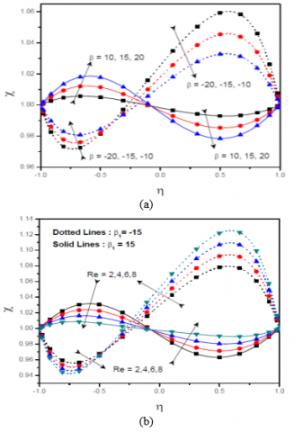
Figure 1. Effect of (a) $\beta_{1}$, (b) Re on $\chi (\eta)$
Figure 1 presents the effect of wall expansion ratio $\beta_{1}$, Reynolds Number Re on the density of the motile microorganisms $\chi (\eta)$ for the wall expansion ratio $\beta_{1}$= -15 and $\beta_{1}$= 15. Figure 1a depicts the variation of $\chi (\eta)$ for different values of $\beta_{1}$. From this figure, it is noticed that, as $\beta_{1}$ increases, the density of the motile microorganisms is also increasing in the first half of the observed region. In other words, near to the lower plate, whether wall contracts or expands, the density of the motile microorganisms is observed to be increasing. Similarly, near to the upper plate, the density of the motile microorganisms is decreasing with an increase in the wall expansion ratio. If $\beta_{1}$ is positive, i.e. the plates are expanding, the density of the motile microorganisms is increased up to a point close to the middle of the channel and exhibits reverse pattern in the upper half of the channel. The reverse trend is observed for the negative values of $\beta_{1}$. The influence of the parameters Re on the density of motile microorganisms is displayed in Figure 1b. If $\beta_{1}$ is positive, the density of the motile microorganisms is growing in the lower half of the channel and lessening in the upper half region of the channel as Re is increasing. Similarly, for $\beta_{1}$ negative, a reverse pattern is observed for increasing values of Re.
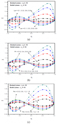
Figure 2. Effect of (a) Le (b) Pr, (c) Pe on $\chi (\eta)$
The effect of Lewis number Le, and bioconvection Peclet Number Pe on the density of the motile microorganisms $\chi$ for the wall expansion ratio $\beta_{1}$= -15 and $\beta_{1}$ = 15 is depicted in Figure 2. Figure 2a displays the variation of the density of motile microorganisms with the Lewis number Le. If the plates are expanding, i.e. for $\beta_{1}$ is positive, the density of the motile microorganisms is increasing in the lower half of the channel and decreasing in the upper half region of the channel as the Lewis number is increasing. As Le is increasing, a decreasing pattern is observed in the lower half region and an increasing pattern in the upper half of the channel is noticed when the plates are contracting. The influence of the parameters Pr and Pe on the density of motile microorganisms is displayed in Figures 2b and 2c. If $\beta_{1}$ is positive, the density of the motile microorganisms is increasing in the lower half of the channel and decreasing in the upper half region of the channel as Re and Pe are increasing. Similarly, for $\beta_{1}$ negative, a reverse pattern is observed for increasing values of Pr and Pe.
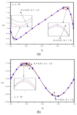
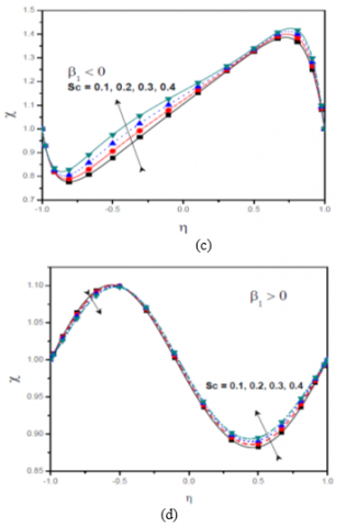
Figure 3. Effect of (a ) S, (b) b1, (c), (d) Sc with b1 on $\chi (\eta)$
Figure 3 represents the variation of the density of motile microorganisms $\chi$ with couple stress parameter S, Schmidt Number Sc. From Figure 3a and Figure 3b, it is interesting to note that the influence of couple stress parameter on the density of motile microorganisms is not significant irrespective of the plates are expanding or contracting. Figure 3c presents the variation of $\chi$ with Sc in $\beta_{1}$ is negative, $\chi$ is diminishing in the lower half of the channel and rising in the upper half region of the channel as Sc is enhanced. The reverse pattern is noticed when the plates are expanding. Figure 3d reveals that the impact of Sc on the density of motile microorganisms is minimal when the plates are expanding while the Schmidt Number has its effect on the fluid when the plates are contrasting.
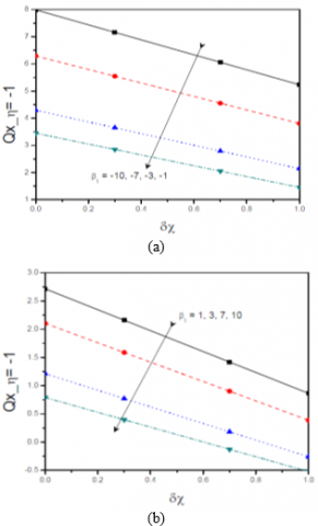
The effects of wall expansion ratio $\beta_{1}$ on the density number of motile microorganisms Qx at the lower and upper plates is presented in Figure 4. When the plates are expanding, the density number of motile microorganisms is increasing at the lower plate as displayed in Figures 4a-4b and the upper plate displayed in Figures 4c-4d. Further, the density number of motile microorganisms is decreasing at the lower plate and increasing at the upper plate when the plates are contracting. Also, Qx is decreasing for increasing values of slip parameter dc at the lower plate and increasing at the upper plate except for $\beta_{1}$> 3 in which it is decreasing.
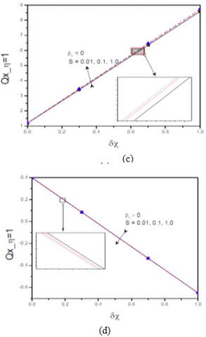
Figure 4. Effect of the parameter $\beta_{1}$ with $\delta \chi$ variation on Qx at $\eta$= -1 (Lower Plate) and $\eta$= 1 (Upper Plate)
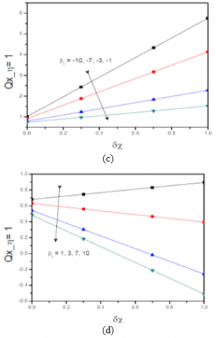
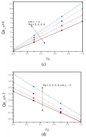
Figure 5. Effect of the parameter Re with dc variation on Qx at $\eta$=-1 (Lower Plate) and $\eta$= 1 (Upper Plate)
The influence of Reynolds Number Re on the density number of motile microorganisms at the lower and upper plates with $\delta \chi$ is portrayed in Figure 5. At the lower plate, as Re increases, Qx is increasing when the plates are expanding/contrasting as shown in Figures 5a-5b. For a given Re as the slip parameter of motile microorganisms increases the Qx is decreasing. Also, at the upper plate, Qx increases with an increase in Re, by showing increasing pattern when $\beta_{1}$ is negative and decreasing in $\beta_{1}$ positive with the slip in motile microorganisms $\delta \chi$ as shown in Figures 5c-5d.
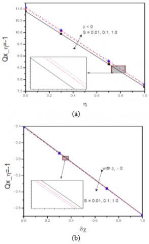
Figure 6. Effect of the parameter S with dc variation on Qx at $\eta$= -1 (Lower Plate) and $\eta$= 1 (Upper Plate)
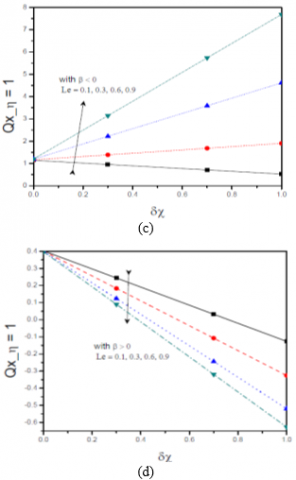
Figure 7. Effect of the parameter Le with dc variation on Qx at $\eta$= -1 (Lower Plate) and $\eta$= 1 (Upper Plate)
The variation of the density number of motile microorganisms at the lower and upper plates with couple stress parameter S is presented in Figure 6 From Figures 6a and 6d it is understood that the impact of couple stress parameter on the density number of the motile microorganisms is insignificant.
The variation of Qx at the lower and upper plates with $\delta \chi$ for different values of Lewis number Le is depicted in Figure 7. It is observed from these figures that Qx is decreasing with $\beta_{1}$ is negative and increasing with $\beta_{1}$ is positive at the lower plate and the similar pattern holds at the upper plate. Also, for a given Le, the Qx decreases as the $\delta \chi$ increase except at the upper plate with $\beta_{1}$ is negative.
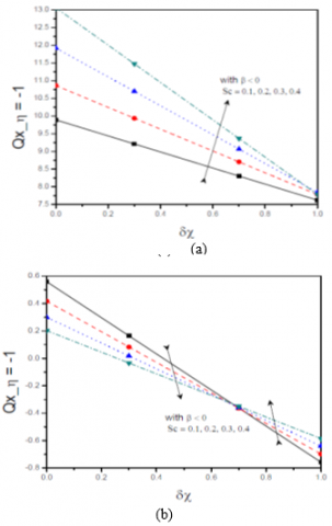
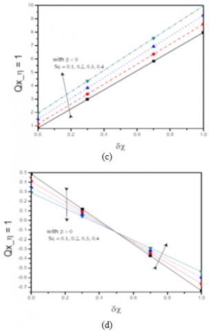
Figure 8. Effect of the parameter Sc with dc variation on Qx at $\eta$=-1 (Lower Plate) and $\eta$=1 (Upper Plate)
The impact of bioconvection Schmidt Number Sc on Qx at the lower and upper plates with $\delta \chi$ is visualized in Figure 8. The Figures 8a and 8b reveals that Qx is increasing as Sc increases when the plates are contrasting at both lower and upper plate and it decreases with up to a critical value and then increases with increase in the value of Sc when the plates are expanding at both the plates, as shown in Figures 8c-8d.
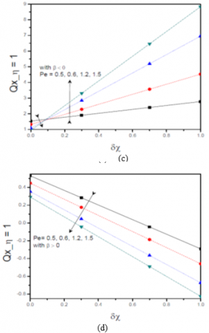
Figure 9. Effect of the parameter Pe with dc variation on Qx at $\eta$=-1 (Lower Plate) and $\eta$=1 (Upper Plate)
The influence of bioconvection Peclet number Pe on the density number of motile microorganisms at the lower and upper plates with $\delta \chi$ is portrayed in Figure (9). At the lower plate, as Pe increases, Qx is increasing when the plates are contracting as shown in Figure (9a) and decreases when plates are expanding as shown in Figure (9b). As Pe is increasing, the density number of the motile microorganisms at the lower plate is also increasing when the plates are contracting. At the upper plate, Qx is decreasing up to a critical value and then increasing in increasing value of Pe for negative $\beta_{1}$. In case of the plates are expanding, the density number of the motile microorganisms is decreasing with an increase in Pe as shown in Figures (9c-9d).
The present analysis deals with the flow of couple stress fluid containing motile microorganisms in a horizontal channel with contracting/expanding porous. The nonlinear ordinary differential equations are linearized using the successive linearization method and solved by implementing the Chebyshev collocation method. The important results are itemized below:
|
A |
A measure of wall permeability |
|
H(t) |
Distance between the plates |
|
bc |
Chemotaxis constant |
|
C |
The concentration of the fluid. |
|
DB |
Mass diffusivity |
|
Dn |
Microorganism diffusivity |
|
f |
Dimensionless stream function |
|
Le |
Lewis Number |
|
S |
couple-stress parameter |
|
Pe |
Bio-convection Peclet number |
|
Pr |
Prandtl number |
|
Qx |
Motile microorganism Density Number |
|
Re |
Permeability Reynolds number |
|
Sc |
Bio-convection Schmidt number |
|
T |
Fluid Temperature |
|
wc |
Maximum cell swimming speed |
|
Greek symbols |
|
|
$\alpha$ |
Thermal Diffusivity |
|
$\beta_{1}$ |
Wall expansion ratio |
|
$\delta \theta, \delta \phi, \delta \chi$ |
Constants |
|
$\eta$ |
Non-dimensional variable |
|
$\theta$ |
Dimensionless temperature |
|
$\vartheta$ |
The density of the motile microorganism. |
|
$\mu$ |
Dynamic Viscosity of the fluid |
|
$v$ |
Magnetic diffusivity/kinetic viscosity |
|
$\rho$ |
Density of the fluid |
|
$\phi$ |
Dimensionless concentration |
|
$\chi$ |
Dimensionless microorganism |
|
Superscripts |
|
|
/ |
Differentiation with respect to $\eta$ |
[1] Stokes, V.K. (1966). Couple stresses in fluids. The Physics of Fluids, 9(9): 1709-1715. https://doi.org/10.1007/978-3-642-82351-0_4
[2] Stokes, V.K. (1984). Theories of Fluids with Microstructures. New York, Springer.
[3] Srivastava, L.M. (1986). Peristaltic transport of a couple-stress fluid. Rheologica Acta, 25(6): 638-641. https://doi.org/10.1007/bf01358172
[4] Pal, D., Rudraiah, N., Devanathan, R. (1988). A couple stress model of blood flow in the microcirculation. Bulletin of mathematical Biology, 50(4): 329-344. https://doi.org/10.1007/BF02459703
[5] Srinivasacharya, D., Srikanth, D. (2012). Steady streaming effect on the flow of a couple stress fluid through a constricted annulus. Arch. Mech., 64(2): 137-152.
[6] Srinivasacharya, D., Madhava Rao, G. (2018). Pulsatile flow of couple stress fluid through a bifurcated artery. Ain Shams Engineering Journal, 9: 883-893. https://doi.org/10.1016/j.asej.2016.04.023
[7] Nabhani, M., El Khilfi, M., Bou-Said, B. (2013). Non-Newtonian couple stress poroelastic squeeze film. Tribol Int, 54: 116-127. https://doi.org/10.1016/j.triboint.2013.03.006
[8] Walicki, E., Walicka, A. (1999). Inertial effect in the squeeze film of couple-stress fluids in biological bearings. Int. J. Appl. Mech. Eng, 4: 363-373.
[9] Islam, S., Zhou, C.Y. (2007). Exact solutions for two-dimensional flows of couple stress fluids. ZAMP, 58: 1035-1048. https://doi.org/10.1007/s00033-007-5075-5
[10] Khan, N.A., Khan, H., Ali, S.A. (2016). Exact solutions for MHD flow of couple stress fluid with heat transfer. Journal of the Egyptian Mathematical Society, 24(1): 125-129. https://doi.org/10.1016/j.joems.2014.10.003
[11] Srinivasacharya, D., Srinivasacharyulu, N., Odelu, O. (2009). Flow and heat transfer of couple stress fluid in a porous channel with expanding and contracting walls. International Communications in heat and Mass Transfer, 36(2): 180-185. https://doi.org/10.1016/j.icheatmasstransfer.2008.10.005
[12] Khan, N.A., Mahmood, A., Ara, A. (2013). Approximate solution of couple stress fluid with expanding or contracting porous channel. Engineering Computations, 30(3): 399-408. https://doi.org/10.1108/02644401311314358
[13] Odelu, O., Naresh Kumar, N. (2014). Hall and ion slip effects on free convection heat and mass transfer of chemically reacting couple stress fluid in a porous expanding or contracting walls with Soret and Dufour effects. Frontiers in Heat and Mass Transfer, 5(1). https://doi.org/10.5098/hmt.5.22
[14] Elkhair, R.E.S.A. (2016). Lie point symmetries for a magneto couple stress fluid in a porous channel with expanding or contracting walls and slip boundary condition. Journal of the Egyptian Mathematical Society, 24(4): 656-665. https://doi.org/10.1016/j.joems.2016.04.001
[15] Pedley, T.J., Hill, N.A., Kessler, J.O. (1988). The growth of bioconvection patterns in a uniform suspension of gyrotactic micro-organisms. Journal of Fluid Mechanics, 195: 223-237. https://doi.org/10.1017/S0022112088002393
[16] Childress, S., Levandowsky, M., Spiegel, E.A. (1975). Pattern formation in a suspension of swimming microorganisms: equations and stability theory. Journal of Fluid Mechanics, 69(3): 591-613. https://doi.org/10.1017/S0022112075001577
[17] Shaw, S., Sibanda, P., Sutradhar, A., Murthy, P.V.S.N. (2014). Magnetohydrodynamics and soret effects on bioconvection in a porous medium saturated with a nanofluid containing gyrotactic microorganisms. Journal of Heat Transfer, 136(5): 052601. https://doi.org/10.1115/1.4026039
[18] Xu, H., Pop, I. (2014). Mixed convection flow of a nanofluid over a stretching surface with uniform free stream in the presence of both nanoparticles and gyrotactic microorganisms. International Journal of Heat and Mass Transfer, 75: 610-623. https://doi.org/10.1016/j.ijheatmasstransfer.2014.03.086
[19] Raees, A., Xu, H., Liao, S.J. (2015). Unsteady mixed nano-bioconvection flow in a horizontal channel with its upper plate expanding or contracting. International Journal of Heat and Mass Transfer, 86: 174-182. https://doi.org/10.1016/j.ijheatmasstransfer.2015.03.003
[20] Raju, C.S., Sandeep, N. (2016). Dual solutions for unsteady heat and mass transfer in bio-convection flow towards a rotating cone/plate in a rotating fluid. In International Journal of Engineering Research in Africa, 20: 161-176. https://doi.org/10.4028/www.scientific.net/JERA.20.161
[21] Makinde, O.D., Animasaun, I.L. (2016). Bioconvection in MHD nanofluid flow with nonlinear thermal radiation and quartic autocatalysis chemical reaction past an upper surface of a paraboloid of revolution. International Journal of Thermal Sciences, 109: 159-171. https://doi.org/10.1016/j.ijthermalsci.2016.06.003
[22] Mosayebidorcheh, S., Tahavori, M.A., Mosayebidorcheh, T., Ganji, D.D. (2017). Analysis of nano-bioconvection flow containing both nanoparticles and gyrotactic microorganisms in a horizontal channel using modified least square method (MLSM). Journal of Molecular Liquids, 227: 356-365. https://doi.org/10.1016/j.molliq.2016.12.039
[23] Zhao, Q., Xu, H., Tao, L. (2017). Unsteady bioconvection squeezing flow in a horizontal channel with chemical reaction and magnetic field effects. Mathematical Problems in Engineering. https://doi.org/10.1155/2017/2541413
[24] Bin-Mohsin, B., Ahmed, N., Khan, U., Mohyud-Din, S. T. (2017). A bioconvection model for a squeezing flow of nanofluid between parallel plates in the presence of gyrotactic microorganisms. The European Physical Journal Plus, 132(4): 187. https://doi.org/10.1140/epjp/i2017-11454-4
[25] Khan, S.U., Waqas, H., Bhatti, M.M., Imran, M. (2020). Bioconvection in the rheology of magnetized couple stress nanofluid featuring activation energy and Wu’s slip. Journal of Non-Equilibrium Thermodynamics, 45(1): 81-95. https://doi.org/10.1515/jnet-2019-0049
[26] Makukula, Z.G., Sibanda, P., Motsa, S.S. (2010). A novel numerical technique for two-dimensional laminar flow between two moving porous walls. Mathematical Problems in Engineering. https://doi.org/10.1155/2010/528956
[27] Canuto, C., Hussaini, M.Y., Quarteroni, A., Zang, T.A. (2006). Spectral Methods. Springer.
[28] Trefethen, L.N. (2000). Spectral Methods in MATLAB. Oxford University, Oxford, England. https://doi.org/10.1137/1.9780898719598