OPEN ACCESS
Fluid dynamic systems are usually optimised through the equation of conservation of energy according to the first law of thermodynamics. In the aeronautic sector, many authors are claiming the insufficiency of this approach and are developing studies and models with the aim of coupling the analyses according to the first and the second law of thermodynamics. Second law analysis of internal fluid dynamics has not been studied with the same attention. Just heat exchangers and heat dissipation by electronic circuits are mostly considered. This paper focuses on the analysis of general internal fluid flow problem and recognizes initially it according to the first law of thermodynamics. The energy equation for a control volume is given in integral form along with a discussion on the concepts of total energy, heat and work. The dissipative terms, which need to be minimised to increase the system efficiency, are deeply analysed leading to a new dimensionless formulation of the equation of conservation of energy. It is based on Bejan number, according to the formulation by Bhattacharjee and Grosshandler. This formulation has been directly connected to second law analysis concerning both entropy generation and exergy dissipation making a step toward a future unification of the two alternative formulations of Bejan number which have been historically developed. The ambition of this research is far from providing a definitive solution. Otherwise, it aims to both raise problems and stimulate a discussion. Bejan number has been actually used in the definition of diffusive phenomena, such as convection and diffusion through porous media. Is it reasonable to enlarge its domain to the much larger domain of general fluid dynamics? If this extension will be evaluated possible, what are the potential implications for the future of scientific research? Can be the ambiguity between Hagen number and Bejan number be resolved? Can be the ambiguity between the diffusive definition and the entropy generation definition of Bejan number be solved? Can it be possible to state the equivalence between the two alternative formulations? Is it possible to define fluid dynamic and diffusive problems according to a unified vision in the domain of thermodynamics? What are the implications concerning analysis and optimisation of fluid dynamics phenomena by new equations that couples first and the second law of thermodynamics? Could it have the role of producing an effective unification of a larger multidisciplinary domain?
fluid dynamics, conservation laws, Bejan number, Bejan energy, entropy generation, Hagen number
The analysis of general fluid flows inside an arbitrary control volume, which has been performed in this paper, connects to the intuition, which has been presented by Liversage [1] in the Bachelor final year project. He studied the drag reduction effects by a sharkskin surface with triangular profiles. He made some considerations on the drag force in fluid dynamics:
$D=\frac{1}{2} C_{D} A_{f} \rho u^{2}$ (1)
After taking into account the analysis of fluid dynamic dissipation in pipes by Medina et al. [2] managed to rewrite the drag expression in equation (1). If the drag force is expressed by the identity D=AwΔp and both sides of equation (1) are multiplied by μ2/(ρ l2), he obtained equation (2), which is reported below.
$D=\Delta p_{D} A_{w}=\frac{1}{2} C_{D} A_{f} \frac{\mu^{2}}{\rho l^{2}} \frac{\rho^{2} u^{2} l^{2}}{\mu^{2}}=\frac{1}{2} C_{D} A_{f} \frac{\mu v}{l^{2}} \operatorname{Re}^{2}$ (2)
Equation (2) can be expressed in the following form.
$C_{D}=2 \frac{A_{w}}{A_{f}} \frac{\Delta p_{D} \rho l^{2}}{\mu^{2}} \frac{1}{\operatorname{Re}^{2}}=2 \frac{A_{w}}{A_{f}} \frac{\Delta p_{D} l^{2}}{\mu \nu} \frac{1}{\operatorname{Re}^{2}}$ (3)
Liversage and Trancossi [4] have observed that
$B e=\frac{\Delta p \cdot l^{2}}{\mu v}$ (4)
is identical to Bejan number as defined by Bhattacharjee et al. [3] and have rewritten equation (3) consequently.
$C_{D}=2 \cdot \frac{A_{w}}{A_{f}} \cdot \frac{B e}{\operatorname{Re}^{2}}$ (5)
where CD is the drag coefficient, Aw is the wet area, and Af is the front area.
A better analysis of the nature of friction, which has evidenced that fluid dynamic drag, is composed of two major components, one relates to the shear stress with the walls, and the other relates to the viscosity. A detailed analysis on fluid dynamic dissipations models has been performed with particular attention to Betz [5], Maskell [6], Ashforth-Frost et al. [7], Kin et al. [8], Drela [9], Sato [10] and Bhattacharyya et al. [11]. Two different pressure jumps have been identified Δpτ, which relates to shear stress, and Δpν, which relates to viscous phenomena in the boundary layer. The equation of CD has been rewritten in the following form:
$C_{D}=2 \cdot \frac{A_{w}}{A_{f}} \cdot \frac{B e_{\tau}+B e_{v}}{\operatorname{Re}^{2}}$ (6)
The activity by Liversage and Trancossi which has hypothesised the relation of Bejan number and fluid dynamic drag let open a series of problems which have high scientific value in the study of fluid dynamics and convective exchange problems.
Does the connection between Bejan number and fluid dynamic drag allow thinking to more extensive involvement of Bejan number into the representation of fluid dynamic phenomena?
Considering the similar formulations of Bejan and Hagen numbers [12-14], what is the correct dimensionless number to represent fluid dynamic dissipations?
Two different dimensionless magnitudes have been independently defined as Bejan number. Bejan and Sciubba [15] have envisaged the diffusive formulation, Bhattacharjee et al. have explained it in terms of the momentum diffusivity of the fluid (kinematic viscosity ν), Petrescu [16] has described it in terms of thermal diffusivity α of the fluid, Awad [17] has formulated it in terms of mass diffusivity D of the fluid in porous systems. This formulation has been generalised by Awad diffusive Bejan Number, which has been extended by Awad [18], who have demonstrated that the diffusive formulations reduce to the same quantity if Reynolds analogy being valid (Pr = Sc = 1). Sciubba [19] has defined the thermodynamic formulation of Bejan number as the ratio between entropy generation by convective heat transfer and total entropy generation. Is it possible to express the diffusive Bejan number concerning second law of thermodynamics? Is it possible to resolve the dualism between the two formulations? Is it possible to define particular conditions under which the two definitions can be coincident?
Is it possible to use the Bejan number to create an adequate description of fluid dynamic phenomena according to the second law of thermodynamics to enlarge the possibilities of optimisation of a fluid dynamic system through the options which are offered by exergy of entropy generation techniques?
This paper aims to start a discussion on the above-opened problems in modern thermodynamics. It will attempt to give an even still partial and problematic answer to the above questions in the case of a very general fluid dynamic system in which a flow is moving on an arbitrary path which develops inside an arbitrary domain with inlets and outlets. It will also analyse if further problems, which may arise.
The fluid flow in an arbitrary domain is a fundamental and well-referenced problem that will be considered in the attempt of approaching the above questions. It is an internal fluid dynamic problem, which can be described by the three conservation laws. In particular, the flow of a generic flow into an arbitrarily shaped pipe has been considered (Figure 1).
It will be analysed in the case of both an incompressible fluid and a compressible fluid with arbitrary inlet conditions and hydrostatic jump. Arbitrarily, it is possible to consider pumps that transfer a certain amount of work to the fluid, turbines that receive work from the fluid, and an arbitrary amount of heated and cooled surfaces.
A general schematization of the considered problem with the related domain is presented in Figure 1.
Figure 1. Schematization of the generic considered domain
The steady state of any fluid system [20-21] with inlets and outlets can be described by equation of conservation of mass and equation of conservation of energy for the control volume with inlets and outlets of mass, energy, work together with internal dissipations. Subscripts 'i' and 'e' indicate inflows and outflows of mass. The case of an incompressible fluid flow is considered (r=const).
2.1 Conservation of mass
The law of conservation of mass [22] becomes:
$\dot{m}=\dot{m}_{i}=\rho A_{i} u_{i}=\dot{m}_{e}=\rho A_{e} u_{e}=$const (7)
where subscripts 'i' and 'e' indicate energy inflows and outflows respectively. The equation can be expressed in a dimensionless form by multiplying both terms by L/(μAw) and becomes
$\frac{A_{i}}{A_{w}} \frac{L \rho u_{i}}{\mu}=\frac{A_{e}}{A_{w}} \frac{L \rho u_{e}}{\mu}$ (8)
2.3 Conservation of momentum
The third and more complex equation, which describes a fluid flow, relates to the law of conservation of momentums. Linear momentum equation for fluids can be developed by starting from Newton's 2nd Law. The sum of all forces applied on the control volume equals the time rate of change of the momentum.
$\sum_{i} \mathbf{F}_{i}=\frac{d}{d t}(m \cdot \mathbf{u})$ (9)
It is evident that equation (9) can be easily applied in the domain of particle mechanics. Otherwise in fluid mechanics [23] the integral application to a control volume (and not to individual particles) require computing the momentum inside the control volume, and the momentum passing through the surface. It can be consequently being expressed in the following general formulation, which has been obtained by Reynolds Transport Theorem.
$\sum_{i} \mathbf{F}_{i}=\frac{\partial}{\partial t} \int_{C V} \rho \mathbf{u} d u+\int_{C S} \mathbf{u} \rho \mathbf{u} \cdot \mathbf{n} d A$ (10)
where u is the velocity vector, n is the outward normal unit vector, and ΣF is the sum of all forces (body and surface forces), which are applied to the control volume.
The law of conservation of linear momentum states that the sum of all forces applied on the control volume is equal to the sum of the rate of change of momentum inside the control volume and the net flux of momentum through the control surface.
For steady flow, the rate of change of momentum inside the control volume vanishes. The sign of the force and velocity vectors (F and V) depends on the assigned coordinate system. The sign on the quantity u·n depends on the orientation of both velocity and the control surface. The unit normal vector n is usually assumed positive when it points out of the control surface.
In the case of the flow of a fluid in an arbitrary complex piping system, the conservation of momentum can be simplified for steady state conditions. In this case, it can be assumed that the control volume presents simple and localized inlets and outlets and piping, whatever complex they are connects inlets and outlets, the momentum equation becomes
$\Sigma F=\sum_{e}(\rho A V \mathbf{V})_{e}-\sum_{i}(\rho A V \mathbf{V})_{i}$ (11)
If we consider the conservation of mass law, the following formulation can be achieved:
dm/dt = ρAV,
and the momentum equation simplifies to
$\sum_{i} \mathbf{F}_{i}=\sum_{e} \frac{d m_{e}}{d t} \mathbf{u}_{e}-\sum_{i} \frac{d m_{i}}{d t} \mathbf{u}_{i}$ (12)
where e represents outflow and i inflow. It must be remarked that any force that exercise its action on the world outside the domain must be computed, including weight reactions and the resultants of induced shear stresses.
Equation 34 can be expressed in an explicit way as follows:
$\sum_{i} \mathbf{F}_{i}=\sum_{e} \rho A_{e} u_{e} \mathbf{u}_{e}-\sum_{i} \rho A_{i} u_{i} \mathbf{u}_{i}$ (13)
By considering the domain in Figure 1, the useful representation of the domain for the specific calculation is represented below in Figure 2.
Figure 2. Domain and characteristic vectors for the assessment of equation of conservation
In the particular case, which has considered and is presented in Figure 1 and 2, the equations of conservation of momentums can be expressed as:
$\left\{\begin{array}{l}{p_{i} A_{i}-p_{e} A_{e}+R_{x}=u_{i} \rho\left(-u_{i}\right) A_{i}+u_{e} \rho\left(u_{e}\right) A_{e}} \\ {-W+R_{z}=0}\end{array}\right.$ (14)
and can be expressed as follows
$\left\{\begin{array}{l}{p_{i} A_{i}-p_{e} A_{e}+R_{x}=-\rho u_{i}^{2} A_{i}+\rho u_{e}^{2} A_{e}} \\ {-V \rho g+R_{z}=0}\end{array}\right.$ (15)
By multiplying the two equations by L2/(Airν2), it results:
$\left\{\begin{array}{l}{\frac{p_{i} L^{2} A_{i}}{\rho v^{2} A_{w}}-\frac{p_{e} L^{2} A_{e}}{\rho v^{2} A_{w}}+\frac{L^{2} R_{x}}{\rho v^{2} A_{w}}=-\frac{\rho u_{i}^{2} L^{2} A_{i}}{\rho v^{2} A_{w}}+\frac{\rho u_{e}^{2} L^{2} A_{e}}{\rho v^{2} A_{w}}} \\ {-\frac{V \rho g L^{2}}{A_{w} \rho v^{2}}+\frac{L^{2} R_{z}}{\rho v^{2} A_{w}}=0}\end{array}\right.$ (16)
in which Rx and Rz are the reactions over x and z-axis. It can also be remarked that all the terms have the same dimensions of Bejan number.
2.2 Conservation of energy
The first law of thermodynamics states that energy can neither be created nor destroyed, but only change forms. It can be represented by a set of integral terms, one for the control volume, and one for the control surface, that consider that new energy can be added or subtracted from the system through heat and work. The integral form of the equation of conservation of energy [24-25] in fluids is expressed below.
$\underbrace{\dot{m}\frac{u_{i}^{2}}{2}+\dot{m}g{{z}_{i}}+\frac{{\dot{m}}}{\rho }{{p}_{i}}}_{ENERGY\text{ }IN}+\underbrace{{{{\dot{W}}}_{in}}}_{\begin{smallmatrix} WORK \\ IN \end{smallmatrix}}+\underbrace{{{{\dot{Q}}}_{in}}}_{\begin{smallmatrix} HEAT \\ IN \end{smallmatrix}}==\underbrace{\dot{m}\frac{u_{e}^{2}}{2}+\dot{m}g{{z}_{e}}+\frac{{\dot{m}}}{\rho }{{p}_{e}}}_{ENERGY\text{ }OUT}+\underbrace{{{{\dot{W}}}_{out}}}_{\begin{smallmatrix} WORK \\ OUT \end{smallmatrix}}+\underbrace{{{{\dot{Q}}}_{out}}}_{\begin{smallmatrix} HEAT \\ OUT \end{smallmatrix}}+\underbrace{\frac{{\dot{m}}}{\rho }\Delta {{p}_{L}}}_{LOSSES}$ (17)
Equation (17) is the general equation for the specific fluid flow with mass inflows and outflows and energy and work inlets and outlets. To express a dimensionless formulation of equation (17) after dividing by the mass flow $\dot{m}$ both sides of the equation.
$\frac{u_{i}^{2}}{2}+g z_{i}+\frac{p_{i}}{\rho}+\frac{\dot{W}_{i n}}{\dot{m}}+\frac{\dot{Q}_{i n}}{\dot{m}}=\frac{u_{e}^{2}}{2}+g z_{e}+\frac{p_{e}}{\rho}+\frac{\dot{W}_{o u t}}{\dot{m}}+\frac{\dot{Q}_{o u t}}{\dot{m}}+\frac{\Delta p_{L}}{\rho}$
It is possible to multiply both terms of the equation by the same dimensionless quantity L2/n2.
$\frac{L^{2} u_{i}^{2}}{2 v^{2}}+\frac{L^{2} g z_{i}}{v^{2}}+\frac{L^{2} p_{i}}{\rho v^{2}}+\frac{L^{2}}{v^{2}} \frac{\dot{W}_{i n}}{\dot{m}}+\frac{L^{2}}{v^{2}} \frac{\dot{Q}_{i n}}{\dot{m}}=$=\frac{L^{2} u_{e}^{2}}{2 \rho v^{2}}+\frac{L^{2} g z_{e}}{v^{2}}+\frac{L^{2} p_{e}}{\rho v^{2}}+\frac{L^{2}}{v^{2}} \frac{\dot{W}_{o u t}}{\dot{m}}+\frac{L^{2}}{v^{2}} \frac{\dot{Q}_{o u t}}{\dot{m}}+\frac{L^{2} \Delta p_{L}}{\rho v^{2}}$ (18)
Equation (18) shows that the dimensionless dissipative term has the same dimensions of Bejan number.
The last term of equation (18) allows verifying that the hypothesis by Liversage and Trancossi is coherent with the energy conservation law in fluid dynamics, even if a more in-depth analysis on this dissipative term is necessary.
2.4 General dimensionless expression of conservation laws
It can be possible to express a general form of the conservation laws by the following system of equations.
$\frac{A_{i}}{A_{w}} \frac{L \rho u_{i}}{\mu}=\frac{A_{e}}{A_{w}} \frac{L \rho u_{e}}{\mu}$ (19)
$\frac{L^{2} p_{i}}{\rho v^{2}} \frac{A_{i}}{A_{w}}-\frac{L^{2} p_{e}}{\rho v^{2}} \frac{A_{e}}{A_{w}}+\frac{L^{2} R_{x}}{\rho v^{2} A_{w}}=-\frac{L^{2} u_{i}^{2}}{v^{2}} \frac{A_{i}}{A_{w}}+\frac{L^{2} u_{e}^{2}}{v^{2}} \frac{A_{e}}{A_{w}}$ (20)
$-\frac{L^{2} V \rho g}{A_{w} \rho v^{2}}+\frac{L^{2} R_{z}}{\rho v^{2} A_{w}}=0$ (21)
$\frac{L^{2} u_{i}^{2}}{2 v^{2}}+\frac{L^{2} g z_{i}}{v^{2}}+\frac{L^{2} p_{i}}{\rho v^{2}}+\frac{L^{2}}{v^{2}} \frac{\dot{W}_{i n}}{\dot{m}}+\frac{L^{2}}{v^{2}} \frac{\dot{Q}_{i n}}{\dot{m}}==\frac{L^{2} u_{e}^{2}}{2 v^{2}}+\frac{L^{2} g z_{e}}{v^{2}}+\frac{L^{2} p_{e}}{\rho v^{2}}+\frac{L^{2}}{v^{2}} \frac{\dot{W}_{o u t}}{\dot{m}}+\frac{L^{2}}{v^{2}} \frac{\dot{Q}_{o u t}}{\dot{m}}+\frac{L^{2} \Delta p_{L}}{\rho v^{2}}$ (22)
As noticed above, the terms of the four equations have the same dimensions of Bejan number, even if they differ from Bejan number, because of they a function of a pressure jump, but the local pressure defines them in a well-defined point of the system.
While Bejan number depends on the pressure jump between two different states, the dimensionless terms in those equations have identical dimensions but slightly different meaning for Bejan number. These terms do not include the pressure jump between two points in a system, but they contain the dimensionless pressure value in a point of the system. As we see from equation 18 all the terms are equal to a dimensionless power (energy divided by time).
It is consequently necessary to differentiate them from the Bejan number, because of the different meaning. These dimensionless magnitudes can be defined as Bejan dimensionless energy. Therefore the traditional formulation of Bejan number is equal to the Bejan number and they are identified by the Greek letter x.
$\xi_{j}=\frac{L^{2} p_{j}}{\rho v^{2}}$
These considerations allow writing that Bejan number is the difference of two Bejan dimensionless energies with the same nature:
$\mathrm{Be}=\frac{L^{2} p_{j}}{\rho v^{2}}-\frac{L^{2} p_{h}}{\rho v^{2}}=\xi_{j}-\xi_{h}$
The following substitution can be done
$\operatorname{Re}_{L, j}=\frac{L \rho u_{j}}{\mu}=\frac{L u_{j}}{v}$ (23)
ReL,j is the Reynolds number related for the entire length of the pipe for the generic j velocity condition.
The quadratic term can require further considerations
$\operatorname{Re}_{L, j}^{2}=\frac{L^{2} u_{j}^{2}}{v^{2}}=2 \frac{L^{2}}{\rho v^{2}}\left(\frac{\rho}{2} u_{j}^{2}\right)=2 \frac{L^{2}}{\rho v^{2}} p_{k, j}=2 \frac{L^{2}}{v \mu} p_{k, j}$,
which is the dimensionless kinetic energy, where pk,j is the dynamic pressure exerted by a fluid flowing at velocity uj.
$\operatorname{Re}_{L, j}=\sqrt{\xi_{k, j}}$ (24)
$\frac{L^{2}\left(\rho g z_{j}\right)}{\rho v^{2}}=\frac{L^{2} p_{z, j}}{\rho v^{2}}=\frac{L^{2} p_{z, j}}{v \mu}=\xi_{z, j}$ (25)
is dimensionless hydrostatic pressure, where pz,j is the hydrostatic pressure exerted by a fluid with a hydrostatic height zj.
$\frac{L^{2} p_{j}}{\rho v^{2}}=\frac{L^{2} p_{j}}{v \mu}=\xi_{p, j}$ (26)
is dimensionless pressure where pj is the pressure of the fluid in the generic position j.
$\frac{L^{2} R_{x}}{\rho v^{2} A_{w}}=\frac{L^{2}}{\rho v^{2}} \frac{R_{x}}{A_{w}}=\frac{L^{2} p_{R_{x}}}{v \mu}=\xi_{R x}$ (27)
is a dimensionless horizontal reaction, where $p_{R_{x}}$ is the ratio of the reaction Rx and the wet area Aw;
$\frac{L^{2} R_{z}}{\rho v^{2} A_{w}}=\frac{L^{2}}{\rho v^{2}} \frac{R_{z}}{A_{w}}=\frac{L^{2} p_{R_{z}}}{v \mu}=\xi_{R z}$ (28)
is the dimensionless vertical reaction, where $P_{R_{z}}$ is the ratio of the reaction Rz and the wet area Aw;
$\frac{L^{2} V \rho g}{A_{w} \rho v^{2}}=\frac{L^{2}}{v \mu} \frac{m g}{A_{w}}=\frac{L^{2} p_{m}}{v \mu}=\xi_{m}$ (29)
is a dimensionless weight of fluid in the pipe where pm is the ratio of the weight of fluid inside the tube and the wet area Aw;
$\frac{L^{2}}{v^{2}} \frac{\dot{W}_{j}}{\dot{m}}=W_{j}^{*}$ (30)
is dimensionless mechanical power;
$\frac{L^{2}}{v^{2}} \frac{\dot{Q}_{j}}{\dot{m}}=Q_{j}^{*}$ (31)
is dimensionless heat power;
$\frac{L^{2} \Delta p_{L}}{\rho v^{2}}=\frac{L^{2} \Delta p_{L}}{v \mu}=B e_{L}$ (32)
is dissipative losses.
$\frac{A_{j}}{A_{w}}=A_{j}^{*}$ (33)
is the dimensionless area of the generic section j of the domain.
Consequently, the dimensionless equations become:
$A_{i}^{*} \sqrt{\xi_{k, i}}=A_{e}^{*} \sqrt{\xi_{k, e}}$ (34)
or
$A_{i}^{*} \operatorname{Re}_{L, i}=A_{e}^{*} \operatorname{Re}_{L, e}$ (34’)
$\xi_{p, i} A_{i}^{*}-\xi_{p, \mathrm{e}} A_{e}^{*}+\xi_{R x}=-\operatorname{Re}_{L, i}^{2} A_{i}^{*}+\operatorname{Re}_{L, e}^{2} A_{e}^{*}$ (35)
or
$\xi_{p, i} A_{i}^{*}-\xi_{p, \mathrm{e}} A_{e}^{*}+\xi_{R x}=-\xi_{k, i} A_{i}^{*}+\xi_{k, e} A_{e}^{*}$ (35’)
$-\xi_{m}+\xi_{R z}=0$ (36)
$\operatorname{Re}_{L, i}^{2}+\xi_{z, i}+\xi_{p, i}+\dot{W}_{i n}^{*}+\dot{Q}_{i n}^{*}==\operatorname{Re}_{L, \mathrm{e}}^{2}+\xi_{z, e}+\xi_{p, e}+\dot{W}_{o u t}^{*}+\dot{Q}_{o u t}^{*}+\mathrm{Be}_{L}$ (37)
or
$\xi_{k, i}+\xi_{z, i}+\xi_{p, i}+\dot{W}_{i n}^{*}+\dot{Q}_{i n}^{*}==\xi_{k, \mathrm{e}}+\xi_{z, e}+\xi_{p, e}+\dot{W}_{o u t}^{*}+\dot{Q}_{o u t}^{*}+\mathrm{Be}_{L}$ (37’)
It is evident that equations (32’) can be expressed in two competitive formulations that can be used for solving different problems. The first one focuses on the initial and final state conditions, which are evidenced:
$\xi_{t o t, i}+\dot{W}_{i n}^{*}+\dot{Q}_{i n}^{*}=\xi_{t o t, \mathrm{e}}+\dot{W}_{o u t}^{*}+\dot{Q}_{o u t}^{*}+\mathrm{Be}_{L}$ (37’’)
where
$\xi_{t o t, j}=\xi_{k, j}+\xi_{z, j}+\xi_{p, j}$.
The second one focuses on the differences between inlet and outlet conditions and becomes:
$\left(\xi_{k, i}-\xi_{k, \mathrm{e}}\right)+\left(\xi_{z, i}-\xi_{z, e}\right)+\left(\xi_{p, i}-\xi_{p, e}\right)+\dot{W}_{i n}^{*}+\dot{Q}_{i n}^{*}==\dot{W}_{o u t}^{*}+\dot{Q}_{o u t}^{*}+\mathrm{Be}_{L}$
that corresponds to
$\mathrm{Be}_{k}+\mathrm{Be}_{z}+\mathrm{Be}_{p}+\dot{W}_{i n}^{*}+\dot{Q}_{i n}^{*}=\dot{W}_{o u t}^{*}+\dot{Q}_{o u t}^{*}+\mathrm{Be}_{L}$. (37’’’)
Both formulations lead to a more compact formulation, that focuses into a unified vision of the inlet and the outlet energy states and it is reported in equation
$B e_{t o t}=\Delta \dot{W}^{*}+\Delta \dot{Q}^{*}+\mathrm{Be}_{L}$ (38)
where
$\mathrm{Be}_{t o t}=\mathrm{Be}_{k}+\mathrm{Be}_{z}+\mathrm{Be}_{p}=\xi_{t o t, i}+\xi_{t o t, \mathrm{e}}$.
2.5 Consideration on Bejan number and the defined Bejan dimensionless energy
The dimensionless expression of the conservation equations (19) to (22) has allowed defining a new local dimensionless magnitude, which is derived from the traditional definition of Bejan number by Bhattacharjee et al. and generalised by Awaz. It appears as a local formulation of Bejan number, which characterises inlets and outlets of the domain or subdomain and applies in any arbitrary point of a fluid dynamic system. If we consider the diffusive definition of Bejan number as expressed in equation (4), it is evident that it can be expressed as
$B e=\frac{\Delta p \cdot l^{2}}{\mu v}=\frac{\left(p_{1}-p_{2}\right) \cdot l^{2}}{\mu v}$ (39)
where p1 and p2are the pressure conditions in two arbitrary points 1 and 2. Consequently, it is possible to hypothesise that the traditionally defined Bejan number can be expressed as the difference of two local dimensionless energies.
In this case, if dimensionless energy (which has the dimension of the Bejan number) has been indicated with the Greek letter x
$\xi=\frac{p \cdot l^{2}}{\mu v}$
and equation (39) becomes
$B e=\frac{\Delta p \cdot l^{2}}{\mu v}=\frac{\left(p_{1}-p_{2}\right) \cdot l^{2}}{\mu v}=\xi_{1}-\xi_{2}$
It is possible to describe the state of an arbitrary point of the system by a dimensionless number that accounts the characteristic properties of the fluid in the specified position, which are kinetic energy, potential energy and pressure energy if considered in the first two cases according to their pressure equivalences:
This local dimensionless number is defined below.
$\xi=\frac{L^{2}}{v^{2}}\left(\frac{1}{2} \rho u^{2}+\rho g z+p\right)=\frac{L^{2}}{\rho v^{2}}\left(\frac{1}{2} \rho u^{2}+\rho g z+p\right)$ (42)
From equation (42) it is possible to express Bei-e as
$\mathrm{Be}_{i-e}=\left(\xi_{k, i}+\xi_{z, i}+\xi_{p, i}\right)-\left(\xi_{k, e}+\xi_{z, e}+\xi_{p, e}\right)$ (43)
Equations (28), (29) and (43) open a series of questions about the definition of Bejan number. In particular, Bejan number presents the characteristics of being considered a difference of two dimensionless energy states that defines uniquely the energy in a point of a system, whatever is the sum of the energy components that constitute it.
Dimensionless energy expressed by equation (30) could be named as Bejan energy because it represents the dimensionless energy x of one of the points between which Bejan number is calculated.
Bejan number is a potentially constitutive dimensionless magnitude of fluid dynamics and represents the dimensionless difference between two energy states inside the system in which a fluid flows. It is also evident that the conservation law as formulated by using Bejan number could produce significant benefits in the numerical calculation because they contain significant simplifications of the number of computed magnitudes and could allow a major simplification of the equation to be computed and a possible reduction of computational errors in numerical computations.
Recently Herwig and Schmandt [26] have studied dissipative and friction phenomena in fluid dynamics. Any real process generates losses of mechanical energy that increases the internal energy. This energy conversion process maintains the total energy of the system and deals strictly with energy availability and usefulness. Consequently, it belongs strictly to the second law of thermodynamics. It can be expressed in both entropy generation terms and exergetic terms as a loss of exergy or available work, corresponding to degradation of available energy in the flow field.
3.1 Nature of fluid dynamic losses
Fluid dynamic losses can be expressed in different ways depending on their nature.
Scientific literature reports two different formulations. One is the Colebrook, and White friction factor [27-29] has been formulated in equation (44):
$\frac{d p}{d x}=-\frac{f}{D} \frac{\rho}{2} u_{a v}^{2} \rightarrow \Delta P \simeq f \frac{L}{D} \frac{\rho}{2} u_{a v}^{2}$ (44)
In equation 39, the friction coefficient f is the Fanning friction factor, which is the ratio between the local shear stress and the local flow kinetic energy density. Equation (39) is a function of wall friction coefficient and represents the resultant of wall shear stresses.
Internal flow losses can also be expressed in terms of head loss coefficient K [30-32] according to the well-known formulation below:
$\Delta P=K \frac{\rho}{2} u_{a v}^{2}$. (45)
Friction losses are expressed in terms of drag force [33-36], which is a formulation which accounts the head losses. It is a function of drag coefficient according to equation (46):
$F_{D}=C_{D} \frac{\rho}{2} u_{\infty}^{2} A_{f}$. (46)
The different formulations of the fluid flow losses which have been defined present different nature and can be observed that they have distinct natures and different values.
It must be noticed that dissipative, and skin friction formulations of drag do not bring to the same results, because they have very different natures as Drela [37] has observed.
Skin friction model focuses on what happens on the surface and can be defined by the following equation.
$D_{f}=\iint\left[\tau_{x y}\right]_{y=0} d x d z=\iint \rho_{e} U_{\infty}^{3} C_{f} d x d z$ (47)
On the other side, dissipation terms consider all the losses in the boundary layer along its complete development, including also what happens in the boundary layer and after detachment.
$\Phi=\iint\left[\int_{0}^{\delta} \tau_{x y} \frac{\partial u}{\partial y} d y\right] d x d z=\iint \rho_{e} U_{\infty}^{3} C_{D} d x d z$ (48)
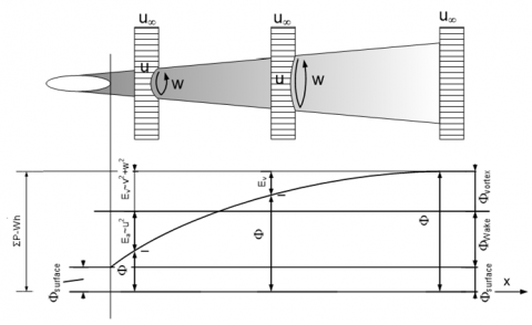
The meaning of the two terms can be explained at domain level by figure 3 in a case of external fluid dynamics and by Figure 4 in the case of internal fluid dynamics.
Figure 3. Dissipative terms and their graphical representation in external fluid dynamics
Figure 4. Dissipative terms and their graphical representation in internal fluid dynamics
In this paper, we account the losses according to the dissipative model, because they give an exhaustive answer to the problem of the determination of losses.
3.2 Dissipations and the second law of thermodynamics
It must also be remarked that the fluid dynamic dissipations can be expressed concerning the second law of thermodynamics. $\dot{S}$ The processes can be analyzed [38-41] in terms of both entropy generation and exergy destruction rate:
$\dot{E} x_{L}=T_{0} \dot{S}_{g e n}$ (49)
The dissipated mechanical power is equal to
$\dot{E}_{L}=F_{D} \cdot u_{\infty}=\Delta P \cdot A \cdot u_{\infty}=T \cdot \dot{S}_{g e n, f}$, (50)
The case of an internal and an external fluid dynamic problem are reported below.
In the case of external flows the dissipated mechanical power is
$\dot{E}_{L}=C_{D} \frac{\rho}{2} u_{\infty}^{3} A_{f}=T \dot{S}_{g e n, f}$ (51)
from which it can be obtained
$C_{D}=\frac{2 T}{A_{f} \rho u_{\infty}^{3}} \dot{S}_{g e n, f}$ (52)
Equation (52) can be substituted into (46) obtaining the entropic expression of friction force.
$F_{D}=C_{D} \frac{\rho}{2} u_{\infty}^{2} A_{f}=\frac{T}{u_{\infty}} \dot{S}_{g e n, f}$ (53)
It is possible to express the dissipated mechanical power by equation (54):
$p_{L}=K A_{w} \frac{\rho}{2} u_{i}^{3}=T \cdot \dot{S}_{g e n, f}$ (54)
that allows obtaining
$K=\frac{2 T}{A_{w} \rho u_{i}^{3}} \dot{S}_{g e n, f}$ (55)
By substituting equation (55) into equation (45), entropic expression of pressure losses results:
$\Delta p=\frac{T}{A_{w} u_{i}} \dot{S}_{g e n, f}$ (56)
3.3 A new entropic formulation of Bejan number
Assuming ui the inlet velocity for the specific problem, it is evident that the general expression of pressure losses is formulated by equation (56). It can be substituted in equation (28) and produces:
$B e_{L}=\frac{L^{2} T \dot{S}_{g e n, f}}{v^{2} \rho A_{w} u_{i}}=\frac{L^{2} T \dot{S}_{g e n, f}}{v \mu A_{w} u_{i}}=\frac{A_{f}}{A_{w}} \frac{L^{2}}{v^{2} \dot{m}} T \dot{S}_{g e n, f}$ (57)
Equation (57) shows that Bejan number can be formulated as a function of entropy generation. If we consider equation (38) it can be possible to determine that
$B e_{t o t}=\frac{L^{2}}{v^{2} \dot{m}} \Delta \dot{W}+\frac{L^{2}}{v^{2} \dot{m}} \Delta \dot{Q}+\frac{A_{f}}{A_{w}} \frac{L^{2}}{v^{2} \dot{m}} T \dot{S}_{g e n, f}$ (58)
It can be observed that
$\Delta \dot{W}=T \dot{S}_{g e n, w}$
and
$\Delta \dot{Q}=T \dot{S}_{g e n, Q}$
from which it results
$B e_{t o t}=\frac{L^{2}}{v^{2} \dot{m}} T\left(\dot{S}_{g e n, W}+\dot{S}_{g e n, Q}+\dot{S}_{g e n, f}\right)$ (59)
from which
$B e_{t o t}=\frac{L^{2}}{v^{2} \dot{m}} T \dot{S}_{g e n, t o t}$ (60)
where
$\dot{S}_{g e n, t o t}=\dot{S}_{g e n, W}+\dot{S}_{g e n, Q}+\dot{S}_{g e n, f}$ (61)
Equation (60) confirms that the Bejan number can be expressed as a function of entropy generation. These considerations allow advancing the hypothesis of considering Bejan number a thermodynamic function in fluid dynamics.
4.1 Bejan number versus Hagen number
Awad [42-43] has studied the relations between Bejan and Hagen number. The actual formulation of fluid dynamic equations allows improving the analysis of Bejan number and its connection with Hagen number.
Hagen number is defined as;
$\mathrm{Hg}=-\frac{1}{\rho} \frac{d p}{d x} \frac{L^{3}}{v^{2}}$ (62)
moreover, Bejan dimensionless energy as:
$\xi_{j}=\frac{L^{2} p_{j}}{\rho v^{2}}$
It is consequently evident that Hagen number is equal to the Bejan dimensionless energy derived for x times L:
$L \frac{d \xi_{j}}{d x}=\frac{L^{3}}{\rho v^{2}} \frac{d p_{j}}{d x}=\mathrm{Hg}$.
Being Bejan dimensionless energy a local dimensionless magnitude it is the finding agrees with the considerations by Awad. It can be possible to define Hagen number as the rate of change of Bejan dimensionless energy over the fluid path length.
4.2 Considerations about the diffusive and entropic Bejan number definition
Further considerations can be focused on the two historical definitions of Bejan number. In this paper, it has been found that the diffusive formulation of Bejan number could be expressed as a function of entropy generation. In any case, a coincidence between the two formulations is still far to found. It could be possible to determine less significant correlations between the two dimensionless magnitudes.
This paper has started from the initial intuition by Liversage and the following activity by Liversage and Trancossi. They have hypothesised the existence of a correlation between fluid dynamic drag and Bejan number in its diffusive formulation.
It has been possible to consider that Bejan number can be expressed as the difference of Bejan dimensionless energies x in two points of the systems. It demonstrates that Bejan number is not only strictly related to fluid dynamics but it can be considered a fundamental magnitude of fluid dynamics even including Reynolds number by equation (24). It leads to determine that the kinetic component of Bejan number Bek could be considered as the difference between square Reynolds number calculated in two points of the domain.
It has been demonstrated that Bejan number allows producing a useful and effective description of fluid dynamic phenomena according to the second law of thermodynamics, is a function of enthalpy generation. This relation enables enlarging the possibility of using it as an effective mean of optimisation of fluid dynamic systems concerning both first and second law of thermodynamics. Bejan number can be expressed in the domain of both first and second law of thermodynamics. Bejan number is potentially the critical element of a new dimensionless expression of the equations of fluid dynamics and allows developing new perspective through better optimisation of fluid dynamic systems.
A possible relation between Bejan and Hagen numbers has been found if Bejan dimensionless energies are considered. It has been determined that Hagen number could be regarded as the derivation of Bejan number for x times L.
In any case, even if an entropic expression of the diffusive definition of Bejan number, it has not been possible to determine any correspondence between the diffusive and the entropic formulation of Bejan number.
This paper introduces a potential future discussion on possible formulations of the equations of conservation in fluid dynamics. Rather than presenting a possible solution, it aims to open a new perspective to approach fluid dynamic problems, with particular attention to multidisciplinary areas that require an effective analysis according to the second law of thermodynamics.
The possibility of determining fluid dynamic equations in terms of diffusive Bejan number and the possibility of expressing it as a function of entropy generation opens the possibility of a future unification of fluid dynamics and thermodynamics and creating a much larger physical domain.
|
A |
area, m2 |
|
|
Be |
Bejan number |
|
|
CD |
drag coefficient |
|
|
CP |
specific heat, J. kg-1. K-1 |
|
|
D |
drag force, N |
|
|
g |
acceleration of gravity, m/s2 |
|
|
l |
length path, m |
|
|
p |
pressure, Pa |
|
|
Q |
heat, J |
|
|
S |
entropy, J/ºK |
|
|
u |
velocity, m/s |
|
|
W |
work, J |
|
|
Greek symbols
|
|
|
|
a |
thermal diffusivity, m2. s-1 |
|
|
Δu2 |
difference of square velocites, m2/s2 |
|
|
Δp |
pressure jump, Pa |
|
|
ΔQ |
Difference of energies, kg/m3 |
|
|
ΔW |
difference of works, m |
|
|
Δz |
hydrostatic height jump, m |
|
|
x |
Bejan dimensionless energy, - |
|
|
ν |
kinematic viscosity, m2/s |
|
|
µ |
dynamic viscosity, kg. m-1.s-1 |
|
|
ρ |
density, kg/m3 |
|
|
Subscripts
|
|
|
|
av |
average |
|
|
D |
drag |
|
|
e |
outflow |
|
|
f |
front surface |
|
|
i |
inflow |
|
|
in |
inlet |
|
|
k |
kinetic |
|
|
out |
outlet |
|
|
p |
pressure |
|
|
w |
wet surface |
|
|
z |
hydrostatic |
|
[1] Liversage P. (2017). Asymmetric characterisation of a shark-skin profile. Beng (Hons) Sport Technology Final Year Project, Supervisor: Trancossi M., Department of Engineering & Mathematics, Sheffield Hallam University.
[2] Medina YC, Fonticiella OM, Morales OF. (2017). Design and modelation of piping systems by means of use friction factor in the transition turbulent zone. Mathematical Modelling of Engineering Problems 4(4): 162-167. https://doi.org/10.18280/mmep.040404
[3] Bhattacharjee S, Grosshandler WL. (1988). The formation of a wall jet near a high-temperature wall under microgravity environment, proceedings. ASME 1988 National Heat Transfer Conference, Houston, Tex., USA, 1(A89-53251 23-34): 711-716. http://adsabs.harvard.edu/abs/1988nht.....1..711B
[4] Liversage P, Trancossi M. (2018). Analysis of triangular sharkskin profiles according to second law. Modelling, Measurement and Control B 87(3): 188-196. https://doi.org/10.18280/mmc-b.870311
[5] Betz A. (1925). Ein verfahren zur direkten ermittlung des profilwiderstandes. ZFM, 16:42–44, Feb 1925. Privately owned.
[6] Maskell EC. (1973). Progress towards a method of measurement of the components of the drag of a wing of finite span. Technical Report 72232, Royal Aircraft Establishment.
https://repository.tudelft.nl/view/aereports/uuid:bf983229-c502-4d9e-a3c7-f31e31821bf2
[7] Ashforth-Frost S, Jambunathan K. (1996). Numerical prediction of semi-confined jet impingement and comparison with experimental data. Int. J. for Num. Methods in Fluids, 23(3), pp. 295-306. https://doi.org/10.1002/(SICI)1097-0363(19960815)23:3<295::AID-FLD425>3.0.CO;2-T
[8] Kim JY, Ghajar AJ, Tang C, Foutch GL. (2005). Comparison of near-wall treatment methods for high Reynolds number backward-facing step flow. International Journal of Computational Fluid Dynamics 19(7): 493-500. https://doi.org/10.1080/10618560500502519
[9] Drela M. (2009). Power balance in aerodynamic flows. AIAA Journal 47(7): 1761-1771. https://doi.org/10.2514/1.42409
[10] Sato S. (2012). The power balance method for aerodynamic performance assessment (Doctoral dissertation. Massachusetts Institute of Technology). https://dspace.mit.edu/handle/1721.1/75837
[11] Bhattacharyya S, Chattopadhyay H, Bandyopadhyay S. (2016). Numerical study on heat transfer enhancement through a circular duct fitted with centre-trimmed twisted tape. International Journal of Heat and Technology 34(3): 401-406. https://doi.org/10.18280/ijht.340308
[12] Zeldin B, Schmidt FW. (1972). Developing flow with combined forced–free convection in an isothermal vertical tube. Journal of Heat Transfer 94(2): 211-221. https://doi.org/10.1115/1.3449899
[13] Mehrali M, Sadeghinezhad E, Rosen MA, Akhiani AR, Latibari ST, Mehrali M, Metselaar HSC. (2015). Heat transfer and entropy generation for laminar forced convection flow of graphene nanoplatelets nanofluids in a horizontal tube. International Communications in Heat and Mass Transfer 66: 23-31. https://doi.org/10.1016/j.icheatmasstransfer.2015.05.007
[14] Marensi E, Willis AP, Kerswell RR. (2018). Stabilisation and drag reduction of pipe flows by flattening the base profile. arXiv preprint arXiv:1806.05693. https://arxiv.org/abs/1806.05693v1
[15] Bejan A, Sciubba E. (1992). The optimal spacing of parallel plates cooled by forced convection. International Journal of Heat and Mass Transfer 35(12): 3259-3264. https://doi.org/10.1016/0017-9310(92)90213-C
[16] Petrescu S. (1994). Comments on the optimal spacing of parallel plates cooled by forced convection. International Journal of Heat and Mass Transfer 37(8): 1283. https://doi.org/10.1016/0017-9310(94)90213-5
[17] Awad MM. (2012). A new definition of Bejan number. Thermal Science 16(4): 1251-1253. https://doi.org/10.2298/TSCI12041251A
[18] Awad MM, Lage JL. (2013). Extending the Bejan number to a general form. Thermal Science 17(2): 631. https://doi.org/10.2298/TSCI130211032A
[19] Sciubba E. (1996). A minimum entropy generation procedure for the discrete pseudo-optimization of finned-tube heat exchangers. Revue Generale de Thermique 35(416): 517-525.
https://doi.org/10.1016/S0035-3159(99)80079-8
[20] Ward-Smith AJ. (1980). Internal fluid flow-the fluid dynamics of flow in pipes and ducts. Nasa Sti/recon Technical Report A 81. http://adsabs.harvard.edu/abs/1980STIA...8138505W
[21] Johnson RW. (2016). Handbook of fluid dynamics. Crc Press. ISBN13: 978-1-4398-4957-6
[22] Trancossi M, Dumas A, Das SS, Páscoa J. (2014). Design methods of Coanda effect nozzle with two streams. Incas Bulletin 6(1): 8. https://doi.org/10.13111/2066-8201.2014.6.1.8
[23] Nakayama Y. (2018). Introduction to fluid mechanics. Butterworth-Heinemann. ISBN: 0340676493.
[24] Feireisl E, Gwiazda P, Świerczewska-Gwiazda A, Wiedemann E. (2017). Regularity and energy conservation for the compressible Euler equations. Archive for Rational Mechanics and Analysis 223(3): 1375-1395. https://doi.org/10.1007/s00205-016-1060-5
[25] Houghton EL, Carpenter PW. (1993). Aerodynamics for Engineering Students, Butterworth and Heinemann, Oxford UK. ISBN 0-340-54847-9.
[26] Herwig H, Schmandt B. (2014). How to determine losses in a flow field: A paradigm shift towards the second law analysis. Entropy 16(6): 2959-2989. https://doi.org/10.3390/e16062959
[27] Brkić D. (2017). Discussion of “exact analytical solutions of the Colebrook-White equation” by Yozo Mikata and Walter S. Walczak. Journal of Hydraulic Engineering 143(9): 07017007.
https://doi.org/10.1061/(ASCE)HY.1943-7900.0001341
[28] Azizi N, Homayoon R, Hojjati MR. (2019). Predicting the Colebrook–White friction factor in the pipe flow by new explicit correlations. Journal of Fluids Engineering 141(5): 051201. http://doi.org/10.1115/1.4041232
[29] Giese M, Reimann T, Bailly‐Comte V, Maréchal JC, Sauter M, Geyer T. (2018). Turbulent and laminar flow in karst conduits under unsteady flow conditions: interpretation of pumping tests by discrete conduit‐continuum modeling. Water Resources Research 54(3): 1918-1933. https://doi.org/10.1002/2017WR020658
[30] Pimenta BD, Robaina AD, Peiter MX, Mezzomo W, Kirchner JH, Ben LH. (2018). Performance of explicit approximations of the coefficient of head loss for pressurized conduits. Revista Brasileira de Engenharia Agrícola e Ambiental 22(5): 301-307. http://dx.doi.org/10.1590/1807-1929/agriambi.v22n5p301-307
[31] Paez D, Suribabu CR, Filion Y. (2018). Method for extended period simulation of water distribution networks with pressure driven demands. Water Resources Management 32(8): 2837-2846. https://doi.org/10.1007/s11269-018-1961-1
[32] Fontana N, Giugni M, Glielmo L, Marini G, Zollo R. (2018). Hydraulic and electric regulation of a prototype for real-time control of pressure and hydropower generation in a water distribution network. Journal of Water Resources Planning and Management 144(11): 04018072. https://doi.org/10.1061/(ASCE)WR.1943-5452.0001004
[33] Borisov AV, Kuznetsov SP, Mamaev IS, Tenenev VA. (2016). Describing the motion of a body with an elliptical cross section in a viscous uncompressible fluid by model equations reconstructed from data processing. Technical Physics Letters 42(9): 886-890. https://doi.org/10.1134/S1063785016090042
[34] Chernov NN, Palii AV, Saenko AV, Maevskii AM. (2018). A method of body shape optimization for decreasing the aerodynamic drag force in gas flow. Technical Physics Letters 44(4): 328-330. http://doi.org/10.1134/S106378501804017X
[35] Rastan MR, Foshat S, Sekhavat S. (2018). High-reynolds number flow around coated symmetrical hydrofoil: effect of streamwise slip on drag force and vortex structures. Journal of Marine Science and Technology 1-12. https://doi.org/10.1007/s00773-018-0570-2
[36] Czyż Z, Karpiński P, Gęca M, Diaz JU. (2018). The air flow influence on the drag force of a sports car. Advances in Science and Technology. Research Journal 12(2). https://doi.org/10.12913/22998624/86213
[37] Drela M. (2009). Power balance in aerodynamic flows. AIAA journal 47(7): 1761-1771. https://doi.org/10.2514/1.42409
[38] Yapıcı H, Kayataş N, Baştürk G. (2006). Study on transient local entropy generation in pulsating fully developed laminar flow through an externally heated pipe. Heat Mass Transfer 43: 17. https://doi.org/10.1007/s00231-006-0081-2
[39] Ellahi R, Alamri SZ, Basit A, Majeed A. (2018). Effects of MHD and slip on heat transfer boundary layer flow over a moving plate based on specific entropy generation. Journal of Taibah University for Science 1-7. https://doi.org/10.1080/16583655.2018.1483795
[40] Wang W, Wang J, Yang XP, Ding YY. (2019). Aerodynamic optimization design of air foil shape using entropy generation as an objective. Journal of Thermal Science and Engineering Applications 11(2): 021015. https://doi.org/10.1115/1.4041793
[41] Trancossi M, Sharma S. (2018). Numerical and experimental second law analysis of a low thickness high chamber wing profile. SAE Technical Paper. No. 2018-01-1955. https://doi.org/10.4271/2018-01-1955
[42] Awad MM. (2013). Hagen number versus Bejan number. Thermal Science 17(4): 1245-1250. https://doi.org/10.2298/TSCI1304245A
[43] Awad MM. (2015). A review of entropy generation in microchannels. Advances in Mechanical Engineering 7(12): 1687814015590297. https://doi.org/10.1177/1687814015590297