OPEN ACCESS
Based on Haar wavelets a numerical method is applied to find solution for seventh order ordinary differential equation. These problems generally arise in modeling of induction motors with two rotor circuits. We considered few problems to test the efficiency and applicability of aimed method. The convergence analysis indicates that by increasing the level of resolution, more accurate results can be obtained. To examine the accuracy of solution, results are compared with exact solution and some of numerical methods available in literature.
Collocation method, Haar wavelets, Quasilinearization technique, Seventh order ordinary differential equations
The origin of wavelets goes back to the beginning of the twentieth century. Wavelets are a family of basis functions that can be used to approximate class of finite energy functions.
Wavelet families and their applications can be found in [1, 2]. Haar wavelets were introduced by Alfred Haar [3] in 1910. The Haar wavelet method has some preferences, as mathematical simplicity, fast convergence, possibility to implement standard algorithms and high accuracy for a small number of grid points. We can integrate these wavelets arbitrary times. These characters provide a strong foundation for using Haar functions in numerical approximation of ordinary differential equations (ODE), partial differential equations (PDE) and integral equations (IE). One of the limitations is that Haar wavelets are not continuous; their derivatives do not exist at the point of discontinuity. At present there are two approaches to applying the Haar wavelet for integrating ODEs. In case of the first method for integrating DE concept of operational matrix is introduced by Chen and Hsiao [4, 5], solved problems of lumped and distributed parameter systems and optimizing dynamic systems. Another approach is called the direct method due to Lepik [6]. In this approach Haar functions integrated directly. The direct method is easily applicable for calculating integrals of arbitrary order but the operational matrix method has been used mainly for first order integrals. Importance of Haar wavelets in the solution of differential and integral equation is reviewed by Hariharan and Kannan [7]. Harpreet Kaur et al. [8] have solved nonlinear boundary value problems which are having unknown’s power is two, using Haar wavelets with quasilinearization technique. N. M. Bujurke et al. [9] have estimated solution for nonlinear oscillator equations using single-term Haar wavelet series. Siraj-ul-Islam et al. [10] have implemented collocation method with Haar wavelets to solve second order boundary value problems (BVPs). Fazal-I-Haq et al. [11-12] have found numerical solution for fourth and sixth order BVPs by Haar wavelet method.
The application of seventh order BVPs available in engineering sciences. These problems arise in Mathematical modeling of induction motors with two rotor circuits [13]. Induction motor model contains fifth order differential equation model, which includes two stator state variables, two rotor state variables and shaft speed. For the effect of a starting cage, deep bars or rotor distributed parameters, additional rotor circuit is required. So that two more state variables and two equations may be added. Additional state variable create computational burden. To avoid this, models are often limited to the fifth order and rotor impendence is algebraically altered as function of rotor speed to account for torque discrepancies at startup. This is done by the assumption of frequency of rotor currents depends on rotor speed. Fifth order model running near full speed subjected to sudden voltage dip, would not reproduce the transient drag torque produced by stationary flux linkage trapped in the stator windings, although such behavior would show up in the seventh order model. Many researchers have solved seventh order BVPs using different methods. Siddiqi et al. [14-16] have solved using Variation of parameters method, Differential transformation method, Variational iteration technique. Reproducing kernel space method was used by Ghazala et al. [17].
In this paper, our goal is applying Haar wavelet method for solving linear and nonlinear seventh order ODE over [a,b] and comparing results with other methods available in literature.
The following form of seventh order BVPs are considered
${{y}^{(7)}}(x)=f(x,\ y,\ {{y}^{(1)}},\ {{y}^{(2)}},\ {{y}^{(3)}},\ {{y}^{(4)}},\ {{y}^{(5)}},\ {{y}^{(6)}}),\ x\in (a,\ b),\ $ (1)
subject to the following conditions:
Type 1:
$\begin{align} & y(a)\ ={{\alpha }_{1}},\ y(b)\ ={{\alpha }_{2}},\ {{y}^{(1)}}(a)\ ={{\alpha }_{3}},\ {{y}^{(1)}}(b)\ ={{\alpha }_{4}},\ {{y}^{(2)}}(a)\ ={{\alpha }_{5}}, \\ & \ \ \ \ \ \ \ \ \ \ \ \ \ \ \ \ \ \ \ \ \ \ \ \ \ \ \ \ {{y}^{(2)}}(b)\ ={{\alpha }_{6}},\ {{y}^{(3)}}(a)\ ={{\alpha }_{7}},\ \ \ \ \ \ \ \ \ \ \ \ \\\end{align}$ (2)
Type 2:
$\begin{align} & y(a)\ ={{\beta }_{1}},\ y(c)\ ={{\beta }_{2}},\ y(b)\ ={{\beta }_{3}},\ {{y}^{(1)}}(a)\ ={{\beta }_{4}},\ {{y}^{(2)}}(a)\ ={{\beta }_{5}}, \\ & \ \ \ \ \ \ \ \ \ \ \ \ \ \ \ \ \ \ \ \ \ \ \ \ \ \ \ \ \ \ {{y}^{(3)}}(a)\ ={{\beta }_{6}},\ {{y}^{(4)}}(a)\ ={{\beta }_{7}}.\ \ \ \ \ \ \ \ \ \ \ \ \ \ \\ \end{align}$ (3)
where, $c\in \left( a,b \right)$. Here${{\alpha }_{i}}'s,\ {{\beta }_{i}}'s,\ a,\ c$and$b$are real constants for $i=1,2,...7$.
This article is organized as, in section 2, notations of Haar wavelets and their integrals are introduced. In section 3, numerical algorithm based on wavelet is introduced. In section 4 convergence analysis is presented. Few test problems are solved and results are compared in section 5. In the final section conclusion of our work has been inserted.
We considered the interval $t\in [a,\ b]$. Where $a$and$b$are given constants. The interval $[a,b]$ is divided into,${{2}^{J+1}}$ subintervals of equal length. Length of each subinterval is$\Delta t=\frac{(b-a)}{{{2}^{J+1}}}.$ Here $J$ indicates maximal level of resolution. Another two parameters are dilation: $j=0,1,2,...,J$ and translation: $k=0,1,2,...,{{2}^{j}}-1$[2]. By these parameters ${{i}^{th}}$ Haar wavelet is defined as
${{h}_{i}}(t)=\left\{ \begin{align} & 1\ \ \ \ for\ t\in [{{\tau }_{1}}(i),\ {{\tau }_{2}}(i)) \\ & -1\ \ for\ t\in [{{\tau }_{2}}(i),\ {{\tau }_{3}}(i)) \\ & 0\ \ \ \ \ otherwise, \\ \end{align} \right.\ $ (4)
here,
$\begin{align} & i=m+k+1,\ {{\tau }_{1}}(i)=a+2k\mu \Delta t,\ {{\tau }_{2}}(i)=a+(2k+1)\mu \Delta t, \\ & and\,\ {{\tau }_{3}}(i)=a+2(k+1)\mu \Delta t\ ,\,\,where\,\,\mu ={{2}^{J-j}}.\ \ \\ \end{align}$
(4) is valid for $i>2$. For $i=1$, we have
${{h}_{1}}(t)=\left\{ \begin{align} & 1\ \ \ \ for\ t\in [a,\ b) \\ & 0\ \ \ \ \ otherwise. \\ \end{align} \right.\ $ (5)
${{h}_{1}}$is called a father wavelet. For $i=2$, we have
${{h}_{2}}(t)=\left\{ \begin{align} & 1\ \ \ \ for\ t\in \left[ a\left. ,\ \frac{a+b}{2} \right) \right. \\ & -1\ \ for\ t\in \left[ \left. \ \frac{a+b}{2},\ b \right) \right. \\ & 0\ \ \ \ \ otherwise. \\\end{align} \right.\ \ $ (6)
${{h}_{2}}$ is called a mother wavelet. Any function which is having finite energy on$\left[ a,b \right]$, i.e $f\in {{L}^{2}}[a,b]$can be decomposed as infinite sum of Haar wavelets [18]:
$f(x)=\sum_{i=1}^{\infty} a_{i} h_{i}(x)$ (7)
Here, ${{a}_{i}}'s$are Haar coefficients. If $f$ is either piecewise constant or wish to approximate by piecewise constant on each subinterval, then the above infinite series will be terminated at a finite number of terms. Integrating the Haar functions for $\gamma \ $times. We get
${{p}_{\gamma ,i}}(t)\ =\ \int\limits_{a}^{t}{.}\int\limits_{a}^{t}{.....\int\limits_{a}^{t}{{{h}_{i}}(x)}\ d{{x}^{\gamma \ \ \ \ }}}$ (8)
and
$\,{{E}_{\gamma ,i}}=\int\limits_{a}^{b}{{{p}_{\gamma ,i}}(t)dt.}\,\,$ (9)
$\gamma =1,2,...,7$and$i=1,2,...,{{2}^{J+1}}.$ For $i=1$, we have
$\,{{p}_{\gamma ,1}}(t)=\frac{1}{\gamma !}{{(t-a)}^{\gamma }},\ \ $ (10)
for $i\ge 2,$ we have
${{p}_{\gamma ,i}}(t)=\ \left\{ \begin{align} & 0\ \ \ \ \ \ \ \ \ \ \ \ \ \ \ \ \ \ \ \ \ \ \ \ \ \ \ \ \ \ \ \ \ \ \ \ \ \ \ \ \ \ \ \ \ \ \ if\ t\in [a,{{\tau }_{1}}(i)) \\ & \frac{1}{\gamma !}{{(t-{{\tau }_{1}}(i))}^{\gamma }}\ \ \ \ \ \ \ \ \ \ \ \ \ \ \ \ \ \ \ \ \ \ \ \ \ \ \ \ \ \ if\ t\in [{{\tau }_{1}}(i),{{\tau }_{2}}(i))\ \\ & \frac{1}{\gamma !}\left\{ {{(t-{{\tau }_{1}}(i))}^{\gamma }}-2{{(t-{{\tau }_{2}}(i))}^{\gamma }} \right\}\ \ \ \ \ \ \ \ \ if\ t\in [{{\tau }_{2}}(i),{{\tau }_{3}}(i))\ \,\,\,\,\,\ \\ & \frac{1}{\gamma !}\left\{ {{(t-{{\tau }_{1}}(i))}^{\gamma }}-2{{(t-{{\tau }_{2}}(i))}^{\gamma }}+{{(t-{{\tau }_{3}}(i))}^{\gamma }} \right\}\,if\ t\in [{{\tau }_{3}}(i),b).\ \ \ \ \ \ \\\end{align} \right.$ (11)
3.1 Haar wavelet method:
Presented the method in terms of following steps due to Lepik [2, 6].
${{y}^{(7)}}(x)=\sum\limits_{i=1}^{{{2}^{J+1}}}{{{a}_{i}}{{h}_{i}}(x).\ }$ (12)
${{x}_{l}}=\frac{{{{\tilde{x}}}_{l}}_{-1}+{{{\tilde{x}}}_{l}}}{2},l=1,2,...,{{2}^{J+1}},$
where${{\tilde{x}}_{l}}$is the grid point given by ${{\tilde{x}}_{l}}=a+l\Delta t,\ \ \ l=0,1,...,{{2}^{J+1}}.$Resulting into ${{2}^{J+1}}\times {{2}^{J+1}}$ linear algebraic system.
The Particular boundary conditions $a=0,\ c=\frac{1}{2},\ b=1,$are taken and further simplified as
3.2 Boundary conditions of type 1
$\begin{align} & y(0)\ ={{\alpha }_{1}},\ \,y(1)\ ={{\alpha }_{2}},\ \,\,\,{{y}^{(1)}}(0)\ ={{\alpha }_{3}},\ \,\,\,{{y}^{(1)}}(1)\ ={{\alpha }_{4}},\ \\ & {{y}^{(2)}}(0)\ ={{\alpha }_{5}},\,\,\,{{y}^{(2)}}(1)\ ={{\alpha }_{6}},\ \,\,{{y}^{(3)}}(0)\ ={{\alpha }_{7}}.\ \ \ \ \ \ \ \ \ \ \ \,\, \\\end{align}$ (13)
$y(x)$ can be derived as
$\begin{align} & y(x)={{\alpha }_{1}}+{{\alpha }_{3}}x+{{\alpha }_{5}}\frac{{{x}^{2}}}{2}+{{\alpha }_{7}}\frac{{{x}^{3}}}{6}+{{y}^{(4)}}(0)\frac{{{x}^{4}}}{24}+{{y}^{(5)}}(0)\frac{{{x}^{5}}}{120}+ \\ & \,\,\,\,\,\,\,\,\,\,\,\,\,\,\,\,\,\,\,\,\,\,\,\,\,\,\,\,\,\,{{y}^{(6)}}(0)\frac{{{x}^{6}}}{720}+\sum\limits_{i=1}^{{{2}^{J+1}}}{{{a}_{i}}{{P}_{7,i}}(x)\ \ \ \ \ \ \ \ \ \ \ \ \,\,\,\,\,\,\,\,\,\,\,\,\,\,\,\,} \\ \end{align}$ (14)
using given boundary conditions (13), where unknowns ${{y}^{(4)}}(0),{{y}^{(5)}}(0)$and${{y}^{(6)}}(0)$can be found as
$\begin{align} & {{y}^{(4)}}(0)=-360{{\alpha }_{1}}+360{{\alpha }_{2}}-240{{\alpha }_{3}}-120{{\alpha }_{4}}-72{{\alpha }_{5}}+ \\ & 12{{\alpha }_{6}}-12{{\alpha }_{7}}+\sum\limits_{i=1}^{{{2}^{J+1}}}{{{a}_{i}}\left( -360{{E}_{7,i}}+120{{E}_{6,i}}-12{{E}_{5,i}} \right),\ \ \ \ \ \ \ } \\ \end{align}$ (15)
$\begin{align} & {{y}^{(5)}}(0)=2880{{\alpha }_{1}}-2880{{\alpha }_{2}}+1800{{\alpha }_{3}}+1080{{\alpha }_{4}}+480{{\alpha }_{5}}- \\ & 120{{\alpha }_{6}}+60{{\alpha }_{7}}+\sum\limits_{i=1}^{{{2}^{J+1}}}{{{a}_{i}}\left( 2880{{E}_{7,i}}-1080{{E}_{6,i}}+120{{E}_{5,i}} \right),\ \ \ \ \ } \\\end{align}$ (16)
$\begin{align} & {{y}^{(6)}}(0)=-7200{{\alpha }_{1}}+7200{{\alpha }_{2}}-4320{{\alpha }_{3}}-2880{{\alpha }_{4}}-1080{{\alpha }_{5}}+ \\ & 360{{\alpha }_{6}}-120{{\alpha }_{7}}+\sum\limits_{i=1}^{{{2}^{J+1}}}{{{a}_{i}}\left( -7200{{E}_{7,i}}+2880{{E}_{6,i}}-360{{E}_{5,i}} \right),\ \ } \\ \end{align}$ (17)
where,
${{E}_{5,i}}=\int\limits_{0}^{1}{{{P}_{5,i}}(x)dx,\ }\,\,\,\,{{E}_{6,i}}=\int\limits_{0}^{1}{{{P}_{6,i}}(x)dx}\,\,\,\,\,and$$\ \ \ \ \ \ \ \ \ \ \ \ \ \ \ \ \ \ \ {{E}_{7,i}}=\int\limits_{0}^{1}{{{P}_{7,i}}(x)dx.\ \ \ \ \ \ \ \ \ \ \ \ \ \ \ \ \ \ \ \ \ \ \ \ \ \ \ \ \ \ \ \ \ \ (18)}$
3.3 Boundary conditions of type 2
$\begin{align} & y(0)\ ={{\beta }_{1}},\ \,\,y(\frac{1}{2})\ ={{\beta }_{2}},\ \,\,y(1)\ ={{\beta }_{3}},\ \,\,{{y}^{(1)}}(0)\ ={{\beta }_{4}},\ \\ & {{y}^{(2)}}(0)\ ={{\beta }_{5}},\,\,\,\,{{y}^{(3)}}(0)\ ={{\beta }_{6}},\ \,\,{{y}^{(4)}}(0)\ ={{\beta }_{7}}.\ \ \ \ \ \,\,\,\,\,\ \ \ \ \ \ \ \ \ \ \,\,\ \\ \end{align}$ (19)
$y(x)$can be derived as $\begin{align} & y(x)={{\beta }_{1}}+{{\beta }_{4}}x+{{\beta }_{5}}\frac{{{x}^{2}}}{2}+{{\beta }_{6}}\frac{{{x}^{3}}}{6}+{{\beta }_{7}}\frac{{{x}^{4}}}{24}+{{y}^{(5)}}(0)\frac{{{x}^{5}}}{120}+ \\ & \ \ \ \ \ \ \ \ \ \ \ \ \ \ \ \ \ \ \ \ \ \ \ \ \ {{y}^{(6)}}(0)\frac{{{x}^{6}}}{720}+\sum\limits_{i=1}^{{{2}^{J+1}}}{{{a}_{i}}{{P}_{7,i}}(x).\ \ \ \ \ \ \ \ \ \ \ \ \,\,\,\ \ } \\\end{align}$ (20)
Using given boundary conditions (19) unknowns ${{y}^{(5)}}(0)and\ {{y}^{(6)}}(0)$can be found
$\begin{align} & {{y}^{(5)}}(0)=-7560{{\beta }_{1}}+7680{{\beta }_{2}}-120{{\beta }_{3}}-3720{{\beta }_{4}}-900{{\beta }_{5}}- \\ & \ \ \ \ \ \ \ \ \ \ \ \ 140{{\beta }_{6}}-15{{\beta }_{7}}+\sum\limits_{i=1}^{{{2}^{J+1}}}{{{a}_{i}}\left( -7680{{D}_{7,i}}+120{{E}_{7,i}} \right),\ \ \ \ \ } \\ \end{align}$ (21)
$\begin{align} & {{y}^{(6)}}(0)=44640{{\beta }_{1}}-46080{{\beta }_{2}}+1440{{\beta }_{3}}+21600{{\beta }_{4}}+5040{{\beta }_{5}}+ \\ & \ \ \ \ \ \ \ \ \ \ \ \ 720{{\beta }_{6}}+60{{\beta }_{7}}+\sum\limits_{i=1}^{{{2}^{J+1}}}{{{a}_{i}}\left( 46080{{D}_{7,i}}-1440{{E}_{7,i}} \right),\ \ \ \ } \\ \end{align}$ (22)
where,
${{D}_{7,i}}=\int\limits_{0}^{{}^{1}/{}_{2}}{{{P}_{7,i}}(x)dx,\ \,}{{E}_{7,i}}=\int\limits_{0}^{1}{{{P}_{7,i}}(x)dx.}\ \ $ (23)
A question accuracy issues of HWDM open from 1997 is clarified by J. Majak et al. [18]. Order of convergence for fourth order ODE which arises in the transverse vibration analysis of FGM beam model problem is derived by J. Majak et al. [19]. Here, we derived the order of convergence for seventh order ODE.
Seventh order ODE is considered in the following form
$f\left( x,y,{{y}^{(1)}},{{y}^{(2)}},{{y}^{(3)}},{{y}^{(4)}},{{y}^{(5)}},{{y}^{(6)}},{{y}^{(7)}} \right)=0.\ \ \ $ (24)
Expand seventh order derivative into Haar wavelets as
$\frac{{{d}^{7}}y(x)}{d{{x}^{7}}}=\sum\limits_{i=1}^{\infty }{{{a}_{i}}{{h}_{i}}(x)}\ \ $ (25)
$\,={{a}_{1}}{{h}_{1}}+\sum\limits_{j=0}^{\infty }{\sum\limits_{k=0}^{{{2}^{j}}-1}{{{a}_{{{2}^{j}}+k+1}}}}{{h}_{{{2}^{j}}+k+1}}(x).\ \ \ $ (26)
Here $k=0,1,{{...2}^{j}}-1.$ By integrating equation (26) seven times we obtained the solution of DE (24) as
$y(x)=\frac{{{a}_{1}}}{7!}+\sum\limits_{j=0}^{\infty }{\sum\limits_{k=0}^{{{2}^{j}}-1}{{{a}_{{{2}^{j}}+k+1}}}}{{P}_{7,{{2}^{j}}+k+1}}(x)+B(x),\ $ (27)
where ${{P}_{7,{{2}^{j}}+k+1}}(x)$ represents the seventh order integrals of the Haar functions and $B(x)$ is a boundary term.
Let us assume that $\frac{{{d}^{7}}y(x)}{d{{x}^{7}}}\in {{L}^{2}}(R)$is a continuous function and its first derivative is bounded on $[0,1],\ \exists \ \ \eta :\ \frac{{{d}^{8}}y(x)}{d{{x}^{8}}}\le \eta .$ Let ${{y}_{{{2}^{J+1}}}}(x)=\frac{{{a}_{1}}}{7!}+\sum\limits_{j=0}^{J}{\sum\limits_{k=0}^{{{2}^{j}}-1}{{{a}_{{{2}^{j}}+k+1}}}}{{P}_{7,{{2}^{j}}+k+1}}(x)+B(x)\ $be the approximation to the unknown y by Haar wavelets. The absolute error at the ${{J}^{th}}$ resolution is denoted $|{{E}_{{{2}^{J+1}}}}|$and given by
$|{{E}_{{{2}^{J+1}}}}|=|y(x)-{{y}_{{{2}^{J+1}}}}(x)|=|\sum\limits_{j=J+1}^{\infty }{\sum\limits_{k=0}^{{{2}^{j}}-1}{{{a}_{{{2}^{j}}+k+1}}}}{{P}_{7,{{2}^{j}}+k+1}}(x)|.\ \ $ (28)
Norm of the error in Hilbert space ${{L}^{2}}(R)[19]$is given by
$\left\|E_{2^{J+1}}\right\|_{2}^{2}=\int_{0}^{1} \sum_{j=J+1}^{\infty} \sum_{k=0}^{2^{j}-1}\left(a_{2^{j}+k+1} P_{7,2^{j}+k+1}(x)\right)^{2} d x=\sum_{j=J+1}^{\infty} \sum_{k=0}^{2^{j}-1} \sum_{r=J+1}^{\infty} \sum_{s=0}^{2^{r}-1} a_{2^{j}+k+1} a_{2^{r}+s+1}\times \int_{0}^{1} P_{7,2^{j}+k+1}(x) P_{7,2^{r}+s+1}(x) d x$ (29)
where, ${{P}_{7,i}}(x)$are the integrals of Haar functions. J. Majak et al. [18] have shown that${{a}_{i}}\le \frac{\eta }{{{2}^{J+1}}}$, for $i={{2}^{j}}+k+1$and ${{P}_{7,i}}(x)$are monotonically increasing on $[0,1).$
Therefore,
$\begin{align} & ||{{E}_{{{2}^{J+1}}}}||_{2}^{2}\le \frac{{{\eta }^{2}}}{4}\sum\limits_{j=J+1}^{\infty }{\sum\limits_{k=0}^{{{2}^{j}}-1}{.}}\sum\limits_{r=J+1}^{\infty }{\sum\limits_{s=0}^{{{2}^{r}}-1}{\frac{1}{{{2}^{j}}}\frac{1}{{{2}^{r}}}}}\ \times \\ & \left[ \frac{1}{120}{{\left( \frac{1}{{{2}^{j+1}}} \right)}^{2}}+\frac{1}{72}{{\left( \frac{1}{{{2}^{j+1}}} \right)}^{4}}+\frac{1}{360}{{\left( \frac{1}{{{2}^{j+1}}} \right)}^{6}} \right]\times \ \ \ \ \ \ \ \ \ \ \ \ \\ & \left[ \frac{1}{120}{{\left( \frac{1}{{{2}^{r+1}}} \right)}^{2}}+\frac{1}{72}{{\left( \frac{1}{{{2}^{r+1}}} \right)}^{4}}+\frac{1}{360}{{\left( \frac{1}{{{2}^{r+1}}} \right)}^{6}} \right]\ .\ \ \ \ \ \\ \end{align}$ (30)
Above equation can be simplified as
$\left( \begin{align} & factorization\,and\,\,{{\sum\limits_{r=J+1}^{\infty }{\left( \frac{1}{{{2}^{r+1}}} \right)}}^{2m}}=\left( \frac{1}{{{2}^{2m}}-1} \right)\times {{\left( \frac{1}{{{2}^{J+1}}} \right)}^{2}}, \\ & m=1,2,3. \\ \end{align} \right)$
$||{{E}_{{{2}^{J+1}}}}|{{|}_{2}}\le \frac{\eta }{720}\left[ {{\left( \frac{1}{{{2}^{J+1}}} \right)}^{2}}+\frac{1}{3}{{\left( \frac{1}{{{2}^{J+1}}} \right)}^{4}}+\frac{1}{63}{{\left( \frac{1}{{{2}^{J+1}}} \right)}^{6}} \right].$ (31)
Therefore,
$||{{E}_{{{2}^{J+1}}}}|{{|}_{2}}\le O\left[ {{\left( \frac{1}{{{2}^{J+1}}} \right)}^{2}} \right].\ \ \ \ \ \ \ \ \ \ \ \ \ \ \ \ \ \ \ \ \ \,\,\,\,\,\,\,\,\,\,\,\,\,\,\,\,\,\,\,\,\,\,\,\,\,\,\,\,\,\,\,\,\,$ (32)
From the above equation, one can easily notice that the error bound is inversely proportional to the square of level of resolution. This assures the convergence of Haar approximation when J is sufficiently large and convergence is of order two.
We considered four test problems whose exact solution is known. Effectiveness of Haar wavelet collocation method (HWCM) was tested in each example by compared with other methods available in literature and represented the same in the form of graph and Table .
Example 1: Consider the linear BVP of type 1:
${{y}^{(7)}}(x)-xy(x)={{e}^{x}}({{x}^{2}}-2x+6),\ \ \ \ \ x\in (0,\ 1)\ \ \ \ \ \ \ \ \ \ \ \ \ \ $ (33)
with boundary conditions:
$\begin{align} & y(0)\ =1,\ y(1)\ =0,\ {{y}^{(1)}}(0)\ =0,\ {{y}^{(1)}}(1)\ =-e,\ {{y}^{(2)}}(0)\ =-1, \\ & \ \ \ \ \ \ \ \ \ \ \ \ \ \ \ \ \ \ \ \ \ \ \ \ \ \ \ \ \ \ {{y}^{(2)}}(1)\ =-2e,\ {{y}^{3}}(0)\ =-2.\ \ \ \ \ \ \ \ \ \ \ \ \\ \end{align}$(34)
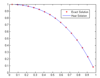
Analytic solution is given by $y(x)=(1-x){{e}^{x}}.$ In Figure 1, exact and approximate solution for $J=3$is represented. The comparison values of absolute errors of the HWCM with Adomian decomposition method (ADM [20]) and Differential transformation method (DTM [15]) is shown in Table 1.
Figure 1. Comparison of approximate and exact solution of Ex. 1
Table 1. Comparison of numerical results of Ex. 1
|
X Exact Approxi Absolute Absolute Absolute solution mate error by error by error by solution HWCM ADM[20] DTM[15] |
|
0.1 0.9947 0.9947 7.1E-15 4.4E-10 4.6E-13 0.2 0.9771 0.9771 8.2E-14 4.9E-10 5.7E-12 0.3 0.9449 0.9449 2.8E-13 7.4E-10 2.1E-11 0.4 0.8951 0.8951 5.7E-13 6.6E-10 4.7E-11 0.5 0.8244 0.8244 8.2E-13 3.0E-1 7.4E-11 0.6 0.7288 0.7288 8.8E-13 4.3E-10 8.9E-11 0.7 0.6041 0.6041 6.9E-13 3.7E-10 7.9E-11 0.8 0.4451 0.4451 3.6E-13 7.3E-10 4.7E-11 0.9 0.2460 0.2460 7.2E-14 7.0E-10 1.1E-11 |
Example 2: Consider the linear BVP of type 1:
${{y}^{(7)}}(x)+y(x)=-{{e}^{x}}(35+12x+2{{x}^{2}}),\ \ \ \ \ x\in (0,\ 1)\ \ \ \ \ $ (35)
with boundary conditions:
$\begin{align} & y(0)\ =0,\ y(1)\ =0,\ {{y}^{(1)}}(0)\ =1,\ {{y}^{(1)}}(1)\ =-e,\ {{y}^{(2)}}(0)\ =0, \\ & \ \ \ \ \ \ \ \ \ \ \ \ \ \ \ \ \ \ \ \ \ {{y}^{(2)}}(1)\ =-4e,\ {{y}^{3}}(0)\ =-3.\ \ \ \ \ \ \ \ \ \ \ \ \ \,\,\,\ \ \ \\ \end{align}$ (36)
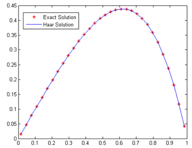
Analytic solution is given by $y(x)=x(1-x){{e}^{x}}.$ In Figure 2, the comparison of exact and Haar solution for $J=4$ is represented. In Table 2, errors obtained by HWCM are compared against the Variation of parameters method (VPM [14]) and Petrov-Galerkin method (PGM [21]).
Figure 2. Comparison of approximate and exact solution of Ex. 2
Table 2. Comparison of numerical results of Ex. 2
|
X Exact Approxi Absolute Absolute Absolute solution mate error by error by error by solution HWCM VPM[14] PGM[21] |
|
0.1 0.0995 0.0995 6.0E-14 8.5E-13 1.4E-07 0.2 0.1954 0.1954 6.9E-13 9.9E-12 6.4E-07 0.3 0.2835 0.2835 2.4E-12 3.5E-11 2.9E-06 0.4 0.3580 0.3580 4.8E-12 7.3E-10 4.4E-06 0.5 0.4122 0.4122 6.9E-12 1.1E-10 6.7E-06 0.6 0.4373 0.4373 7.4E-12 1.3E-10 6.4E-06 0.7 0.4229 0.4229 5.9E-12 1.5E-10 3.7E-06 0.8 0.3561 0.3561 3.0E-12 2.7E-10 3.3E-07 0.9 0.2214 0.2214 6.1E-13 2.2E-09 1.4E-06 |
Example 3: Consider the nonlinear BVP of type 1:
${{y}^{(7)}}(x)=-{{e}^{x}}{{y}^{2}}(x),\ \ \ \ \ x\in (0,\ 1),\ \ \ \ \ \ \ \ \ \ \ \ \ \ \ \ \ \,\,\,\,\,\,\,\,\ \ \ \ \ \ \ \ \ \,\,$ (37)
subject to the boundary conditions:
$\begin{align} & y(0)\ =1,\ \,\,y(1)\ ={{e}^{-1}},\ \,\,{{y}^{(1)}}(0)\ =-1,\ \,\,{{y}^{(1)}}(1)\ =-{{e}^{-1}},\ \\ & {{y}^{(2)}}(0)\ =1,\,\,\,{{y}^{(2)}}(1)\ ={{e}^{-1}},\ \,\,\,{{y}^{3}}(0)\ =-1.\ \ \ \ \ \ \ \ \ \ \ \ \ \ \,\,\,\,\,\,\,\,\,\,\,\ \\\end{align}$ (38)
The exact solution is${{e}^{-x}}$. Using Quasilinearization technique, nonlinear BVP (35) is converted into a sequence of linear BVPs [22], as
$y_{n+1}^{(7)}(x)+2 e^{x} y_{n}(x) y_{n+1}(x)=e^{x}\left[y_{n}(x)\right]^{2}$, (39)
with boundary conditions :
$\begin{align} & {{y}_{n+1}}(0)=1,{{y}_{n+1}}(1)={{e}^{-1}},\ y_{n+1}^{(1)}(0)=-1,y_{n+1}^{(1)}(1)=-{{e}^{-1}}, \\ & \ \ \ \ \ \ \ y_{n+1}^{(2)}(0)=1,y_{n+1}^{(2)}(1)={{e}^{-1}},y_{n+1}^{(3)}(0)=-1.\ \ \ \ \ \ \ \ \ \ \ \ \ \ \ \ \ \ \ \\ \end{align}$ (40)
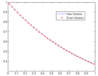
Here ${{y}_{0}}(x)$is chosen from the physical or mathematical perspectives of given problem. We assume that ${{y}_{0}}(x)$ has Maclaurian series expansion. We computed only one iteration i.e. ${{y}_{1}}(x)\approx y(x).$ In Figure 3 comparison of exact and approximate solution for J=5 is represented. Errors obtained by HWCM are compared with ADM [20] and DTM [15] are tabulated in Table 3.
Figure 3. Comparison of approximate and exact solution of Ex. 3
Table 3. Comparison of numerical results of Ex. 3
|
X Exact Approxi Absolute Absolute Absolute solution mate error by error by error by solution HWCM ADM [20] DTM [15] |
|
0.1 0.9048 0.9048 5.5E-16 1.6E-09 3.0E-14 0.2 0.8187 0.8187 4.5E-15 1.6E-09 3.7E-13 0.3 0.7408 0.7408 1.5E-14 4.9E-09 1.4E-12 0.4 0.6703 0.6703 2.8E-14 1.5E-09 3.0E-12 0.5 0.6065 0.6065 3.9E-14 1.5E-09 4.8E-12 0.6 0.5488 0.5488 4.2E-14 2.5E-09 5.7E-12 0.7 0.4966 0.4966 3.2E-14 1.4E-08 5.1E-12 0.8 0.4493 0.4493 1.6E-14 2.5E-09 2.9E-12 0.9 0.4066 0.4066 3.7E-15 5.4E-09 6.9E-13 |
Example 4: Consider the nonlinear BVP of type 2:
${{y}^{(7)}}(x)={{e}^{\text{-}x}}{{y}^{2}}(x),\ \ \ \ \ x\in (0,\ 1),\ \ \ \ \ \ \ \ \ \ \ \ \ \ \ \ \ \ \ \ \ \ \ \ \ \ \ \ \ \ \ \ \ $ (41)
subject to the boundary conditions:
$y(0)=1, y\left(\frac{1}{2}\right)=e^{\frac{1}{2}}, y(1)=e, y^{(1)}(0)=1, y^{(2)}(0)=1 y^{(3)}(0)=1, y^{(4)}(0)=1$ (42)
The exact solution is ${{e}^{x}}.$ By Quasilinearization technique [22], we have
$y_{n+1}^{(7)}(x)=2{{e}^{-x}}{{y}_{n}}(x){{y}_{n+1}}(x)-{{e}^{-x}}{{[{{y}_{n}}(x)]}^{2}},\ \ \ \ \ \ \ \ \ \ \ \ \ \ \ \ \ \ \ $ (43)
with boundary conditions:
$\begin{align} & {{y}_{n+1}}(0)=1,{{y}_{n+1}}(\frac{1}{2})={{e}^{\frac{1}{2}}},\ y_{n+1}^{(1)}(0)=1,y_{n+1}^{{}}(1)=e, \\ & \ \ \ \ \ \ \ y_{n+1}^{(2)}(0)=1,y_{n+1}^{(3)}(0)=1,y_{n+1}^{(4)}(0)=1.\ \ \ \ \ \ \ \ \ \ \ \ \ \ \ \ \ \ \ \ \ \ \ \\ \end{align}$ (44)
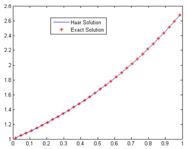
In Figure 4 comparison of exact and approximate solution for J=4 is represented. The errors obtained by HWCM are compared with Homotopy perturbation method (HPM[23]) are in Table 4.
Figure 4. Comparison of approximate and exact solution of Ex. 4
Table 4. Comparison of numerical results of Ex. 4
|
X Exact Approxi mate Absolute Absolute solution solution error by error by HWCM HPM [23] |
|
0.1 1.1052 1.1052 6.7E-16 1.0E-06 0.2 1.2214 1.2214 6.7E-15 4.8E-07 0.3 1.3499 1.3499 3.4E-14 4.9E-06 0.4 1.4918 1.4918 7.3E-14 5.4E-07 0.5 1.6487 1.6487 4.4E-16 6.9E-07 0.6 1.8221 1.8221 5.5E-13 5.6E-07 0.7 2.0138 2.0138 2.3E-12 3.9E-07 0.8 2.2255 2.2255 5.9E-12 4.9E-07 0.9 2.4596 2.4596 9.8E-12 1.5E-06 |
In this paper, we solved seventh order BVPs arise in Mathematical modeling of induction motors with two rotor circuits to test the efficiency of the Haar wavelet method. We have taken few test problems of linear and nonlinear type. Nonlinear problems were solved with the aid of quasilinearization technique. According to convergence analysis as the level of resolution increases, absolute error decreases. Comparison of the numerical results with other methods ensured that the proposed method is more accurate and quite reasonable.
Author Padmanabha Reddy is thankful to Vision Group on Science and Technology, Karnataka Govt., India, for the financial support under the scheme “Seed Money to Young Scientists for Research (SMYSR-FY-2015-16)”. Prof. N. M. Bujurke is grateful to DST [DST/SR/S4/MS: 771/12] for the financial support.
[1] Patrick J. V., “Introduction: Why wavelets,” in Discrete Wavelet Transformations: An Elementary Approach with Applications, New Jersey: John Wiely and Sons, 2007, pp. 1-13.
[2] Lepik U. and Hein H., “Haar wavelets,” Haar Wavelets with Applications, vol. 4, Springer, 2014, pp. 7-20.
[3] Haar A., “Zur theoric der orthogonalen Funktionsysteme,” Math. Annal, vol. 69, pp. 331-371, 1910. DOI: 10.1007/BF01456326.
[4] Chen C. F. and Hsiao C. H., “Haar wavelet method for solving lumped and distributed-parameter systems,” IEEE Proc. Control Theory Appl., vol. 144, pp. 87−94, 1997, DOI: 10.1049/ip-cta:19970702.
[5] Chen C. F. and Hsiao C. H., “ Wavelet approach to optimizing dynamic systems,” IEEE Proc. Control Theory. Appl., vol. 146, pp. 213−219, 1999. DOI: 10.1049/ip-cta:19990516.
[6] Lepik U., “Haar wavelet method for solving higher order differential equations,” Int. J. Math. Comput., vol. 1, pp. 84−94, 2008.
[7] Hariharan G. and Kannan K., “An overview of Haar wavelet method for solving differential and integral equations,” Wl. Appl. Sci. J., vol. 12, pp. 01−14, 2013, DOI: 10.5829/idosi.wasj.2013.23.12.423.
[8] Harpreet K., Mittal R. C. and Vinod M., “Haar wavelet quasilinearization approach for solving nonlinear boundary value problems,” Amer. J. Comp. Math., vol. 1, pp. 176−182, 2011. DOI: 10.4236/ajcm.2011.13020.
[9] Bujurke N. M., ShiralashettI S. and Salimath C., “An application of single-term Haar wavelet series in the solution of nonlinear oscillator equations,” J. Comput. Appl. Math., vol. 227, pp. 234−244, 2009, DOI: 10.1016/j.cam.2008.03.012.
[10] Siraj-ul-Islam, Imran A. and Bozidar S., “The numerical solution of second order boundary value problems by collocation method with the Haar Wavelets,” Math. Comp. Model., vol. 52, pp. 1577−1590, 2010. DOI: 10.1016/j.mcm.2010.06.023.
[11] Fazal-i-Haq, Arshed A. (2011). Numerical solution of fourth order boundary value problems using Haar wavelets, Appl. Math. Sci. [Online]. 63, pp. 3131−3146, http://www.m-hikari.com/ams/ams-2011/ams-61-64-2011/haqAMS61-64-2011.
[12] Fazal-i-Haq, Arshed A. and Iltaf H., “ Numerical solution of sixth-order boundaryvalue problems by collocation method using Haar wavelets,” Appl. Math. Sci., vol. 43, pp. 5729−5735, 2012, DOI: 10.5897/IJPS11.696.
[13] Richrds G. and Sarma P. R. R., “Reduced order models for induction motors with two rotor circuits,” IEEE. Tran. Ener. Conv., vol. 9, pp. 673−678, 1994, DOI: 10.1109/60.368342.
[14] Siddiqi S. S. and Muzammal I. (2013, Jan). “Solution of seventh order boundary value problems by variation of parameters method,” Resae. J . Appl. Sci. Eng. Tech. [Online]. 5, pp. 176−179, http://maxwellsci.com/print/rjaset/v5-176-179.pdf.
[15] Siddiqi S. S., Ghazala A., and Muzammal I. (2012). “Solution of seventh order boundary value problem by differential transformation method,” Wl. Appl. Sci. J. [Online]. 16, pp. 1521−1526, http://www.idosi.org/wasj/wasj16%2811%2912/7.pdf.
[16] Siddiqi S.S., Ghazala A. and Muzammal I. (2012). Solution of seventh order boundary value problems by variational iteration technique. Appl. Math. Sci. [Online]. 6, pp. 4663−4672, Available: http://www.m-
hikari.com/ams/ams-2012/ams-93-96-2012/siddiqiAMS93-96-2012-2.pdf.
[17] Ghazala A. and Hamood R. (2014) “Numerical solution of seventh order boundary value problems using the reproducing kernel space,” Resea. J. Appl. Sci. Eng. Tech.[Online]. 7, pp. 892−896, http://www.maxwellsci.com/print/rjaset/v7-892-896.pdf.
[18] Majak J., Shvartsman B. S., Kirs M., Pohlak M. and Herranen H., “Convergence theorem for the Haar wavelet discretization method,” Composite Structures, vol. 126, pp. 227−232, 2015, DOI:10.1016/j.compstruct.2015.02.050.
[19] Majak J., Shvartsman B., Karjust K., Mikola M., Haavajoe A. and Pohlak M., “On the accuracy of the Haar wavelet discretization method,” Composites part B, vol. 80, pp. 321−327, 2015, DOI:10.1016/j.compositesb.2015.06.008.
[20] Siddiqi S. S. and Muzammal I. (2013). “Solution of seventh order boundary value problems using Adomian decomposition method,” http://arxiv.org/abs/1301.3603v1.
[21] Kasi viswanadham K. N. S. and Reddy S. M., “Numerical solution of seventh order boundary value problems by petrov-galerkin method with quintic B-splines as basis functions and septic B-splines as weight functions,” Int. Jl. Comp. Appl., vol. 122, pp. 0975−8887, 2015, DOI: 10.5120/21700-4811.
[22] Bellman R. E. and Kabala R. E., “Quasilinearization and nonlinear boundary value problems,” Amer. New York: Elsevier, 1965.
[23] Siddiqi S. S. and Muzammal I. (2013) “Use of Homotopy perturbation method for solving multipoint boundary value problems,” http://arxiv.org/abs/1301.2909.