Aeri Rachmad*![]() | Husni
| Husni ![]() | Mohammad Syarief
| Mohammad Syarief ![]() | Eka Mala Sari Rochman
| Eka Mala Sari Rochman ![]() | Yuli Panca Asmara
| Yuli Panca Asmara ![]() | Miswanto
| Miswanto ![]() | Suci Hernawati
| Suci Hernawati ![]()
© 2025 The authors. This article is published by IIETA and is licensed under the CC BY 4.0 license (http://creativecommons.org/licenses/by/4.0/).
OPEN ACCESS
Tuberculosis (TB) continues to pose a significant challenge to global public health, especially in countries with limited healthcare infrastructure. Early identification is key to mitigation; however, the interpretation of microscopic images poses a significant obstacle. This research proposes the use of Deep Learning Models, specifically GoogleNet, for the identification of TB bacteria from microscopic images. The study uses a dataset comprising 1,266 microscopic images to identify TB bacteria. This dataset is then divided into two parts, with 80% of the data used for training (1,012 images) and 20% for testing (254 images). Before being fed into the model, the images are processed using median filter techniques to enhance quality and consistency. This study proposes the use of Deep Learning models, particularly GoogleNet, as a method for detecting TB bacteria in microscopic images. Four optimization algorithms, RMSprop, SGD, Adam, and SGDM, are evaluated and compared to identify the most effective configuration for optimal performance. The experimental findings indicate that the Adam optimizer yields the best results for TB classification. By applying transfer learning techniques, the GoogleNet model is trained and evaluated using standard metrics. The evaluation results demonstrate high accuracy and efficiency in training time. The model achieved excellent accuracy, precision, recall, and F1-Score, each at 98.52%.
tuberculosis bacteria, microscopic images, deep learning, GoogleNet, Adam optimizer
There is still a long way to go in the fight against tuberculosis (TB), but it is especially crucial in countries with low per capita income and poor healthcare infrastructure, where people often have trouble getting medical care [1]. Mycobacterium tuberculosis is the germs that cause this disease. If it is not adequately recognized and treated, it can have major effects on the person's health, as well as on social and economic elements of their life [2]. After trying a lot of different ways to find and cure the condition, one of the biggest problems in the future will be getting an accurate diagnosis [1].
Microbiological bacterial identification on a blood sample [3] is one way to tell if someone has tuberculosis in isolation. The TBC microscopy sample identification approach is quick and cheap. Nevertheless, variability in subjective assessment and heterogeneity in microscopic image quality may adversely affect the accuracy and consistency of the diagnosis [4]. In recent years, new hopes have emerged to overcome this constraint and enhance the efficiency of the initial TBC identification process, especially with the evolution of building-specific technology, particularly Convolutional Neural Networks (CNNs) [5]. In this research, we examined the application of GoogleNet, a CNN, for the bacteriological identification of TBC from microscope pictures. Transfer learning techniques are used to feed the GoogleNet model tiny photos of microorganisms [6]. This lets the model exploit information that is already in the bigger dataset. The evaluation employs conventional criteria in medical research, including anxiety, pressure, recall, and F1-score. This study emphasizes the significance of an optimization approach in assessing model performance, while also addressing architectural layout. The study sought to identify the optimal combination of various algorithms, including RMSprop, SGD, Adam, and SGDM, to enhance the assessment of the model's efficacy in media TB detection.
The research findings indicate that the sampled pattern can detect TBC bacteria with a significant degree of sensitivity. The GoogleNet model can also do better than manual microbiology-based methods when it comes to diagnosing. All of these suggest that CNN with GoogleNet architecture for identifying bacteria using microscopy could be a useful tool for diagnosing and treating TB around the world.
2.1 System architecture
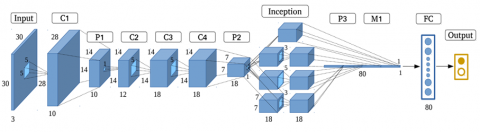
The initial stage in building the architecture in Figure 1 is to take photographs of TB with a microscope. This method makes sure that the data is good enough to be used for further analysis. The following step after taking the picture is preprocessing, which uses a median filter. To get rid of noise in photographs while maintaining crucial information, which is very critical for correct analysis, you apply a median filter.
Figure 1. System diagram
After that, the processed TB dataset will be divided into two parts: 80:20. In this part, 80% will be training data to teach the model, and 20% will be test data to see how well the model works. It is very important to split this dataset so that the model doesn't overfit, which is when it fits too closely to the training data and doesn't generalize well to new data.
Then, the next step is to use a CNN with the GoogleNet architecture to classify the data. GoogleNet was chosen since it has been shown to be able to handle complex image data and complex hierarchical features. GoogleNet uses a structure called an "inception module" that lets the network efficiently extract features from different scales. The inception module lets the network process images with different levels of resolution at the same time by using many parallel paths in one layer. This makes the visual representations richer.
After the classification process is complete, the results will be evaluated thoroughly to measure the accuracy, precision, recall and F1-score value of the model developed. This evaluation will also include the time it takes to classify the entire dataset. This analysis is important for figuring out how well Google's CNN model can classify TB image data while also considering how long it takes to do it.
2.2 Sputum images dataset
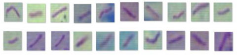
The dataset employed in this study comprises sputum images obtained using a microscope. A total of 1,266 images were successfully collected. The dataset is divided into two classes: 633 images of sputum from TB patients and 633 images from non-TB individuals. Below are examples of TB-positive and TB-negative sputum images as shown in Figure 2 and Figure 3.
Figure 2. Images of tuberculosis individuals
Figure 3. Images of non- tuberculosis individuals
2.3 Median filter on sputum images
The median filter was originally introduced by Tukey [7] and is a nonlinear filtering technique that operates by sliding a narrow window across the image, often with an odd number of pixels [8]. Compared to linear smoothing filters of the same size, it is particularly successful in removing impulsive noise, sometimes known as salt-and-pepper noise [9]. In practice, the filter sorts the pixel values in the window and replaces the center pixel with its median. This method reduces harsh changes, allowing the pixel values to merge more organically with their neighbors. Additionally, the Median Filter can also change the values of isolated pixel groups, which have brightness or darkness levels different from their neighbors and have an area less than n2/2, by using the median value from an nxn matrix. Consequently, the noise removed by the Median Filter will have values similar to the median intensity of its neighboring pixels [8].
Figure 4. Block diagram of the median filter workflow
Figure 4 shows that in the context of the sequence P(1) < P(2) < P(3) < P(n), the statement refers to the process of sorting data elements from the smallest rank (P(1)) to the largest rank (P(n)). In other words, each data element is sorted based on its relative value in the dataset, from smallest to largest as shown in Figure 5. For example, if we have a dataset containing values 3, 7, 1, and 5, after the sorting process, the sequence of values will be 1, 3, 5, and 7. Meanwhile, the value of m corresponds to the formula:
$m=\frac{n+1}{2}$ (1)
where, n = number of data, m = new median value.
Figure 5. Example of median filter application
2.4 Architecture GoogleNet
The main development offered by GoogleNet is its application to a structure known as inception model [10]. Overall, inception adopts the concept of a network within a network, consisting of sub-networks to optimize performance. In the context of image processing, an efficient local structure is rarely applied repeatedly from start to finish to obtain better feature representations. In its application, three types of inception structures tailored to different needs are introduced: generally, 1 × 1 convolutions are used to reduce dimensions before applying more complex 3 × 3 and 5 × 5 convolutions, thereby improving computational efficiency and enhancing feature representation quality. Furthermore, the use of inception modules enables the network to learn hierarchical representations from simple to complex features, with each sub-network focusing on processing different features in the image. This allows the network to be more adaptive and capable of capturing various levels of detail in image data, improving object recognition and classification performance. This network has quite impressive capabilities in classifying patterns from around 1000 images. Additionally, compared to AlexNet, GoogLeNet uses significantly fewer parameters, about 12 times fewer [11]. Like most neural networks used in computer vision contexts, this model takes images as input and produces labels for the classes it learns, along with confidence levels as output [12]. The GoogLeNet architecture consists of a total of 22 layers, which include 9 inception modules. The modified inception modules, as seen in Figure 6, utilize adaptable filters with sizes ranging from (1 × 1) to (5 × 5) to perform convolution in parallel. This approach assists in capturing various levels of detail from the existing features [13].
Figure 6. GoogleNet architecture
2.5 Optimization algorithm
The optimization process in machine learning plays a crucial role as an essential tool to adjust the values of the objective function based on the available data. Through consistent iterative steps, the algorithm continuously updates the model parameters to minimize prediction errors. Thus, the model can continuously learn from the available data and improve its accuracy. This study used four different optimization methods to boost the model's efficiency, which shed light on the ways in which each technique aids in the development of better machine learning algorithms.
RMSprop is a modification of the AdaGrad method that seeks to enhance performance in non-convex scenarios by altering the accumulation of gradients by the application of an exponential moving average. When utilizing a conventional learning rate of 0.001 in Stochastic Gradient Descent (SGD), RMSprop helps fix the problem of the learning rate dropping too quickly. To understand how RMSprop works better, look at how the parameters vary in Eqs. (2)-(4). Gives a general idea of how the RMSprop algorithm updates model parameters depending on the gradients that have been collected [14].
$r=\rho r+(1-\rho) g \odot g$ (2)
$\Delta \theta=\frac{\alpha}{\delta+\sqrt{r}} \odot g$ (3)
$\theta=\theta+\Delta \theta$ (4)
In this instance, r denotes the accumulation of the squared gradient, which is beneficial for modulating parameter updates by considering gradient fluctuations. The parameter p functions as the decay rate, dictating the rate at which the accumulation of the square gradient diminishes with time. The computed parameter update is referred to as ∆θ, representing the modification required for the model parameters. The learning rate, denoted by α, is the magnitude of adjustment applied at each iteration during parameter updates. The constant ẟ, valued at 107, is employed to avert division by zero in the computation. Ultimately, θ represents the first model parameter subject to modification. All these parts collaborate to ensure the model learns from the input effectively and efficiently.
A prominent variant of the gradient descent optimization technique is SGD. In contrast to batch gradient descent, which modifies parameters solely after processing the complete dataset, SGD updates parameters following each unique training example. This regular updating enables the algorithm to converge more rapidly, rendering it particularly advantageous for extensive datasets. Due to its efficiency and responsiveness, SGD is frequently utilized in situations requiring swift parameter modifications, typically with a learning rate of 0.01. The SGD parameter update rule is presented in Eq. (5), which demonstrates the iterative optimization of model parameters utilizing the gradient of an individual data point at each iteration.
$\theta=\theta-\eta * \nabla_\theta \mathrm{J}\left(\theta ; x^i ; y^i\right)$ (5)
Here, θ indicates the parameter that is modified with each iteration of model training, whereas η denotes the learning rate, which determines the magnitude of the adjustment. The pair xi represents the input data and the output data utilized in that phase. In each iteration, the model refines θ utilizing the gradient derived from the data, so enhancing the parameters incrementally with each cycle. In this manner, SGD facilitates the model's continuous enhancement by learning from individual examples, enabling rapid adaptation and effective responsiveness to variations in the training data [14].
Adam is a widely utilized optimization algorithm that integrates concepts from two proven techniques: RMSProp and Momentum. RMSProp incorporates the capability to automatically modify the learning rate for each parameter, hence addressing the prevalent challenge of selecting an appropriate learning rate. Simultaneously, it employs the concept of momentum to ensure updates go in a consistent manner, rather than changing too abruptly. By integrating these two methodologies, Adam renders the optimization process both stable and efficient. This has rendered it one of the most prevalent algorithms in machine learning, facilitating robust performance across various tasks.
$m_i=\beta_1 m_i+\left(1-\beta_1\right) \frac{\partial L}{\partial \theta_i}$ (6)
$v_i=\beta_1 v_i+\left(1-\beta_2\right)\left(\frac{\partial L}{\partial \theta_i}\right)^2$ (7)
In this context, parameter (6) refers to momentum, while parameter (7) represents the exponential moving variance used in the optimization algorithm. Momentum (6) helps speed up convergence by keeping the parameter updates moving in a consistent direction. On the other hand, the exponential moving variance (7) adapts the learning rate for each parameter, making the optimization process more stable and efficient. When the initialization values for time steps and decay rates are too small, parameters (6) and (7) tend to approach a value close to 1, which can introduce bias in the estimation. To mitigate this issue, bias correction and moment estimation are conducted through the division of the parameters in Eqs. (6) and (7) by the difference between 1 and the decay factor. This adjustment stabilizes the moment calculations and produces more accurate estimates.
Implementing this adjustment helps minimize the initial estimation bias, leading to more dependable parameter values throughout the optimization process. This step is essential to ensure consistent and dependable results, especially when dealing with sensitive initial conditions.
$\widehat{m}=\frac{m_i}{1-\beta_1}$ (8)
$\hat{v}=\frac{v_i}{1-\beta_2}$ (9)
Adam, an optimization algorithm proposed by its developers, suggests setting β₁ to 0.9, β₂ to 0.999, and ε to 10⁻⁸. These values were determined through extensive experiments to provide strong performance across a wide range of tasks. In this setup, beta-1 and beta-2 control the exponential moving averages of the gradient and the squared gradient, while epsilon is included to prevent division by zero. After the optimal values for parameters (8) and (9) have been obtained, which represent these moving averages, the Adam update formula can then be applied.
$\theta_{t+1}=\theta_t-\frac{\partial}{\sqrt{v_t+\varepsilon}} \cdot m_t$ (10)
According to its formulation (10), Adam combines the core ideas of RMSProp with the momentum method in gradient estimation to improve both speed and stability during model training. By using the exponential moving average of the gradient together with the exponential moving variance, Adam can adjust the learning rate for each parameter individually. This adaptability gives Adam an advantage over earlier optimization algorithms [15-17].
SGDM is an adaptation of the gradient descent optimization technique that modifies model parameters during the processing of training data. SGDM is distinguished by the use of a momentum factor, which accelerates convergence and mitigates oscillations, especially in the context of extensive datasets. SGDM changes parameters by integrating momentum from prior updates, enabling the model to navigate more smoothly through both flat and steep gradient areas, rather than solely relying on the complete dataset for updates. The standard learning rate for SGD is typically established at 0.01, but this figure may be modified based on the intricacy of the issue.
$\mathrm{Gt}=\nabla_\theta \mathrm{J}\left(\theta ; x^i ; y^i\right)$ (11)
In SGDM, the parameter θ is revised at each step. The learning rate η dictates the magnitude of each update step, whereas xi and yi denote the input-output data pairs utilized in training. With each iteration, θ is modified according to the processed data, enabling the model to progressively enhance its performance by learning from each instance [18].
2.6 Confusion matrix
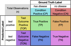
Figure 7 illustrates how the four mentioned values are arranged in the confusion matrix. This version also lists the total number of observations in the top left corner, as well as the marginal counts at the top and left side of the matrix. The colors used for each section of the matrix represent the combination of categories that form the values within it [19]. For example, the color green represents true positives, which consist of false positives and false negatives. Each model has four values that describe its own performance. Therefore, the importance of each of these values must be considered when comparing the overall performance of the models [20]. Classification metrics are calculated from the numbers in the confusion matrix, so to understand these metrics, one must understand the meaning of each value within it [21].
Figure 7. Confusion matrix
True Positive: This means the model correctly detected the disease.
True Negative: This means the model correctly identified that there is no disease.
False Positive: This means the model incorrectly identified someone as having the disease when they actually do not.
False Negative: This means the model failed to detect someone who actually has the disease.
With a confusion matrix, various model performance evaluation metrics can be calculated, such as accuracy, precision, sensitivity (recall), specificity, and F1-score [22]. A confusion matrix is a very useful tool for understanding the performance of a classification model and identifying areas where the model needs improvement. A brief explanation of some commonly used evaluation metrics alongside the confusion matrix [23]:
Accuracy
The percentage of total correct predictions made by the model out of all the test data.
$Accuracy =\frac{\mathrm{TP}+\mathrm{TN}}{\mathrm{TP}+\mathrm{TN}+\mathrm{FP}+\mathrm{FN}}$ (12)
Precision
The percentage of true positive predictions out of all positive predictions made by the model.
$Precision =\frac{\mathrm{TP}}{\mathrm{TP}+\mathrm{FP}}$ (13)
Recall
The percentage of positive data successfully identified by the model out of all the actual positive data.
$Recall =\frac{\mathrm{TP}}{\mathrm{TP}+\mathrm{FN}}$ (14)
F1-Score
The harmonic mean between precision and sensitivity. It is used to compromise between both in one metric.
$F1-Score =2 \mathrm{TP} /(2 \mathrm{TP}+\mathrm{FN}+\mathrm{FP})$ (15)
3.1 Test scenario
The subsequent phase of the research involves training the GoogleNet model on a dataset of TB bacterial pictures derived from microscopic observations. A series of tests was performed using several optimizers, such as Adam, RMSProp, SGD, and SGDM. The batch size was kept at 16, the learning rate was set at 0.0001, and the number of epochs was set to 20 to get the best results. The experimental data are thereafter displayed in tabular format to facilitate further research in the domain of tuberculosis diagnosis by microscopic image analysis, as seen in Table 1 [21].
Table 1. Test scenario [21]
|
|
Optimizer |
Batch |
Learning Rate |
Epoch |
|
Test Scenario |
Adam |
16 |
0.0001 |
20 |
|
RMSProp |
16 |
0.0001 |
20 |
|
|
SGD |
16 |
0.0001 |
20 |
|
|
SGDM |
16 |
0.0001 |
20 |
3.2 Test result
Experimental results related to Tuberculosis show that the GoogleNet model achieves excellent performance when optimized with Adam, employing a learning rate of 0.0001, a batch size of 16, and 20 epochs. The corresponding test results are presented in Figures 8-11.
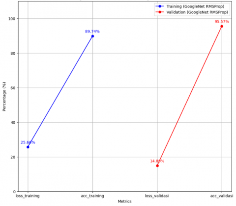
The results presented in Figure 8, obtained using the GoogleNet model with the RMSProp optimizer, indicate that the model attains 89.74% accuracy on the training data, accompanied by a loss of 25.66%. Its performance on the validation data is likewise highly satisfactory, reaching an accuracy of 95.57% and a loss of 14.80%. These outcomes suggest that the model is able to learn from the training data exceptionally well and maintain high performance on the validation data, demonstrating strong generalization capabilities.
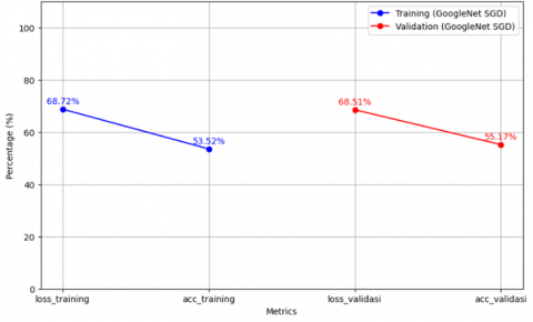
The results presented in Figure 9, obtained using the GoogleNet model with the SGD optimizer, indicate that the model performs reasonably well on the training data, an accuracy of 53.52% and a loss of 68.72% are obtained. In addition, the model demonstrates comparable performance on the validation dataset, with an accuracy of 55.17% and a loss of 68.51%. These findings suggest that the model is successfully learning from the training data and shows stable performance on the validation data, although further improvements are needed to increase accuracy.
Figure 8. RMSProp optimizer trial result graph
Figure 9. SGD optimizer trial result graph
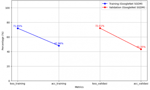
The test results in Figure 10, obtained using the GoogleNet model with the SGDM optimizer, indicate that the model performs reasonably well on the training data, with an accuracy of 47.96% with a loss of 71.85% is achieved. Furthermore, the model demonstrates satisfactory performance on the validation data, reaching an accuracy of 43.35% and a loss of 72.01%. These results suggest that the model can effectively extract meaningful learning patterns from the training data, but still requires further improvements to reduce loss and increase accuracy on both the training and validation data.
Figure 10. SGDM optimizer trial result graph
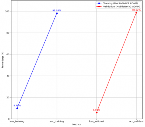
Figure 11. Adam optimizer trial result graph
Regarding the loss, Figure 11 shows a value of 5.80%, reflecting a low error rate during training. Moreover, the model attains an accuracy of 98.52%, demonstrating its strong capability to classify tuberculosis images with high precision. Besides high accuracy, the GoogleNet model also shows excellent results in terms of precision, recall, and F1-Score, each reaching 98.52%. Precision measures the accuracy of the model's positive predictions, while recall measures how well the model finds all positive instances. The F1-Score is the harmonic mean of precision and recall, providing an overall picture of the model's performance in classification. Not only in terms of prediction quality, but the GoogleNet model also demonstrates efficiency in training time. With only about 76.04 seconds required to train the model, it shows that this model is not only accurate and consistent but also efficient in the use of computational resources, as shown in Table 2.
Table 2. Comparison of metric values between the training and validation phases
| Loss | Accuracy | Precision | Recall | F1-Score | Time(s) | |
| Train | 9.74 | 98.03 | 98.06 | 98.03 | 98.03 | 76.04 |
| Validation | 5.8 | 98.52 | 98.52 | 98.52 | 98.52 | 122.81 |
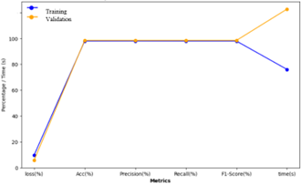
Figure 12. GoogleNet experimental results of metrics between GoogleNet training and validation stages
Figure 12 presents a comparison of the metrics obtained during the training and validation phases, depicting the model's stability and effectiveness in both stages.
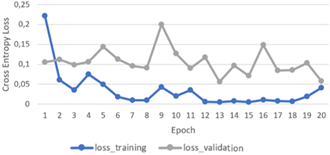
Figure 13 illustrates that the loss curve of the GoogleNet model for TB classification exhibits a consistent decline in training loss values across successive epochs, indicating the model's progress in understanding the data patterns. However, there is variation in the loss on the validation data, suggesting the possibility of overfitting at some points. At Epoch 7, the loss value decreases on both the training and validation data, reflecting good performance on both datasets. Subsequently, at Epoch 12, the training loss value reaches its lowest point, indicating that the model has successfully adapted to the training data. Although there is a slight increase in validation loss at Epoch 12, the model's performance remains high with good accuracy.
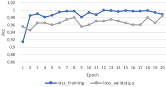
Figure 14 shows a graph depicting the accuracy performance of the GoogleNet model in classifying Tuberculosis bacteria during the training and validation process. The image shows some fluctuations in the accuracy results on the training data and validation results during the epoch. Overall, an increase in accuracy was observed on both data types as the epochs progressed, indicated by the GoogleNet model's increased ability to classify data more accurately. There are several indicators of marked accuracy improvements, showing that the model’s performance has generally improved. The more iterations performed, the higher the accuracy achieved by the GoogleNet model in classifying TB data.
Figure 13. GoogleNet loss performance
Figure 14. GoogleNet accuracy performance
The conclusion from the experimental results indicates that the GoogleNet model excels in TB classification. For this classification task, the Adam optimizer was utilized with a batch size 16, a learning rate of 0.0001, and a total of 20 training epochs. With a loss rate of 5.80% and an accuracy rate of 98.52%, the model demonstrates excellent capability in accurately classifying TB images. Additionally, the model has high precision, recall, and F1-Score, each reaching 98.52%. The performance graph of GoogleNet loss shows a decrease in loss values on the training data from epoch to epoch, indicating the model's progress in understanding the data patterns. Despite some variation in the validation loss, the model's performance remains high with good accuracy. Overall, the graph illustrates the improvement in GoogleNet's accuracy in classifying TB data as the iterations progress.
Future research will focus on implementing layer selection techniques in the CNN architecture to reduce training time and computational costs, while simultaneously improving the overall accuracy and robustness of the model.
We would like to express our sincere gratitude to the Ministry of Higher Education, Science, and Technology (KEMENDIKTISAINTEK) for funding this research through the Fundamental Regular Research (PFR) Grant in 2025. We also extend our appreciation to Universitas Trunojoyo Madura, Universitas Airlangga Surabaya, and INTI International University Malaysia for their valuable collaboration in this research project.
[1] World Health Organization. (2019). Global tuberculosis report 2019. https://www.who.int/publications/i/item/global-tuberculosis-report-2019.
[2] Sugirtha, G.E., Murugesan, G. (2017). Detection of tuberculosis bacilli from microscopic sputum smear images. In 2017 Third International Conference on Biosignals, Images and Instrumentation (ICBSII), Chennai, India, pp. 1-6. https://doi.org/10.1109/ICBSII.2017.8082271
[3] Mithra, K.S., Emmanuel, W.R.S. (2018). FHDT: Fuzzy and hyco-entropy-based decision tree classifier for tuberculosis diagnosis from sputum images. Sādhanā, 43: 125. https://doi.org/10.1007/s12046-018-0878-y
[4] Tamtyas, F.I., Rini, C.S. (2020). The detection of TB lungs with microscopic and the rapid molecular test methods. Medicra (Journal of Medical Laboratory Science/Technology), 3(1): 1-4. https://doi.org/10.21070/medicra.v3i1.650
[5] Rachmad, A., Chamidah, N., Rulaningtyas, R. (2020). Mycobacterium tuberculosis images classification based on combining of convolutional neural network and support vector machine. Communications in Mathematical Biology and Neuroscience, 2020: 85. https://doi.org/10.28919/cmbn/5035
[6] Kumar, S., Arif, T., Alotaibi, A.S., Malik, M.B., Manhas, J. (2023). Advances towards automatic detection and classification of parasites microscopic images using deep convolutional neural network: Methods, models and research directions. Archives of Computational Methods in Engineering, 30(3): 2013-2039. https://doi.org/10.1007/s11831-022-09858-w
[7] Zhu, Y.L., Huang, C. (2012). An improved median filtering algorithm for image noise reduction. Physics Procedia, 25: 609-616. https://doi.org/10.1016/j.phpro.2012.03.133
[8] Qur'ana, T.W. (2018). Perbaikan citra menggunakan median filter untuk meningkatkan akurasi pada klasifikasi motif sasirangan. Technologia: Jurnal Ilmiah, 9(4), 270-279. https://doi.org/10.31602/tji.v9i4.1543
[9] Maulana, I., Andono, P.N. (2016). Analisa perbandingan adaptif median filter dan median filter dalam reduksi noise salt & pepper. Cogito Smart Journal, 2(2): 157-166. https://doi.org/10.31154/cogito.v2i2.26.157-166
[10] Szegedy, C., Liu, W., Jia, Y., Sermanet, P., et al. (2015). Going deeper with convolutions. In 2015 IEEE Conference on Computer Vision and Pattern Recognition (CVPR), Boston, MA, USA, pp. 1-9. https://doi.org/10.1109/CVPR.2015.7298594
[11] Rachmad, A., Syarief, M., Hutagalung, J., Hernawati, S., Rochman, E.M.S., Asmara, Y.P. (2024). Comparison of CNN architectures for Mycobacterium tuberculosis classification in sputum images. Ingénierie des Systèmes d’Information, 29(1): 49-56. https://doi.org/10.18280/isi.290106
[12] Al-Huseiny, M. (2021). Transfer learning with GoogLeNet for detection of lung cancer. Indonesian Journal of Electrical Engineering and computer science. Indonesian Journal of Electrical Engineering and Computer Science, 22(2): 1078-1086. https://doi.org/10.11591/ijeecs.v22.i2.pp1078-1086
[13] He, K., Zhang, X., Ren, S., Sun, J. (2016). Deep residual learning for image recognition. In 2016 IEEE Conference on Computer Vision and Pattern Recognition (CVPR), Las Vegas, NV, USA, pp. 770-778,. https://doi.org/10.1109/CVPR.2016.90
[14] Munir, K., Elahi, H., Ayub, A., Frezza, F., Rizzi, A. (2019). Cancer diagnosis using deep learning: A bibliographic review. Cancers, 11(9): 1235. https://doi.org/10.3390/cancers11091235
[15] Kusumah, H., Zahran, M.S., Rifqi, K.N., Putri, A.D., Hapsari, E.M.W. (2023). Deep learning pada detektor jerawat: Model YOLOv5. Journal Sensi: Strategic of Education in Information System, 9(1): 24-35. https://doi.org/10.33050/sensi.v9i1.2620
[16] Arouri, Y., Sayyafzadeh, M. (2022). An adaptive moment estimation framework for well placement optimization. Computational Geosciences, 26(4): 957-973. https://doi.org/10.1007/s10596-022-10135-9
[17] Kingma, D.P. (2014). Adam: A method for stochastic optimization. arXiv preprint arXiv:1412.6980. https://doi.org/10.48550/arXiv.1412.6980
[18] Yuan, W., Hu, F., Lu, L. (2022). A new non-adaptive optimization method: Stochastic Gradient Descent with Momentum and difference. Applied Intelligence, 52(4): 3939-3953. https://doi.org/10.1007/s10489-021-02224-6
[19] Tharwat, A. (2021). Classification assessment methods. Applied computing and informatics, 17(1): 168-192. https://doi.org/10.1016/j.aci.2018.08.003
[20] Ponraj, A., Nagaraj, P., Balakrishnan, D., Srinivasu, P.N., Shafi, J., Kim, W., Ijaz, M.F. (2025). A multi-patch-based deep learning model with VGG19 for breast cancer classifications in the pathology images. Digital Health, 11: 20552076241313161. https://doi.org/10.1177/20552076241313161
[21] Rachmad, A., Husni, Hutagalung, J., Hapsari, D., Hernawati, S., Syarief, M., Rochman, E.M.S., Asmara, Y.P. (2024). Deep learning optimization of the EfficienNet architecture for classification of tuberculosis bacteria. Mathematical Modelling of Engineering Problems, 11(10): 2664-2670. https://doi.org/10.18280/mmep.111008
[22] Chen, R.C., Dewi, C., Huang, S.W., Caraka, R.E. (2020). Selecting critical features for data classification based on machine learning methods. Journal of Big Data, 7(1): 52. https://doi.org/10.1186/s40537-020-00327-4
[23] Mehdiyev, N., Enke, D., Fettke, P., Loos, P. (2016). Evaluating forecasting methods by considering different accuracy measures. Procedia Computer Science, 95: 264-271. https://doi.org/10.1016/j.procs.2016.09.332