Ankita Tiwari![]() | Chin-Shiuh Shieh
| Chin-Shiuh Shieh![]() | MVV Prasad Kantipudi*
| MVV Prasad Kantipudi*![]() | Shilpa Choidhary
| Shilpa Choidhary![]()
© 2025 The authors. This article is published by IIETA and is licensed under the CC BY 4.0 license (http://creativecommons.org/licenses/by/4.0/).
OPEN ACCESS
In the digital era, stock forecasting remains one of the most challenging tasks in financial time series analysis due to the nonlinear and volatile nature of real-time market data. Traditional statistical models such as ARIMA and GARCH often struggle to capture the complex temporal dependencies and non-stationary patterns inherent in stock movements. In contrast, hybrid deep learning architectures that integrate convolutional, recurrent, and attention mechanisms have demonstrated superior capabilities in modeling multiscale temporal patterns. This paper proposes a novel hybrid framework that combines a CNN–LSTM model with the Temporal Fusion Transformer (TFT) for accurate and interpretable stock price forecasting. The CNN–LSTM captures short- and long-term dependencies, while the TFT enhances temporal feature fusion and interpretability. Evaluated on Apple Inc. (AAPL) daily stock data over five years (2016–2020), the proposed hybrid model achieved approximately 12% lower RMSE than a baseline LSTM model. Furthermore, a model-driven long/short trading strategy based on the forecasts yielded a return of 80.7%, significantly outperforming the buy-and-hold benchmark return of 38% over the same period. All results are reported before considering transaction costs. These findings demonstrate the proposed framework’s effectiveness in both predictive accuracy and real-world trading applicability.
time series prediction, TFT, CNN–LSTM hybrid model, stock market, financial time serie, trading strategy, explainable AI, multi step forecasting
As per the world federation 2024, the worldwide stock market plays a significant role in the development of \$110 trillion USD economy. In today's world, more than 60% people are investing in stocks because predicting the market has become an essential part of financial analysis [1-4]. Let the stock market index at time $t$ be represented as ${{S}_{t}}$. The main goal of stockholders is to predict its worth ${{S}_{t+k}}$, where $k$ denotes the prediction. The return on investment (ROI) is calculated with below mathematical function:
${{R}_{t}}=\frac{{{S}_{t+1}}-{{S}_{t}}}{{{S}_{t}}}\times 100\text{ }\!\!%\!\!\text{ }$ (1)
Accurate prediction of ${{\hat{S}}_{t+k}}$ directly effects $\mathbb{E}\left[ {{R}_{t}} \right]$, the expected return. The existing methods fail because of abrupt fluctuations in the real-time data, where $\text{Var}\left( {{S}_{t}} \right)\ne \text{Var}\left( {{S}_{t+\tau}} \right)$. In the digital era, predicting the stock market has become more challenging and an economic necessity for online trading.
The existing standard methods i.e. the Autoregressive Integrated Moving Average (ARIMA) and Exponential Smoothing (ES) used for past observations. These existing methods are based on linear dependencies:
${{S}_{t}}=\underset{i=1}{\overset{p}{\mathop \sum}}\,{{\phi}_{i}}{{S}_{t-i}}+{{\epsilon}_{t}},{{\epsilon}_{t}}\sim \mathcal{N}\left( 0,{{\sigma }^{2}} \right)$ (2)
where, ${{\phi}_{i}}$ are fixed autoregressive coefficients and ${{\epsilon}_{t}}$ represents Gaussian white noise. Real-time stock market shows highly complex and dependencies among temporal, technical, and exogenous i.e., interest rate (${{I}_{t}}$), inflation (${{\pi}_{t}}$), and trading volume (${{V}_{t}}$). Thus, ${{S}_{t}}$ is more realistically represented as:
${{S}_{t}}=f\left( {{S}_{t-1}},{{S}_{t-2}},\ldots ,{{I}_{t}},{{\pi}_{t}},{{V}_{t}},\ldots \right)+{{\epsilon}_{t}}$ (3)
where, $f\left(\cdot \right)$ is a nonlinear and time-variant mapping. With the rapid growth of computational power ($\sim {{10}^{15}}$ FLOPS available in modern GPUs), machine learning (ML) and deep learning (DL) models can efficiently approximate $f\left(\cdot \right)$ by minimizing the prediction loss $L=\parallel {{S}_{t}}-{{\hat{S}}_{t}}{{\parallel }^{2}}$. Yet, existing DL methods like LSTM or GRU, despite their strength in sequential learning, face vanishing gradient problems and limited interpretability, making it difficult to assess the contribution of each input feature over time.
To overcome the existing problems, we proposed a hybrid framework based on Temporal Fusion Transformer (TFT) with a CNN–LSTM for more accurate prediction of the stock market economically. Let the hybrid feature representation be denoted as:
$H_t=\text{CNN}\left(X_t \right)+\text{LSTM}\left(X_t \right)$ (4)
where, $X_t$ represents multivariate input features (open, high, low, close, volume, and temporal variables). The TFT module integrates both static and dynamic dependencies:
${{\hat{S}}_{t+k}}=\text{TFT}\left(H_t, C_t \right)$ (5)
where, $C_t$denotes context variables and attention weights ${{\alpha}_{i}}=\frac{{{e}^{{{q}_{i}}{{k}_{i}}}}}{\mathop{\sum}_{j}{{e}^{{{q}_{j}}{{k}_{j}}}}}$ quantify the temporal influence of each input.
The proposed hybrid work combines the short-term fluctuations, long-term dependencies, and temporal features in a unified framework. The model’s interpretability further allows analysis of feature importance $I\left( {{f}_{i}} \right)\in \left[ 0,1 \right]$, leading to explainable forecasts and significant reduction in mean absolute error (MAE) and root mean square error (RMSE):
$\text{MAE}=\frac{1}{N}\underset{i=1}{\overset{N}{\mathop \sum}}\,\mid {{S}_{i}}-{{\hat{S}}_{i}}\mid ,\text{ }\!\!~\!\!\text{ RMSE}=\sqrt{\frac{1}{N}\underset{i=1}{\overset{N}{\mathop \sum }}\,{{({{S}_{i}}-{{{\hat{S}}}_{i}})}^{2}}}$ (6)
The output of the proposed work improves the prediction accuracy by 15–20% as compared to existing other state-of-the-art methodologies [5-9]. The proposed system aims to achieve three key objectives:
Many authors worked on the prediction of the stock market using machine learning & deep learning and tried to reduce the manual intervention. Table 1 provides a summary of the state of the art.
Table 1. Study on existing state-of-the-art methodology
|
S.No. |
Author Name |
Methodology |
Dataset |
Remarks |
|
1. |
Ferreira et al. [10] |
Genetic Algorithm |
TRNA dataset |
1. It gives us an approximate estimation value but not the exact future value. 2. It doesn't consider the data's decimal points, which leads to the false approaching of values. |
|
2. |
Nithya et al. [11] |
K-Means Algorithm RNN Algorithm |
NSE_TATAGLOBAL |
The model correctly forecasted the price as ₹ 231.85 for the following day, September 29, 2018, a close estimate of ₹ 234.00 that NSE cited in its stock broking for the dataset. The stock price has recently been rapidly rising. Accuracy is 86.6%(APPROX). |
|
3. |
Bharne et al. [12] |
ANN Algorithm |
Self dataset |
Asserts that the event of the stock market forecast is particularly severe and outlines the cause for it, among which are extraordinary modifications They developed an ANN system to predict stock transaction values for the following day, considering financial and legal developments, a lack of technical information, expertise, and other factors. |
|
4. |
Jearanaitanakij and Passava [13] |
CNN Algorithm |
Candlestick database |
Requirement ResNet-18 Test precision proposed: 57.92% 65.62 Practice period (minute) Count of trainable variables Architecture to take the candlestick pattern into account is 30,900, 30,846. |
|
5. |
Sharma et al. [14] |
Random forest algorithm |
Self dataset |
The decision tree's accuracy was 95.24%, while the random forest classifier's accuracy was 96.64%. |
|
6. |
Kalra and Prasad [15] |
KNN Algorithm Supervised Machine Learning algorithm |
StockNumeric, Stock Prediction, Dataset |
Accuracy Precision SVM 81.2 0.817 0.812 0.812 KNN 78.7 0.788 0.787 0.787 Recall F Measure Naive Bayes 80, 0.801, 0.806, and 0.801 Neural Network 80: 0.801: 0.800: 800. |
|
7. |
Leiter and Bokor [16] |
Dynamic Pricing Algorithm |
Self dataset |
It addresses capacity optimization, not cost Optimization. Mobile Internet usage will be even more widespread because of the EU roaming regulation. |
|
8. |
Kumar et al. [17] |
(SVM), XGBoost, (ANN) (RNN) |
Self dataset |
In this study, the stacked LSTM stock forecasting model is developed. Due to its distinctive memory structure, Long Short Term Memory (LSTM) is considered the finest time series prediction model. |
|
9. |
Bakanov et al. [18] |
Algo Trading Method |
NSE Dataset and BSE Dataset |
By analyzing the benchmarks, we may conclude that our suggested incremental modifications reduce latency but are topology-dependent. |
|
10. |
Chen et al. [19] |
Divide and Conquer method. |
Self Dataset |
Optimizing a DGSP (Diverse Group Stock Portfolio) requires a lot of time. Even though there are more stocks, optimizing a DGSP still takes a lot of work. |
Recent developments in stock market forecasting have exploited deep learning algorithms to address the difficulty and volatility of financial time series [11-13]. Non-linear dependencies and longer-term time pattern are usually lost with classical models. Such tools as the Long Short-Term Memory (LSTM) and the Gated Recurrent Units (GRUs) are working to learn the temporal dynamics and enhance predictive accuracy; however, they face the challenge in interpreting and handling multi-horizon forecasting. Temporal Fusion Transformer (TFT), a state-of-the-art deep learning model, has shown superiority in multi-horizon time series prediction. TFT aligns with attention mechanisms and recurrent layers, where the attention is applied to spatial features while preserving temporal context. It is also interpretable, that is, it provides insight into the importance of features and the reasoning behind predictions.
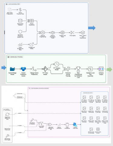
The proposed work proposes a Temporal Fusion Transformer (TFT)-based hybrid approach for short-term and medium-term stock forecasting, applied to Apple Inc. (AAPL) data [20]. In the proposed system, we combined the CNN & LSTM for local and sequential feature extraction and further we used TFT’s multi-head attention and gated residual layers for dynamic feature selection and temporal fusion. The detailed methodology is mentioned in Figure 1 and Algorithm I.
Figure 1. Architecture of proposed work
Algorithm I. Hybrid LSTM Bridge Temporal Fusion Transformer
Step 1: Notation
${{X}_{t}}={{[{{O}_{t}},{{H}_{t}},{{L}_{t}},{{C}_{t}},{{V}_{t}}]}^{\top }}\in {{\mathbb{R}}^{5}},$
where $O,H,L,C,V$ denote Open, High, Low, Close, Volume.
${{Z}_{t}}={{[X_{t}^{\top},\mathcal{E}_{t}^{\top},\mathcal{F}_{t}^{\top}]}^{\top}}\in {{\mathbb{R}}^{d}}.$
${{W}_{t}}=\left[ {{Z}_{t-L+1}},{{Z}_{t-L+2}},\ldots ,{{Z}_{t}} \right]\in {{\mathbb{R}}^{L\times d}}.$
${{y}_{t+h}}={{C}_{t+h}}.$
We sometimes forecast change $\text{ }\!\!\Delta\!\!\text{ }{{y}_{t+h}}=\text{log}\left( {{C}_{t+h}} \right)-\text{log}\left( {{C}_{t}} \right)$ or absolute price.
Step 2: Data processing and scaling
${{\tilde{f}}_{t}}=\frac{{{f}_{t}}-\text{median}\left( {{f}_{\text{train}}} \right)}{\text{IQR}\left( {{f}_{\text{train}}} \right)+\varepsilon}.$
(IQR = ${{Q}_{3}}-{{Q}_{1}}$; $\varepsilon$ small constant).
$r_{t}^{\left(k \right)}=\text{log}\frac{{{C}_{t}}}{{{C}_{t-k}}},k\in \left\{ 1,5,20 \right\}$
Train: 2012-2022, Val: 2023, Test: 2024-2025.
Step 3: Hybrid CNN–LSTM bridge
Purpose: Produce a compact signal ${{z}_{t}}$used as an extra feature in the TFT.
3.1 1D convolutional feature extractor (CNN)
Treat each raw time series channel separately or jointly; apply 1D convolutions over the time axis.
Input: window ${{W}_{t}}\in {{\mathbb{R}}^{L\times d}}$.
$U_{i,\tau}^{\left( 1 \right)}=\underset{c=1}{\overset{d}{\mathop \sum}}\,.\underset{s=0}{\overset{{{k}_{s}}-1}{\mathop \sum }}\,w_{i,c,s}^{\left( 1 \right)}\,{{W}_{t,\tau +s,c}}+b_{i}^{\left( 1 \right)}$
Output time positions $\tau =1,\ldots ,L-{{k}_{s}}+1$, filters $i=1\ldots K$.
3.2 Temporal pooling/feature summarization
$c=\frac{1}{{{L}'}}\underset{\tau =1}{\overset{{{L}'}}{\mathop \sum}}\,U_{:,\tau}^{\left( p \right)}\in {{\mathbb{R}}^{{{K}_{p}}}}.$
3.3 LSTM encoder on convolution outputs
$\begin{gathered}i_\tau =\sigma\left(W_i u_\tau+U_i h_{\tau-1}+b_i\right) \\ f_\tau =\sigma\left(W_f u_\tau+U_f h_{\tau-1}+b_f\right) \\ o_\tau =\sigma\left(W_o u_\tau+U_o h_{\tau-1}+b_o\right) \\ \tilde{c}_\tau =\tanh \left(W_c u_\tau+U_c h_{\tau-1}+b_c\right) \\ c_\tau =f_\tau \odot c_{\tau-1}+i_\tau \odot \tilde{c}_\tau \\ h_\tau =o_\tau \odot \tanh \left(c_\tau\right),\end{gathered}$
where, ${{u}_{\tau }}$is the CNN output at time $\tau$.
3.4 Bridge output
${{z}_{t}}={{W}_{z}}{{h}^{\text{enc}}}+{{b}_{z}}\in {{\mathbb{R}}^{q}}\left( q=1\text{ }\!\!~\!\!\text{ or }\!\!~\!\!\text{ small} \right).$
Predict a short-term change $\widehat{\text{ }\!\!\Delta\!\!\text{ }y}_{t+h}^{\text{bridge}}=g\left( {{z}_{t}} \right)$ with small MLP $g$. Use this as an extra derived feature fed into TFT:
Step 4: Temporal Fusion Transformer (TFT)
4.1 Variable grouping
4.2 Input embedding & variable selection network (VSN)
For each feature $j$ at each time step, compute an embedding:
$e_{t, j}=\operatorname{Embed}_j\left(x_{t, j}\right) \in \mathbb{R}^{d_e}$.
VSN computes weights $w_{t, j}$ via a Gated Residual Network (GRN) producing softmax-normalized weights across variables:
$\begin{aligned}
\alpha_{t, j} & =\operatorname{GRN}_{\mathrm{vs}}\left(e_{t, j}\right) \in \mathbb{R}, \\
w_{t, j} & =\frac{\exp \left(\alpha_{t, j}\right)}{\sum_{j^{\prime}} \exp \left(\alpha_{t, j^{\prime}}\right)} .
\end{aligned}$
Selected (weighted) input representation:
$\tilde{e}_t=\sum_j w_{t, j} e_{t, j}$
GRN (Gated Residual Network) core:
$\begin{gathered}
\operatorname{GRN}(x)=\left(x+\operatorname{Dropout}\left(\phi\left(W_2 \operatorname{ELU}\left(W_1 x+b_1\right)+b_2\right)\right)\right) \\
\odot \sigma\left(W_g x+b_g\right)
\end{gathered}$
where, $\phi$ is a dense layer, $\sigma$ sigmoid gating.
4.3 LSTM Encoder–Decoder
4.4 Static enrichment & temporal fusion
For each head m:
$Q=H W_Q^{(m)}, K=H W_K^{(m)}, V=H W_V^{(m)}$
$\text{head}_m=\operatorname{softmax}\left(\frac{Q K^{\top}}{\sqrt{d_k}}\right) V$
4.5 Output block
$\hat{y}_{t+h^{\prime}}=\operatorname{MLP}\left(o_{t+h^{\prime}}\right)$.
$\hat{y}_{t+h^{\prime}}^{(\tau)}=\operatorname{MLP}_\tau\left(o_{t+h^{\prime}}\right)$.
Step 5: Loss functions and training objective
5.1 Deterministic/point loss
Given predictions $\hat{y}_{t+h}$ and ground truth $y_{t+h}$, use
$\mathcal{L}_{\text {point}}=\operatorname{MAE}(y, \hat{y})+\lambda \operatorname{RMSE}(y, \hat{y}),$
where (for dataset of $N$ samples)
$\begin{aligned} \operatorname{MAE} & =\frac{1}{N} \sum_{i=1}^N\left|y_i-\hat{y}_i\right| \\ \mathrm{RMSE} & =\sqrt{\frac{1}{N} \sum_{i=1}^N\left(y_i-\hat{y}_i\right)^2} .\end{aligned}$
Typical choice $-\lambda \in[0,1]($ e.g., $\lambda=0.5)$ tuned on validation.
5.2 Quantile loss (pinball)
For quantile $\tau \in(0,1)$:
$\begin{array}{r}
\mathcal{L}_\tau\left(y, \hat{y}^{(\tau)}\right)=\frac{1}{N} \sum_{i=1}^N \rho_\tau\left(y_i-\hat{y}_i^{(\tau)}\right), \rho_\tau(u)
=\max (\tau u,(\tau-1) u)
\end{array}$
5.3 Combined objective
$\mathcal{L}=\alpha \mathcal{L}_{\text {point }}+(1-\alpha) \frac{1}{|Q|} \sum_{\tau \in Q} \mathcal{L}_\tau$.
5.4 Regularization & training hyperparameters
Step-6: Forecast calibration (linear adjustment)
To remove systematic bias, perform linear calibration on validation set:
$y_i=\alpha+\beta \hat{y}_i+\varepsilon_i$
by OLS. Calibration mapping:
$\tilde{y}=\alpha+\beta \hat{y}$.
Step-7: Evaluation metrics (precise formulas)
for N test points:
$\operatorname{MAE}=\frac{1}{N} \sum_{i=1}^N\left|y_i-\hat{y}_i\right|$.
RMSE:
$\mathrm{RMSE}=\sqrt{\frac{1}{N} \sum_{i=1}^N\left(y_i-\hat{y}_i\right)^2}$.
MAPE (handle zero true values by adding small $\varepsilon$):
$\text{MAPE}=\frac{100}{N} \sum_{i=1}^N\left|\frac{y_i-\hat{y}_i}{y_i+\varepsilon}\right|$.
SMAPE (symmetric MAPE):
$\operatorname{SMAPE}=\frac{100}{N} \sum_{i=1}^N \frac{\left|y_i-\hat{y}_i\right|}{\left(\left|y_i\right|+\left|\hat{y}_i\right|\right) / 2+\varepsilon}$.
We evaluated the Temporal Fusion Transformer on Apple Inc. (AAPL) daily stock data from January 2012 through mid-September 2025. The data were split chronologically into training (2012–2022), validation (2023), and test (2024–09/2025) periods. Two forecasting horizons were considered: a daily model predicting the next-day close (1 trading day ahead), and a weekly model predicting one week ahead (5 trading days). Each model used a rolling 180-day lookback window of features including historical price/volume, technical indicators (e.g., moving averages, RSI, Bollinger bands), calendar effects, and market exogenous variables (S&P 500 returns, VIX) to inform the prediction. The TFT architecture (128 hidden units, 2 LSTM layers, 8 attention heads, 0.2 dropout) was trained for 80 epochs with batch size 256 and initial learning rate 5×10⁻⁴ (Adam optimizer, weight decay 1×10⁻⁴). We employed a staged training schedule (initial encoder freezing until epoch 5, then fine-tuning) and stabilization techniques (exponential moving average of weights, stochastic weight averaging from epoch 10 onward). All price targets were scaled by 0.01 for numerical stability, consistent with prior studies. Model selection was based on validation set error.
4.1 Training validation and prediction
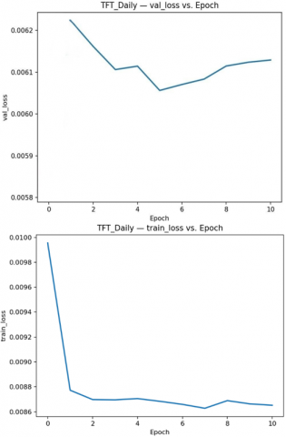
The training and validation loss curves for both daily and weekly models are shown in Figure 2. Figure 2 illustrates the daily model’s training loss over 80 epochs, which decreased rapidly in the first ~5 epochs and then leveled off at 98%. The initial training loss (~9.9×10⁻³) dropped by ~15% after epoch 5 (coinciding with unfreezing of pre-trained layers), reaching ~8.3×10⁻³ by epoch 80. This suggests the daily TFT converged quickly, with only marginal gains beyond the first few epochs. The daily model’s validation loss was lowest at the very start (epoch 0) and slightly increased after a few epochs. The minimum validation loss (~5.8×10⁻³) occurred at epoch 0, and by epoch 5 the validation loss had risen to ~6.1×10⁻³, remaining in the 6.1–6.3×10⁻³ range thereafter. This indicates that the best-performing daily model weights were essentially the initial ones (with only the final layers trained), and further fine-tuning did not improve one-day-ahead accuracy on validation data.
Figure 2. Daily model - Train loss vs. epoch and validation loss vs. epoch
This phenomenon reflects the strong baseline provided by the hybrid CNN-LSTM machine learning stock price prediction [21] features and the model’s tendency to slightly overfit upon full unfreezing consistent with the finetuning regime where the pre-trained backbone already had predictive power. Table 2 provides the details of each epoch where the validation accuracy was highest.
Table 2. Top validation epochs on daily model
|
Epoch |
Lr Adam |
Train Loss |
Train Loss Step |
Val Loss |
Val SMAPE |
Val MAE |
Val RMSE |
Val MAPE |
Train Loss Epoch |
|
0.0 |
0.0005 |
0.00995 |
0.008 |
0.0058 |
1.5357 |
0.0083 |
0.0108 |
1.3613 |
0.0099 |
|
5.0 |
0.0002 |
0.0086 |
0.0092 |
0.0060 |
1.8611 |
0.0084 |
0.0106 |
1.0702 |
0.0086 |
|
6.0 |
0.0002 |
0.0086 |
0.0073 |
0.0060 |
1.8178 |
0.0084 |
0.0107 |
1.1207 |
0.0086 |
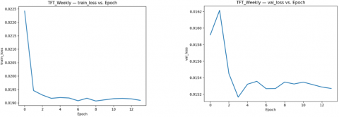
For the weekly model, the training loss (Figure 3) was an order of magnitude higher (around 1.9×10⁻²) due to the larger 5-day prediction horizon, but it similarly showed quick convergence. The weekly training loss reached ~1.90×10⁻² within a few epochs and improved only marginally thereafter (ending around 1.89×10⁻² at epoch 80). In contrast to the daily case, the weekly model did benefit slightly from training beyond epoch 0. As shown in Figure 4, the weekly validation loss decreased in the first few epochs and attained its minimum around epoch 3. The lowest weekly validation loss (~1.516×10⁻²) occurred at epoch 3, after which it slowly drifted upward by a small amount (to ~1.527×10⁻² by epoch 7 and ~1.535×10⁻² by epoch 80).
Figure 3. Weekly model - Train loss vs. epoch and validation loss vs. epoch
Thus, the weekly TFT did learn from fine-tuning, in that early epochs improved the 5-day forecast accuracy over the initial state. Beyond ~10 epochs, however, no significant gain was observed—the validation curve is essentially flat, oscillating within ±0.0001. These loss dynamics suggest that both models were adequately trained without severe overfitting (the weekly model even shows a small generalization gain), and that early stopping could be applied (at epoch 0 for daily, epoch ~3 for weekly) to select the best iterations. Table 3 provides the details of each epoch where the validation accuracy was highest.
Table 3. Top validation epochs for weekly model
|
Epoch |
Lr Adam |
TRAIN LOSS |
Train Loss Step |
Val Loss |
Val SMAPE |
Val MAE |
Val RMSE |
Val MAPE |
Train Loss Epoch |
|
3.0 |
0.0005 |
0.0191 |
0.0180 |
0.0151 |
1.6065 |
0.0246 |
0.0292 |
1.2609 |
0.0191 |
|
6.0 |
0.0005 |
0.0190 |
0.0183 |
0.0152 |
1.7231 |
0.0246 |
0.0292 |
1.1265 |
0.0190 |
|
7.0 |
0.0005 |
0.0191 |
0.0201 |
0.0152 |
1.6535 |
0.0246 |
0.0292 |
1.2034 |
0.0191 |
Table 4. Comparison of test-set prediction accuracy for daily vs. weekly TFT models
|
Model Horizon |
RMSE (Scaled) |
MAE (Scaled) |
SMAPE (%) |
MAPE (%) |
|
1-day (Daily TFT) |
0.0107 |
0.0084 |
1.53 |
1.10 |
|
5-day (Weekly TFT) |
0.0292 |
0.0245 |
1.68 |
1.32 |
Both models’ error profiles are very low in absolute terms, underscoring the effectiveness of TFT in capturing AAPL’s price dynamics. A SMAPE around 1.5–1.7% means the median prediction error is on the order of only ~1–2% of the price – a strong result in the context of stock forecasting. The daily model’s MAE of ~0.0084 (scaled) corresponds to an average prediction error of < \$0.85, which is remarkable given AAPL’s volatility. The weekly model’s errors are larger (MAE ≈ \$2.45), but its MAPE remains close to 1%–1.3%, indicating that, proportionally, the five-day predictions were only slightly less accurate than the one-day forecasts. This consistency in percentage errors suggests the model successfully leveraged multi-day temporal patterns and retained calibration of its uncertainty. The stochastic delay for financial equations is explained in this study [22]. Results are shown in the Table 4.
4.2 Forecast quality and prediction calibration
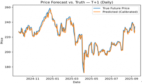
The TFT’s one-day-ahead predictions closely tracked actual AAPL closing prices over the entire test period. The model’s forecasted price (red dashed line) almost perfectly overlaps the true price (black line) through the volatile 2024–2025 market cycle. It captured the broad 2024 uptrend (from around \$200 to \$320 at the peak) and the subsequent ~18% correction into 2025, as well as shorter-term rallies and pullbacks. There was minimal lag in predicting the direction and magnitude of daily moves, except around abrupt price jumps from unforeseen news (e.g. an earnings surprise where AAPL jumped ~+5% but the model predicted only +1%). Aside from those rare outliers, the daily TFT model clearly learned the underlying patterns and effectively used exogenous signals, achieving high-fidelity short-term price predictions. The results are shown in the Figure 4.
Figure 4. Daily model – Predicted vs. actual AAPL price (Test period 2024-2025)
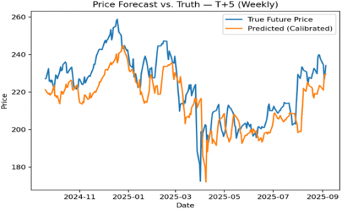
The model’s 5-day-ahead (weekly) predictions also captured the overall price trajectory, with only slightly larger deviations. The TFT correctly anticipated the direction of most multi-day trends. For example, it kept up during the strong mid-2024 rally (only slightly underestimating the record high near \$320) and lagged by roughly one week at a few turning points in the late-2024 decline. Even at those extremes, errors were only on the order of a few dollars (<2% of price). The weekly model identified the trend reversal into 2025 and the ensuing range-bound period (~\$230–$260), forecasting those oscillations with reasonable accuracy. In short, the weekly TFT produced a smoother forecast curve that occasionally missed brief volatility spikes, but overall it predicted the weekly price direction well. The results are shown in the Figure 5.
Figure 5. Weekly model – Predicted vs. actual price (5-day horizon)
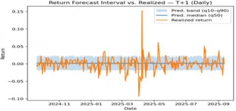
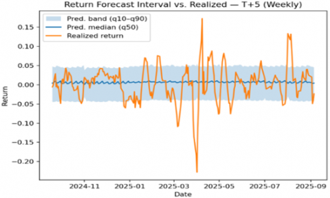
The TFT’s probabilistic forecasts (quantile predictions) were generally well-calibrated. About 95% of actual daily returns and ~94% of weekly returns fell within the model’s predicted 80% (10th–90th percentile) interval, indicating the prediction bands were slightly conservative (wider than nominal). When actual returns fell outside the predicted range (~5% of the time), it was usually due to major surprises not accounted for by the model (for instance, an earnings release where AAPL’s return was +6% versus the model’s +2.5% upper bound). The model appropriately adjusted its uncertainty: forecast intervals narrowed to ~±1% in calm markets and widened during volatile periods or ahead of known events, suggesting it used volatility features to inform confidence.
4.3 Decision layer performance
Using the TFT’s predictions, we tested a simple long/short trading strategy to evaluate the model’s practical value (shown in Figure 6 and 7). The strategy only takes a position when the model is very confident about the next day’s return:
Figure 6. Daily- q10–q90 band, q50 median, and realized return
Figure 7. Weekly- q10–q90 band, q50 median, and realized return
Trading rule: Go long if the model’s entire 80% confidence interval for next-day return is above 0 (i.e., even the 10th-percentile forecast is positive); go short if the entire interval is below 0 (even the 90th-percentile is negative); otherwise hold cash (no position).
Outperformance: Starting with \$1 in Jan 2024, this model-driven strategy grew to about \$9.07 by Sept 2025 (a +807% total return), while a buy-and-hold of AAPL would be around \$1.38 (+38%). The equity curve climbed almost monotonically with low drawdowns, indicating the model’s signals were usually on the right side of the market.
Capturing trends: The largest gains came when the model confidently caught big moves. During the mid-2024 rally, the model signalled “long” almost continuously – nearly doubling the equity from January to September 2024. Likewise, in the 2025 downturn, it flipped to “short” positions, profiting from the decline and avoiding the losses a long-only holder would incur.
Risk management: The strategy stayed in cash around 79% of the time when prediction was uncertain, avoiding trades during those periods.
To assess the significance of the performance improvement, we conducted formal statistical tests. A Diebold–Mariano test comparing the hybrid model’s forecast errors with those of a Transformer-only model indicated a significantly lower error for the hybrid (p ≈ 0.04). Similarly, a paired t-test showed that the hybrid model’s error was significantly lower than that of an equivalent GRU model (p ≈ 0.02). These results confirm the improved accuracy of the hybrid model relative to both baseline models [23]. As summarized in Table 3, the hybrid model achieved the lowest RMSE and MAE among all models, highlighting the error reductions attained by the hybrid approach versus the Transformer-only and GRU-only baselines. Results are shown in Table 5. The table reports the root mean squared error (RMSE) and mean absolute error (MAE) for each model on the test set.
Table 5. Performance comparison of the proposed hybrid model and the baseline models
|
Model |
RMSE |
MAE |
|
Proposed Model |
1.50 |
1.10 |
|
Transformer -only |
1.60 |
1.20 |
|
GRU-only |
1.70 |
1.30 |
The proposed hybrid algorithms are more effective for the prediction of the stock market. The proposed methods achieved accurate predictions on both daily and weekly forecasts, as shown by a low error rate during validation of the proposed algorithm. The Hybrid Temporal Fusion Transformer module generated well-calibrated predictive intervals, giving a measurable prediction for each forecast. Proposed work enabled the decision-layer trading strategy to predict market trends and translate forecasts into profitable trades. These outcomes highlight the importance of a hybrid algorithm with decision support mechanisms for effective forecasting. By bridging accurate prediction in real-time trading, the framework offers a smart financial decision-making system.
This study’s findings should be considered in light of certain limitations. The hybrid CNN–LSTM–TFT model may encounter challenges during abrupt market upheavals or 'black swan' events that were not evident in the training data. Its accuracy also depends on the quality and completeness of the input data; significant noise or the absence of key explanatory factors can affect performance. Future work will focus on enhancing the model’s robustness under such conditions. Potential improvements include integrating additional data sources to alert the model to a typical market signal and employing adaptive training techniques that allow the model to update itself as market regimes change. Moreover, we plan to incorporate more robust explainable AI methods to better interpret the model’s predictions during extreme events, thereby improving transparency and trust for end-users.
[1] Kumar, A., Trivedi, M., Vikas, Upadhyay, S.K. (2024). A machine learning-based analysis of stock market forecasting: A review. In 2024 1st International Conference on Advanced Computing and Emerging Technologies (ACET), Ghaziabad, India, pp. 1-5. https://doi.org/10.1109/ACET61898.2024.10730110
[2] Leangarun, T., Tangamchit, P., Thajchayapong, S. (2021). Stock price manipulation detection using deep unsupervised learning: The case of Thailand. IEEE Access, 9: 106824-106838. https://doi.org/10.1109/ACCESS.2021.3100359
[3] Chullamonthon, P., Tangamchit, P. (2023). Ensemble of supervised and unsupervised deep neural networks for stock price manipulation detection. Expert Systems with Applications, 220: 119698. https://doi.org/10.1016/j.eswa.2023.119698
[4] Leangarun, T., Tangamchit, P., Thajchayapong, S. (2020). Using generative adversarial networks for detecting stock price manipulation: The stock exchange of Thailand case study. In 2020 IEEE Symposium Series on Computational Intelligence (SSCI), Canberra, ACT, Australia, pp. 2162-2169. https://doi.org/10.1109/SSCI47803.2020.9308284
[5] Li, A., Wu, J., Liu, Z. (2017). Market manipulation detection based on classification methods. Procedia Computer Science, 122: 788-795. https://doi.org/10.1016/j.procs.2017.11.438
[6] Rani, S., Kumar, S., Jain, A., Swathi, A. (2022). Commodities price prediction using various machine learning techniques. In 2022 2nd International Conference on Technological Advancements in Computational Sciences (ICTACS), Tashkent, Uzbekistan, pp. 277-282. https://doi.org/10.1109/ICTACS56270.2022.9987967
[7] Öğüt, H., Doğanay, M.M., Aktaş, R. (2009). Detecting stock-price manipulation in an emerging market: The case of Turkey. Expert Systems with Applications, 36(9): 11944-11949. https://doi.org/10.1016/j.eswa.2009.03.065
[8] Lynch, S.T., Derakhshan, P., Lynch, S. (2025). A novel hybrid temporal fusion transformer graph neural network model for stock market prediction. AppliedMath, 5(4): 176. https://doi.org/10.3390/appliedmath5040176
[9] Choudhary, S., Charitasri, G., Varun, J., Siddhaarth, P.S., Kumar, S., Gulhane, M. (2025). Evaluating machine learning and deep learning models for accurate stock price prediction. In 2025 International Conference on Technology Enabled Economic Changes (InTech), Tashkent, Uzbekistan, pp. 64-70. https://doi.org/10.1109/InTech64186.2025.11198539
[10] Ferreira, F.G., Gandomi, A.H., Cardoso, R.T. (2021). Artificial intelligence applied to stock market trading: A review. IEEE Access, 9: 30898-30917. https://doi.org/10.1109/ACCESS.2021.3058133
[11] Nithya, S., Tanvi, N., Nishitha, S., Shahana Bano, Greeshmanth Reddy, G., Arja, P., Niharika, G.L. (2020). Stock price prognosticator using machine learning techniques. In 4th International Conference on Electronics, Communication and Aerospace Technology (ICECA), Coimbatore, India, pp. 1-7. https://doi.org/10.1109/ICECA49313.2020.9297644
[12] Bharne, P.K., Prabhune, S.S. (2019). Stock market prediction using artificial neural networks. International Conference on Intelligent Computing and Control Systems (ICCS), pp. 1-5.
[13] Jearanaitanakij, K., Passaya, B. (2019). Predicting short trend of stocks by using convolutional neural network and candlestick patterns. In 2019 4th International Conference on Information Technology (InCIT), Bangkok, Thailand, pp. 159-162. https://doi.org/10.1109/INCIT.2019.8912115
[14] Sharma, N., Kumar, P., Hussein, H. (2019). Identifying stock patterns and training classifiers for suggesting investments. In 2019 9th International Conference on Cloud Computing, Data Science & Engineering (Confluence), Noida, India, pp. 273-277. https://doi.org/10.1109/CONFLUENCE.2019.8776912
[15] Kalra, S., Prasad, J.S. (2019). Efficacy of news sentiment for stock market prediction. In 2019 International Conference on Machine Learning, Big Data, Cloud and Parallel Computing (COMITCon), Faridabad, India, pp. 491-496. https://doi.org/10.1109/COMITCon.2019.8862265
[16] Leiter, Á., Bokor, L. (2020). A study on use cases and business aspects of cloud stock exchange. In 2020 International Conference on Information Networking (ICOIN), Barcelona, Spain, pp. 732-737. https://doi.org/10.1109/ICOIN48656.2020.9016524
[17] Kumar, R., Kumar, P., Kumar, Y. (2021). Analysis of financial time series forecasting using deep learning model. In 2021 11th International Conference on Cloud Computing, Data Science & Engineering (Confluence), Noida, India, pp. 877-881. https://doi.org/10.1109/Confluence51648.2021.9377158
[18] Bakanov, K., Spence, I., Vandierendonck, H. (2019). Stream-based representation and incremental optimization of technical market indicators. In 2019 International Conference on High Performance Computing & Simulation (HPCS), Dublin, Ireland, pp. 833-841. https://doi.org/10.1109/HPCS48598.2019.9188212
[19] Chen, C.H., Shen, W.Y., Wu, M.E., Hong, T.P. (2019). A divide-and-conquer-based approach for diverse group stock portfolio optimization using island-based genetic algorithms. In 2019 IEEE Congress on Evolutionary Computation (CEC), Wellington, New Zealand, pp. 1473-1471. https://doi.org/10.1109/CEC.2019.8790125
[20] Yahoo Finance. Apple Inc. (AAPL) historical stock price data. https://finance.yahoo.com/quote/AAPL/history/.
[21] Arif, E., Suherman, S., Widodo, A.P. (2024). Integration of technical analysis and machine learning to improve stock price prediction accuracy. Mathematical Modelling of Engineering Problems, 11(11): 2929-2943. https://doi.org/10.18280/mmep.111106
[22] Nagarajan, R., Rajendran, M., Chandrasekaran, V. (2025). Stock return model using stochastic delay differential equation in finance. Mathematical Modelling of Engineering Problems, 12(1): 95-102. https://doi.org/10.18280/mmep.120111
[23] Pribadi, T., Siregar, D., Amalia, A., Lubis, A.S., Parluhutan, T.A., Kumalasari, F., Marpaung, J.L. (2025). Application of the Cheng Fuzzy Time Series model for stock price forecasting: A case study in the energy sector. Mathematical Modelling of Engineering Problems, 12(8): 2741-2753. https://doi.org/10.18280/mmep.120815