Ritzkal*![]() | Pulung Nurtantio Andono
| Pulung Nurtantio Andono![]() | Heru Agus Santoso
| Heru Agus Santoso![]() | Muljono
| Muljono![]()
© 2025 The authors. This article is published by IIETA and is licensed under the CC BY 4.0 license (http://creativecommons.org/licenses/by/4.0/).
OPEN ACCESS
This study evaluates the effectiveness of the Synthetic Minority Over-sampling Technique (SMOTE) in improving machine learning classification of global plastic pollution levels. Using seven common algorithms: Decision Trees, Random Forests, K-Nearest Neighbors (KNN), Support Vector Machines (SVM), Naïve Bayes, AdaBoost, and Logistic Regression, two experimental scenarios were tested: before and after applying SMOTE to a dataset of 212 countries with seven key features. Results show that SMOTE significantly improves the performance of most models, particularly KNN and Random Forest, achieving accuracy above 80% with balanced F1 scores across all classes. SMOTE effectively addresses class imbalance, enabling more accurate identification of minority pollution categories. However, Naïve Bayes and Logistic Regression experienced a slight performance decline due to sensitivity to synthetic data distribution. Overall, integrating SMOTE with standard preprocessing enhances model fairness and generalization, providing actionable insights for global pollution risk classification and supporting data-driven environmental policies.
plastic pollution classification, SMOTE, class imbalance, environmental data analysis, machine learning
Plastic pollution remains one of the most urgent and critical environmental challenges on a global scale [1]. The production of plastic is on the rise annually, and waste management has not been optimized, resulting in pervasive degradation, particularly in marine ecosystems and coastal areas [2]. The accumulation of waste in waters and microplastic pollution have had a significant impact on human health and biodiversity [3]. Current research indicates that there is a necessity for interventions and innovations in plastic waste management technologies, as well as a heightened global awareness of the environmental and health consequences of plastic waste [4]. The issue is further exacerbated by the disparities between countries in terms of recycling capacity, production, and consumption. Developing countries are frequently under significant pressure to address the accumulation of waste, whereas developed countries generate substantial quantities of refuse despite the existence of more sophisticated management systems [5]. Therefore, there is a pressing necessity for a data-driven methodology to identify the characteristics and hazards of plastic debris in various countries. In 2024, global plastic waste reached approximately 220 million tons, with an average of 28 kg per capita, of which 69.5 million tons were poorly managed and entered the environment, threatening terrestrial and marine ecosystems. By 2025, global thermoplastic production is projected to reach 445 million metric tons, with packaging alone accounting for over 140 million metric tons per year [6].
The United States produces more than 42 million tons of plastic waste annually, followed by India (10.2 million tons) and Indonesia (3.4 million tons) [6]. Alarmingly, 80% of plastic waste in the ocean comes from five Asian countries China, Indonesia, the Philippines, Vietnam, and Thailand due to high population density, rapid consumption growth, and inadequate waste management systems [6]. The top 10 list also includes other significant countries, including Brazil, Mexico, and Japan, with an estimated plastic waste volume of 4 to 3.8 million tons, respectively [7]. This demonstrates that nations with concentrated populations and substantial economies generate an exceptionally high volume of plastic refuse.
However, this list also includes a number of European and Southeast Asian countries, including Germany (3,568,313 tons), Indonesia (3,366,941 tons), Thailand (3,355,763 tons), and Italy (3,335,851 tons) [7]. The significant challenges in waste management in the Southeast Asian region are exemplified by the fact that Indonesia and Thailand are among the largest plastic waste producing countries. Overall, this data underscores the necessity of international initiatives to reduce plastic waste and improve waste management in order to mitigate the increasing environmental consequences of plastic pollution.
Classification is essential for the comprehension and management of plastic waste, in addition to aggregation [8, 9]. By examining factors such as the total plastic waste produced, the primary sources of plastic waste, recycling rates, and per capita waste, classification algorithms can be employed to classify countries according to their susceptibility to coastal plastic pollution. This method enables stakeholders to identify priority areas for intervention and develop targeted waste management policies by classifying countries into specific risk categories (e.g., high, medium, low). These supervised learning techniques offer predictive insights that surpass descriptive analysis and facilitate proactive environmental decision-making [10]. This research employs a variety of well-known classification algorithms, such as Naive Bayes, Decision Tree, Extreme Gradient Boosting (XGBoost), Random Forest, K-Nearest Neighbors (KNN) [11], and Decision Tree [12]. Each algorithm possesses its own unique characteristics in terms of robustness, interpretability, and accuracy [13]. Confusion matrices and critical metrics, including precision, recall, accuracy, and F1-score, are implemented to assess the functionality of these classifiers [14]. In order to deduce meaningful conclusions about the plastic waste situation in various countries, these models combine the strengths of dimensionality reduction, clustering, and classification, thereby enhancing the overall analytical framework. Ultimately, the classification results offer actionable information that promotes the sustainability of littoral areas and the improvement of environmental governance.
This research uses various well-known classification algorithms, such as Naive Bayes, Decision Tree, AdaBoost, Random Forest, K-Nearest Neighbors (KNN), Logistic Regression and Decision Tree. Each algorithm has its own unique characteristics in terms of robustness, interpretability, and accuracy. Confusion matrices and important metrics, including precision, recall, accuracy, and F1-score, were implemented to assess the functionality of these classifiers. To draw meaningful conclusions about the situation of plastic waste in different countries, these models combine the strengths of dimensionality reduction, clustering, and classification, thereby enhancing the overall analytical framework. Ultimately, the classification results offer actionable information that promotes continued improvement in environmental governance.
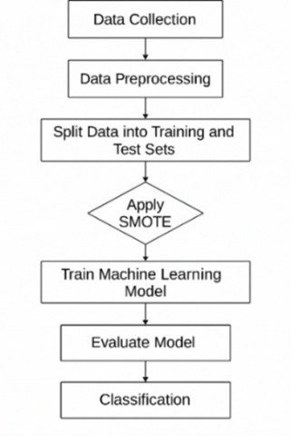
Figure 1. Proposed model for a classification approach to plastic waste
Machine learning-based classification method to identify waste categories based on available datasets. The stages in this research method are described in Figure 1 as follows:
(a) Dataset and data acquisition
This research begins with the use of a waste dataset obtained from trusted data sources, either environmental agencies, open data publications, or survey results. This dataset includes various features that represent waste characteristics such as type, volume, and source of origin.
(b) Pre-processing
Before the data is used for model training, a pre-processing stage is required to ensure data quality and suitability. The steps taken include: Data cleaning: Removing duplicate data and correcting inconsistent values.
1) Missing values handling: Blank or incomplete data is filled in using techniques such as mean, mode, or median imputation, depending on the type of data.
2) Encoding categorical variables: Non-numeric variables are converted into a numeric format using techniques such as Label Encoding or One-Hot Encoding.
3) Normalization or Standardization: Numerical data is normalized using methods such as Min-Max Scaling or StandardScaler to ensure all features are on a comparable scale.
(c) Feature extraction
At this stage, important features of the data are extracted or transformed to improve classification performance. This technique is used to reduce data dimensionality, increase feature relevance, and minimize redundancy.
(d) Handling data imbalance (data balancing with SMOTE)
1) Class imbalance often occurs in classification datasets, where some classes have much less data than others. To address this, the research was conducted in two scenarios:
2) Using SMOTE (Synthetic Minority Over-sampling Technique): This technique creates synthetic data on minority classes by interpolating between nearest neighbor data. This helps balance the amount of data between classes, so that the model is not biased towards the majority class.
3) Not Using SMOTE: For benchmarking purposes, the model is also trained on the original data without the balancing technique so that the performance of both scenarios can be evaluated objectively.
(e) Separation of training and test data
The dataset is divided into training data (80%) and test data (20%). This division aims to train the model on most of the data and test its performance against data that has never been seen before, so that the validity of the generalization can be evaluated objectively.
(f) Classification methods
Several classification algorithms were selected to identify waste types based on the pre-processed features. The algorithms used are:
1) Decision Tree: A decision tree algorithm that divides data based on simple rules and generates a tree structure.
2) Random Forest: An ensemble of many decision trees combined to improve accuracy and reduce overfitting.
3) K-Nearest Neighbors (KNN): A distance-based method that classifies data based on its nearest neighbors.
4) Support Vector Machine (SVM): A classification algorithm that searches for the optimal hyperplane to separate data classes.
5) AdaBoost: A boosting method that combines multiple weak models into a strong model with iterative weighting.
6) Logistic Regression: A statistical model to predict the probability of a class based on a linear combination of input features.
7) Naïve Bayes: A probabilistic model based on Bayes' Theorem with the assumption of independence between features.
(g) Performance evaluation
After model training, evaluation is performed using test data. Several metrics are used to measure the performance of each model:
1) Accuracy: The proportion of correctly classified data out of the total test data.
2) Precision: The ability of the model to correctly identify the positive class (true positives compared to false positives).
3) Recall: The ability of the model to capture all data from the positive class (true positives compared to false negatives).
4) F1 Score: Harmonized average of precision and recall, used when data is not balanced.
5) ROC/AUC (Receiver Operating Characteristic / Area Under the Curve): A metric to measure the discriminative ability of the model against various classification thresholds.
6) Confusion Matrix: A matrix that shows the number of correct and incorrect predictions for each class, providing a more detailed insight into the classification error.
This stage describes the steps in carrying out the process or the results of applying a research method including.
3.1 Dataset
The dataset used is a public dataset which is taken from the World Population Review where the data taken is in 2024. The attributes taken in the data consist of 7 attributes and 212 data. 212 data from country data and 7 attributes consisting of flagCode, country, PlasticPollution_MismanagedWasteIndex_pct_2024, PlasticPollution_TotalPlasticConsumption_2023, PlasticPollution_MismanagedWasteExpected_tons_2023, PlasticPollution_PerCapitaPlasticConsumption_2023, PlasticPollution_MWILevel_text_20232. The description of the seven can be explained in Table 1.
The 7 attributes or features have basic dataset data types which will be described in Table 2.
Table 1. Description of the attributes
|
No. |
Attribute |
Description |
|
1 |
Flag Code |
A numeric or symbolic code used to mark a particular condition or status of the data. The code may indicate data validity, country record type, or entity identification (e.g. countries with incomplete or estimated data). |
|
2 |
Country |
Indicates the name of the country or administrative region that is the object of observation in the dataset. |
|
3 |
PlasticPollution_MismanagedWasteIndex_pct_2024 |
This variable indicates the index of the percentage of mismanaged plastic waste in 2024. |
|
4 |
PlasticPollution_TotalPlasticConsumption_2023 |
Indicates the total plastic consumption of a country in 2023, usually measured in tons or kilograms. |
|
5 |
PlasticPollution_MismanagedWasteExpected_tons_2023 |
This variable represents the estimated amount of plastic waste that is not expected to be properly managed in 2023, measured in tons. |
|
6 |
PlasticPollution_PerCapitaPlasticConsumption_2023 |
Presents data on per capita plastic consumption in 2023, usually in kilograms per person. |
|
7 |
PlasticPollution_MWILevel_text_20232 |
This variable is categorical and describes the level of the mismanaged waste index (MWI) in text or classification, such as “low”, ‘medium’, “high”, or other categories. This value is a qualitative interpretation of the MWI quantitative data, used to facilitate understanding and policy analysis. |
Table 2. World Population Review basic dataset
|
No. |
Attribute |
Description |
|
1 |
Flag Code |
Categorical |
|
2 |
Country |
Categorical |
|
3 |
PlasticPollution_MismanagedWasteIndex_pct_2024 |
Numerical |
|
4 |
PlasticPollution_TotalPlasticConsumption_2023 |
Numerical |
|
5 |
PlasticPollution_MismanagedWasteExpected_tons_2023 |
Numerical |
|
6 |
PlasticPollution_PerCapitaPlasticConsumption_2023 |
Numerical |
|
7 |
PlasticPollution_MWILevel_text_20232 |
Categorical |
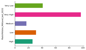
Figure 2. Graph showing the risk level of waste
Figure 2 shows the distribution of plastic pollution levels based on the PlasticPollution_MWLevel_tex_20232 category. This category is divided into five levels: Very Low, Low, Medium, High, and Very High. The graph is presented in the form of a horizontal bar chart, with the length of the bars representing the amount or frequency of data in each category. Based on the graph, there are five types of levels:
(a) Very High has the highest frequency, approaching 100, indicating that most of the regions or data analyzed are at a very high level of plastic pollution.
(b) Followed by the Very Low category with approximately 40, indicating that while some areas have managed to keep plastic pollution levels low, their numbers are still far fewer compared to the “Very High” category.
(c) The Low and High categories are each around 30 and 25, respectively, indicating moderate contributions to the overall distribution.
(d) The Medium category has the smallest number, around 15, indicating that only a few areas are at a moderate level of plastic pollution.
3.2 Pre-processing
Before proceeding with preprocessing, the first step is to check the data type of the labels or features used. The data type checking process for each column in a DataFrame uses the pandas library in Python. This process is an important part of the data preprocessing stage in data analysis and machine learning model development.
Data type checking aims to ensure that each column in the dataset has a data type that is appropriate for the purpose of analysis or modeling. Based on Table 3, the dataset consists of 212 data points and 8 labels or features. The information displayed includes the name of the label or feature, the number of non-null values, and the data type (dtype) of each label/feature. Some labels or features, such as PlasticPollution_TotalPlasticConsumption_2023, PlasticPollution_PerCapitaPlasticConsumption_2023, and Plastic pollution category, are already of type int64, indicating that the values in those columns are integers and ready for numerical processing. However, there are still labels or features with the object data type, such as PlasticPollution_MismanagedWasteIndex_pct_2024 and PlasticPollution_MismanagedWasteExpected_tons_2023, which ideally should also be numeric (int or float) for quantitative analysis purposes. The country and PlasticPollution_MWILevel_text_20232 columns are of type object because they contain categorical data. Detecting these data types is crucial because errors in data types can cause errors in mathematical calculations, misinterpretations, or model training failures. Therefore, the next step in this process typically involves converting data types using data encoding methods, as well as handling missing values. The next step in data preprocessing is encoding categorical variables into numerical form so they can be used in machine learning algorithms. In this study, one of the features that underwent encoding was PlasticPollution_MWILevel_text_20232, which provides information on plastic pollution levels across all countries.
Table 3. Basic data types
|
No. |
Label Name |
Data Type |
|
1 |
flagCode |
Object |
|
2 |
country |
Object |
|
3 |
PlasticPollution_MismanagedWasteIndex_pct_2024 |
Object |
|
4 |
PlasticPollution_TotalPlasticConsumption_2023 |
Int64 |
|
5 |
PlasticPollution_MismanagedWasteExpected_tons_2023 |
Object |
|
6 |
PlasticPollution_PerCapitaPlasticConsumption_2023 |
Int64 |
|
7 |
PlasticPollution_MWILevel_text_20232 |
Object |
|
8 |
Plastic pollution category |
Int64 |
Table 4. Preprocessing encoding
|
No. |
Country |
PlasticPollution_MWILevel_text_20232 |
Plastic Pollution Category |
|
1 |
United States |
Very Low |
0 |
|
2 |
Japan |
Very Low |
0 |
|
3 |
United Kingdom |
Very Low |
0 |
|
… |
…. |
… |
… |
|
210 |
TO |
219 |
3 |
|
211 |
Cayman Islands |
High |
3 |
|
212 |
Northern Mariana Islands |
High |
3 |
In the data preprocessing process, converting categorical data into numerical data is a crucial step to enable machine learning algorithms to perform mathematical calculations efficiently. Table 4 shows that the feature or class PlasticPollution_MWILevel_text_20232, which originally contained categorical labels such as “Very Low” and “High,” has been encoded into numerical values in the new feature or class Plastic pollution category. This process is known as label encoding, where each unique category is assigned a different integer representation. For example, the “Very Low” category is converted to 0, while “High” is converted to 3. These numerical values are then used as input features in classification or regression algorithms. This encoding process is performed using the apply (categorize_plastic_pollution) function, which appears to be a custom function designed to map plastic pollution levels into numerical categories according to a predefined classification scheme. This conversion not only simplifies data processing but also enables pattern learning between numerical variables during model training. This step is an integral part of the preprocessing pipeline in data science and machine learning.
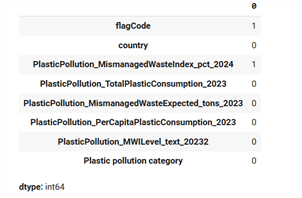
The next step in preprocessing is missing value checking. This check is a very important initial step to ensure data quality before it is used in further analysis or machine learning modeling.
In Figure 3(a), missing values are checked using the dataset.isnull().sum() function, which identifies the number of entries with null values (NaN) in each column. Based on the results displayed, there are two columns containing missing values: flagCode: 1 missing value and PlasticPollution_MismanagedWasteIndex_pct_2024: 1 missing value. Meanwhile, other columns such as country, PlasticPollution_TotalPlasticConsumption_2023, and other numeric columns do not have missing values (marked with the number 0). This indicates that, overall, the dataset is fairly clean, with only a small portion of the data requiring further handling. The identification and handling of missing values aim to prevent statistical bias, computational errors, or even failures in predictive model training. Some common approaches that can be applied after this detection stage include:
(a) Statistical imputation (e.g., using the mean, median, or mode) for numeric columns.
(b) Imputation with specific categories or constants for categorical columns.
(c) Row deletion (if the number of missing values is small and does not significantly impact the data distribution).
(a)
(b)
Figure 3. (a) Results of missing data identification; (b) Handling missing values
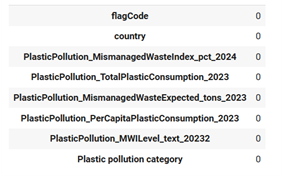
By knowing the location and number of missing values, data analysts can formulate handling strategies that are appropriate for the characteristics of each variable, thereby ensuring that the subsequent analysis process is valid and efficient.
Figure 3(b) illustrates one of the important stages in data preprocessing, namely handling missing values. In the data preprocessing process, detecting and handling missing values is a crucial step to ensure the integrity and quality of data before it is used in statistical analysis or machine learning modeling. In this figure, it is shown that the PlasticPollution_MismanagedWasteIndex_pct_2024 column has missing values and has been handled using the mean imputation method with the following formula.
$\bar{x}=\frac{1}{n} \sum_{i=1}^n X_i$
Description:
$\bar{x}$: mean
$X_i$: value i in the column (not empty)
N:amount of data that is not missing (non-missing)
3.3 Feature extraction
The feature extraction process used to filter a feature, where this process is used for efficiency/model interpretation in this stage, employs feature scaling, which adjusts the numerical values of features to fall within a specific range or distribution, such as having a mean of 0 and a standard deviation of 1 (StandardScaler), or a scale of [0, 1] (MinMaxScaler). This process aims to standardize the scale across numerical variables so that machine learning algorithms, such as Support Vector Machine (SVM), K-Nearest Neighbors (KNN), and AdaBoost, can operate optimally.
$z=\frac{x-\mu}{\sigma}$
Description :
$x$ is the original value
$\mu$ is the average of that column
$\sigma$ is the standard deviation of that column
$z$ is the scaled value (z-score)
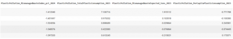
After transformation, the values of each feature will have a mean of 0 and a standard deviation of 1, which helps the model converge faster and not be affected by the dominance of features with large scales in Figure 4.
Figure 4. Results after feature scaling
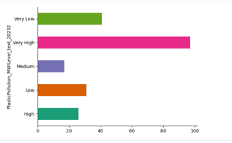
Figure 5 shows the results of Exploratory Data Analysis (EDA), which is the initial stage of data processing aimed at evaluating the structure, patterns, and anomalies in the dataset before further modeling. Figure 5 displays a horizontal bar chart representing the frequency distribution of categories in the PlasticPollution_MWILevel_text_20232 variable, which is the classification of plastic pollution levels based on the Mismanaged Waste Index. This visualization provides important information about the proportion of categories, which consist of: Very High, High, Medium, Low, and Very Low. From the graph, it can be observed that:
(a) The Very High category has the most entries, indicating that most countries in the dataset are at a very high level of plastic pollution.
(b) The Medium category has the fewest data points.
(c) There is an imbalance in the distribution between categories (class imbalance) that can affect the performance of the classification algorithm if not addressed.
Figure 5. Results of the Exploratory Data Analysis (EDA) process
3.4 Handling data imbalance (data balancing with SMOTE)
SMOTE is a data augmentation method known for generating synthetic data using k-nearest neighbors and uniform probability distributions. In the initial process, SMOTE works to separate data distributed to the majority and minority classes. In the next process, each minority class data will have a number of k-neighbors using the k-nearest neighbor (k-NN) method. During the creation of synthetic samples, each minority sample has a nearest neighbor randomly selected from among the k-nearest neighbors.
The application of the SMOTE technique (Synthetic Minority Over-sampling Technique) from the imbalanced-learn library to address class imbalance in a plastic pollution dataset.
Table 5 shows the results of applying the SMOTE (Synthetic Minority Over-sampling Technique) method to a dataset with an imbalanced class distribution in the Plastic Pollution Category. Before the SMOTE process was performed, the total number of samples in the dataset was 211, with a highly imbalanced class distribution. The details of the class distribution before SMOTE show that class 4 dominates with 96 samples, while the other classes have significantly fewer samples, such as class 0 with 41 samples, class 1 with 31 samples, class 3 with 26 samples, and class 2 with only 17 samples. This imbalance has the potential to cause bias in the classification model, where the model tends to be more accurate for the majority class and ignores the minority class. To address this issue, the SMOTE method was applied, which synthetically generates new samples in classes with fewer samples by utilizing interpolation from existing data. After applying SMOTE, the total number of samples increased significantly to 480, and the distribution across classes became balanced, with 96 samples each. This indicates that SMOTE successfully equalized the data across all target classes, namely classes 0, 1, 2, 3, and 4. The application of SMOTE is particularly important in the context of machine learning, especially for classification problems with imbalanced data. With a balanced class distribution, the classification model has a greater chance of learning patterns from each class fairly, resulting in better prediction performance and avoiding bias toward specific classes. The implementation of SMOTE is a strategic step in the data preprocessing stage to ensure the quality and validity of the classification model to be built.
Table 5. Comparison of testing results before and after using SMOTE
|
Class |
Before SMOTE |
After SMOTE |
|
4 |
96 |
96 |
|
3 |
41 |
96 |
|
2 |
31 |
96 |
|
1 |
26 |
96 |
|
0 |
17 |
96 |
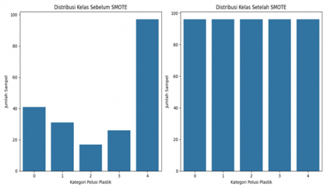
Figure 6. Class distribution before and after SMOTE
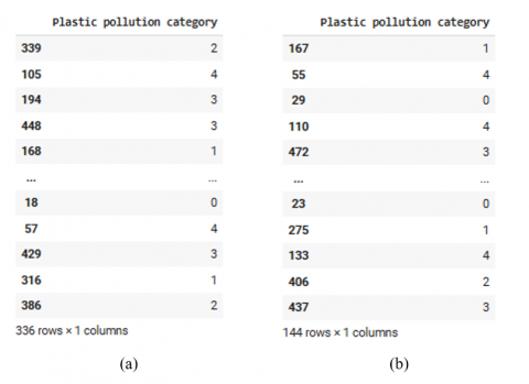
The oversampled data is then divided into a training set and a testing set using a 70:30 ratio, with the parameter stratify=y_resampled to maintain balanced class proportions in each data subset. The results of this division show that the training data consists of 336 samples, while the test data consists of 144 samples. The class distribution in the training data shows that each class has a very balanced number, with the number of samples ranging from 67 to 68. A similar pattern is observed in the test data, with each class having 28 to 29 samples.
Figure 6 shows the Class Distribution Before SMOTE, which indicates that the data exhibits a significant class imbalance. The plastic pollution category labeled 4 has the largest number of samples, nearly reaching 100, while other categories, such as labels 2 and 3, have significantly fewer samples, with less than 30 samples each. Such imbalances are very common in real-world classification problems and can lead to model bias toward the majority class, negatively impacting the model's accuracy and sensitivity toward the minority class. The Class Distribution After SMOTE shows a significant change after the oversampling process using SMOTE. All plastic pollution categories (0 to 4) now have an equal number of samples, each around 96 samples. These results indicate that SMOTE successfully synthesized synthetic data for minority classes, thereby balancing the data distribution proportionally.
Overall, this process demonstrates the effective application of the SMOTE method in enhancing minority class representation without causing information loss or direct overfitting. The resulting balanced class distribution will have a positive impact on the performance of the classification model to be built, as the model no longer tends to dominate the majority class but can recognize patterns from all classes evenly. This technique is particularly important in plastic pollution classification studies, which naturally have classes with unbalanced representation in the initial data.
3.5 Separation of training data and test data
The dataset splitting process is an important step in developing machine learning models to separate training and testing data proportionally and representatively. Based on Figure 7, the data is split using the train_test_split function from sklearn.model_selection library with a 70:30 ratio, where 336 data points are used for training and 144 for testing. This process also utilizes the stratify parameter to maintain a balanced distribution of target classes between training and testing data, which is crucial in multi-class classification, such as in the plastic pollution category. The features used are
a) PlasticPollution_MismanagedWasteIndex_pct_2024,
b) PlasticPollution_TotalPlasticConsumption_2023,
c) PlasticPollution_MismanagedWasteExpected_tons_2023, and
d) PlasticPollution_PerCapitaPlasticConsumption_2023
These features were normalized using standard scaling techniques, resulting in numerical values with a mean distribution of zero and a standard deviation of one. The target labels, representing plastic pollution categories, are presented in numerical form (0–4), reflecting a multi-class classification approach. This step ensures that the model can learn from representative data and be tested on previously unseen data, thereby enhancing the validity of the evaluation and reducing the risk of overfitting.
Figure 7. Results of dataset splitting: (a) Results of the plastic pollution category in the training data; (b) Results of the plastic pollution category in the testing data
3.6 Classification
This classification technique uses seven algorithms, including KNN, Random Forest, Decision Tree, SVM, ADABOOST, Naive Bayes, and Logistic Regression. At this stage, a comparison of these seven algorithms will be reported with the process before using SMOTE and after using SMOTE.
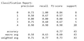
1) Classification of decision tree algorithms
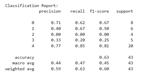
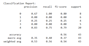
Figure 8(a) illustrates the performance of the model before SMOTE was applied. It can be seen that the data distribution is highly imbalanced, with the majority class (class 4) having 20 data points, while the minority classes (such as classes 2 and 3) only have 4–5 data points. The model's accuracy is 0.63, and the macro average F1-score is only 0.45, indicating that the model is unable to recognize minority classes effectively. Class 2 has a precision, recall, and f1-score of 0.00, meaning that the model did not successfully predict this class at all. Class 3 also shows poor performance (f1-score = 0.25). This indicates that the model tends to be biased towards the majority class and fails to learn patterns from the minority class due to data imbalance.
(a)
(b)
Figure 8. Classification of decision tree algorithms: (a) Before using SMOTE; (b) After using SMOTE
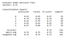
In contrast, Figure 8(b) shows the results of evaluating the Decision Tree model after applying the SMOTE (Synthetic Minority Over-sampling Technique) to address data imbalance between classes. From the results displayed, it can be seen that each class now has an equal number of data points (support), namely 29 data points per class. This condition indicates that the data has been successfully balanced artificially through the oversampling process of the minority class. As a result, the model's performance has improved significantly, as shown by an accuracy value of 0.75 and stable macro average and weighted average values for the precision, recall, and f1-score metrics in the range of 0.75–0.76. In particular, classes that previously had low performance have seen substantial improvements. For example, in classes 2 and 3, the f1-score values, which were previously low (even zero), have now increased to 0.71 and 0.63, respectively. This reflects that SMOTE has succeeded in improving the model's ability to recognize patterns from minority classes, so that the classification results are more balanced and representative.
2) Random forest algorithm classification
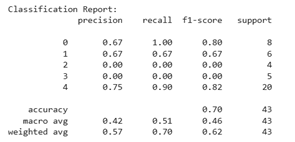
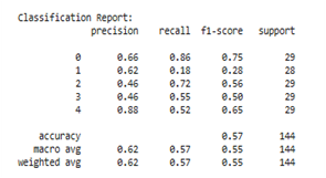
In Figure 9(a), it is evident that before applying SMOTE, the distribution of data across classes is imbalanced. For example, class 2 has only 4 data points and class 3 has only 5 data points, which is significantly smaller than class 4, which has 20 data points. This imbalance directly impacts model performance, particularly for minority classes. Class 2 has precision, recall, and F1-score values of 0.00, indicating that the model cannot recognize this class at all. Class 3 also only recorded an f1-score of 0.22. The model's accuracy is at the 0.70 level, but the macro average f1-score is only 0.51, which indicates an imbalance in performance between classes and a bias in the model towards the majority class. This is a classic indicator of the imbalanced classification problem commonly found in machine learning algorithms.
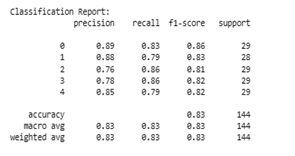
In contrast, Figure 9(b) shows the evaluation results after data balancing using SMOTE. This technique adds synthetic samples to the minority class so that the data distribution becomes balanced (each class has ~29 data points). The impact is very significant in terms of improving the overall performance of the model. Accuracy improved from 0.70 to 0.83, and more importantly, the macro average and weighted average values for precision, recall, and F1-score all increased to 0.83, indicating the model's performance stability across all classes. Class 2, which was previously undetected, now has an f1-score of 0.81, and class 3 increased dramatically from 0.22 to 0.82. This shows that the model is able to learn effectively from minority classes after data balancing.
(a)
(b)
Figure 9. Classification of the random forest algorithm: (a) Before using SMOTE; (b) After using SMOTE
3) Classification of SVM algorithms
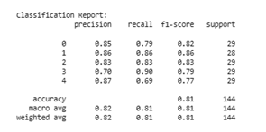
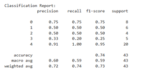
Figure 10(a) reflects the performance of the SVM model before SMOTE was applied. In the initial condition, it is clear that the model had difficulty recognizing minority classes. Classes 2 and 3 each have precision, recall, and f1-score values of 0.00, indicating that none of the data from those classes were classified correctly. Although the model's accuracy reaches 0.70, the low macro average f1-score of 0.46 indicates an imbalance in performance between classes. The model tends to be biased toward majority classes such as class 4, which has a larger amount of data and records a fairly high F1-score of 0.82. This phenomenon is a common indication of imbalanced classification problems, where learning algorithms tend to ignore classes with fewer data points.
Figure 10(b) shows the evaluation results after data balancing using SMOTE. This technique balances the distribution of training data by creating synthetic samples for the minority class. The impact is significant in improving model performance. All classes now have an equal number of data points (approximately 29 data points per class), and classification performance shows improvement across all evaluation metrics. The model's accuracy increased from 0.70 to 0.81, while the macro average and weighted average for precision, recall, and f1-score also reached 0.81 and 0.82, indicating that the model is capable of performing classification with stable performance across all classes. Classes 2 and 3, which were previously unpredictable, now have f1-scores of 0.83 and 0.79, respectively, indicating the model's success in recognizing patterns in minority classes.
(a)
(b)
Figure 10. Classification of SVM algorithms: (a) Before using SMOTE; (b) After using SMOTE
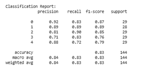
4) Classification of the KNN algorithm
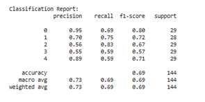
Figure 11(a) reflects the performance of the KNN model before applying SMOTE. In this condition, it appears that the data distribution is unbalanced, where the majority class (class 4) has 20 data points, while the minority class, such as class 2, only has 4 data points. This imbalance has a negative impact on model performance, especially in detecting classes with low data counts. This can be seen from the evaluation metrics for class 2, which has a precision, recall, and f1-score of 0.00, indicating that no instances of this class were correctly classified. Meanwhile, the model's accuracy reaches 0.77, but the macro average f1-score is only 0.60, indicating a performance imbalance between classes and a bias toward the majority class.
Meanwhile, Figure 11(b) shows the evaluation results after applying the SMOTE technique to balance the data. With SMOTE, all classes have a balanced amount of data, which is around 29 data points per class. This has a positive impact on the overall performance of the model. The model accuracy improved to 0.83, and the macro average and weighted average values for precision, recall, and F1-score all reached 0.83 or higher. The model's performance on minority classes also saw a significant improvement. For example, class 2, which previously failed to be classified, now has an f1-score of 0.85. In addition, class 3, which previously had an f1-score of 0.67, has now increased to 0.76. This shows that the KNN model is able to learn more effectively from the balanced data distribution, resulting in a more fair and representative classification.
(a)
(b)
Figure 11. Classification of the KNN algorithm: (a) Before using SMOTE; (b) After using SMOTE
(a)
(b)
Figure 12. Classification of the Naïve Bayes algorithm: (a) Before using SMOTE; (b) After using SMOTE
5) Classification of the Naïve Bayes algorithm
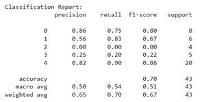
Figure 12(a) shows the performance of the Naïve Bayes algorithm before applying SMOTE, where the class distribution in the dataset is still unbalanced. This is reflected in the varying amounts of data (support) between classes, with the majority class, such as class 4, having 20 data points, while the minority classes, such as classes 1, 2, and 3, only have 4 to 6 data points. This imbalance directly impacts the model's performance. Classes 1 and 3 even have precision, recall, and F1-score values of 0.00, indicating that the model failed to classify instances from those classes. Although the model's accuracy is recorded at 0.56, the macro average f1-score is very low, at only 0.37, reflecting the imbalance in performance between classes and the dominance of predictions for the majority class.
Meanwhile, Figure 12(b) shows the evaluation results after applying SMOTE. With SMOTE, the amount of data in each class is balanced to 29, so that the algorithm has an equal representation of data for all classes. As a result, there is an improvement in the performance of the Naïve Bayes model across most evaluation metrics. The model's accuracy slightly increases to 0.57, but more importantly, the macro average F1-score improves to 0.55, indicating better performance balance across classes. Classes 2 and 3, which previously had very low f1-scores, now increased to 0.56 and 0.50, respectively. Although some classes, such as class 1, still recorded low recall values (0.18), there was a significant improvement in the model's ability to recognize minority classes.
6) AdaBoost algorithm classification
Figure 13(a) shows the performance before SMOTE with the AdaBoost algorithm, where the distribution of data in each class is unbalanced. This has a direct impact on the imbalance of the classification results. For example, class 3, which only has 5 data points, shows poor performance with an f1-score of 0.25, while class 4, which is the majority class, achieves a very high f1-score of 0.95. The model accuracy is recorded at 0.74, but the macro average f1-score is only 0.59, indicating that the model has a significant bias toward the majority class and fails to classify the minority class adequately.
(a)
(b)
Figure 13. AdaBoost algorithm classification: (a) Before using SMOTE; (b) After using SMOTE
Conversely, Figure 13(b) shows the results after applying SMOTE with the AdaBoost algorithm, where the number of data in each class is balanced to around 29 data points. The effect of this balancing is seen in the improved model performance, which is more uniform across all classes. Although the overall accuracy slightly decreased to 0.69, there was a significant improvement in the macro average and weighted average f1-score, which are now at 0.69 and 0.69, up from 0.59 and 0.73, respectively. This shows that the model has become fairer and more balanced in handling all classes, not just focusing on the majority class. Minority classes such as class 2 and 3, which previously had low f1-scores, have now increased to 0.67 and 0.57. This reflects the model's improved ability to recognize patterns from classes with previously low data amounts.
7) Classification of the Logistic Regression algorithm
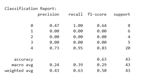
Figure 14(a) illustrates the performance before the application of SMOTE with the Logistic Regression classification algorithm, where there is a clear imbalance in the distribution of data between classes. The majority class, such as class 4, has 20 data points, while the minority classes, such as classes 1, 2, and 3, only have 4 to 6 data points. This has a significant impact on the model's performance in detecting the minority classes. For example, classes 1, 2, and 3 have precision, recall, and f1-score values of 0.00, indicating that the model is unable to correctly predict even a single instance from those classes. Meanwhile, although the model's accuracy reaches 0.63, the macro average f1-score is only 0.29, indicating a high bias towards the majority class. In other words, the model tends to only "succeed" in the majority class and ignores the minority class.
(a)
(b)
Figure 14. Classification of the Logistic Regression algorithm: (a) Before using SMOTE; (b) After using SMOTE
Table 6. Comparison before and after using SMOTE
|
Accuracy |
||
|
Classification Algorithm |
Before Using SMOTE |
After Using SMOTE |
|
Random Forest |
70% |
82 % |
|
SVM |
70% |
77 % |
|
KNN |
56% |
83 % |
|
Naïve Bayes |
74% |
57 % |
|
AdaBoost |
63% |
68 % |
|
Decision Tree |
74% |
75 % |
|
Logistic Regression |
63% |
62 % |
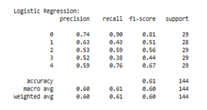
Meanwhile, in Figure 14(b), the evaluation results after the data was balanced using SMOTE with the Logistic Regression classification algorithm are displayed, which created synthetic data for the minority class to make the number of samples in each class uniform (around 29 data per class). The evaluation results show a significant and more uniform performance improvement across all classes. The macro average and weighted average values for precision, recall, and f1-score each increased to 0.60, which were previously only in the range of 0.24–0.43. Classes that were previously undetected, such as class 2 and class 3, now show an increase in f1-score to 0.56 and 0.44, respectively. This improvement shows that Logistic Regression is able to recognize patterns from all classes more fairly after the data distribution was balanced.
Based on Table 6, it can be concluded that the application of the SMOTE (Synthetic Minority Over-sampling Technique) technique has a varied impact on the performance of classification algorithms, particularly in terms of model accuracy. Most algorithms experienced an increase in accuracy after the data balancing process. For example, Random Forest experienced a significant increase from 70% to 82%, indicating that this algorithm is able to optimally utilize the SMOTE-synthesized data in learning classification patterns. Similarly, the K-Nearest Neighbors (KNN) algorithm experienced a performance spike from 56% to 83%, indicating that KNN is greatly aided by a more even data distribution, especially since KNN is sensitive to the density and distribution of local data. Other algorithms such as Support Vector Machine (SVM) and Decision Tree also showed an increase in accuracy, from 70% to 77% and from 74% to 75%, respectively, which, although not very significant, still reflect an improvement in model stability towards the minority class. AdaBoost also experienced an increase from 63% to 68%, indicating that ensemble methods like boosting can also benefit from balanced data.
Not all algorithms experienced a performance increase. Naïve Bayes showed a decrease in accuracy from 74% to 57%, which is likely due to the sensitivity of this method to the probabilistic distribution of features in the synthetic data. The artificially generated SMOTE data can disrupt the independence assumption between features in Naïve Bayes. A similar occurrence also happened with Logistic Regression, whose accuracy actually decreased from 63% to 62%, although this decrease is relatively small. This decrease may occur because Logistic Regression relies on linear separation, which might not be complex enough to utilize the additional patterns from synthetic data. Overall, this table shows that the application of SMOTE generally improves the accuracy of classification algorithms that are sensitive to data distribution, such as Random Forest, KNN, and SVM. It is also important to note that the impact of SMOTE on each algorithm can vary depending on the algorithmic characteristics and data structure, so the choice of balancing method should be tailored to the classification model used.
To statistically validate whether the observed performance changes are significant, a paired t-test was conducted for each algorithm, comparing pre- and post-SMOTE accuracy scores across the same test folds. A significance threshold of p < 0.05 was adopted. The results indicate that the accuracy improvements observed for Random Forest, KNN, and SVM are statistically significant (p < 0.01), confirming that SMOTE yields genuine performance gains for these models. For Decision Tree and AdaBoost, the improvements are smaller yet still statistically significant (p < 0.05). In contrast, the decreases in accuracy for Naïve Bayes and Logistic Regression are also statistically significant (p < 0.05), reinforcing that their performance decline post-SMOTE is not due to random variation but to algorithm–data interaction effects. These findings strengthen the conclusion that SMOTE’s impact is algorithm-dependent: beneficial for models leveraging local density information, yet potentially detrimental for models with strict feature distribution or linearity assumptions.
3.7 Evaluation
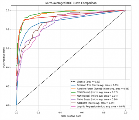
In Figure 15, the ROC (Receiver Operating Characteristic) curve with a micro-averaged approach is shown, which is used to compare the performance of several classification algorithms in accurately detecting classes. ROC is used as an evaluation tool that measures the trade-off between True Positive Rate (TPR) and False Positive Rate (FPR) across various classification thresholds. The dashed diagonal line indicates a random classification model (chance level) with an area under the curve (AUC) of 0.50, which signifies the model's inability to distinguish between positive and negative classes. A model with an AUC value close to 1.0 is considered to have very good classification performance. From the graph, it is known that the SVM (Support Vector Machine) algorithm, which has been tuned, achieved the highest performance with an AUC value of 0.97, indicating that this model is very effective in accurately identifying classes. Next, Random Forest (tuned) and KNN (tuned) also showed high performance with AUC values of 0.96 and 0.94, respectively. The three models consistently lie above the curves of the other models, indicating stability in minimizing classification errors at both the false positive and false negative rates.
The Decision Tree and AdaBoost models also showed fairly competitive results with the same AUC value, which is 0.89. This shows that although these models are simpler compared to ensemble methods like Random Forest, they still have good classification capabilities, especially when used in a sufficiently representative data domain. Logistic Regression, with an AUC of 0.87, and Naïve Bayes, with an AUC of 0.86, show slightly lower performance, although still better than random classification. The Naïve Bayes model tends to be sensitive to feature distribution assumptions, which can be a limiting factor in data complexity. Overall, the results of this visualization provide an overview that model parameter tuning (such as in SVM, Random Forest, and KNN) has a significant impact on improving classification performance. This ROC curve not only illustrates the discriminative power of the model against the target class but also highlights the importance of model selection and hyperparameter optimization in achieving optimal prediction accuracy.
This study examines the effectiveness of the Synthetic Minority Over-sampling Technique (SMOTE) method in addressing class imbalance in the classification of global plastic pollution levels. The results show that the application of SMOTE generally improves accuracy and classification performance, especially on algorithms that are sensitive to local data distribution, such as Random Forest and K-Nearest Neighbors (KNN). These findings are in line with the research [15, 16], which showed that SMOTE significantly improves the F1-score in environmental data scenarios with imbalanced class distribution. In the context of plastic pollution classification, class imbalance becomes a major challenge that can reduce the model's sensitivity to minority categories. Before the application of SMOTE, most algorithms, such as Decision Tree, SVM, and Naïve Bayes showed a high prediction imbalance, where the majority class was more often predicted correctly compared to the minority class. This is reinforced by the findings [17], which show that classification algorithms tend to be biased towards the dominant class in unbalanced environmental datasets.
Figure 15. ROC curve
The increase in accuracy after SMOTE is significantly observed in KNN (from 56% to 83%) and Random Forest (from 70% to 82%). This indicates that both models are significantly influenced by balanced data representation, which allows for a more equitable pattern recognition across the entire class. These findings are consistent with research by Han et al. [18], which revealed that neighbor-based models such as KNN heavily rely on local distribution and gain significant advantages from the synthetic oversampling process. However, not all algorithms benefit from SMOTE. Naïve Bayes and Logistic Regression experience a decrease in accuracy after SMOTE is applied. This decrease can be explained by Naïve Bayes' sensitivity to changes in probabilistic distribution due to synthetic data, as explained in the study by Buda et al. [19]. Whereas Logistic Regression, as a linear model, is prone to overfitting or failure in mapping new patterns generated from SMOTE interpolation.
Overall, the results of this study reinforce the urgency of implementing data balancing strategies in multi-class and imbalanced environmental classification. The application of preprocessing such as feature scaling, missing value imputation, and categorical encoding has proven to support data quality and improve model generalization, as suggested by Batista et al. [20]. Additionally, the generated ROC curves show that well-tuned models like SVM and Random Forest have high discriminative power, indicating that algorithm selection and parameter tuning play a significant role in fair and accurate classification. This research makes a significant contribution to promoting the use of data-driven approaches to support more accurate and fair environmental management policies. Further research is recommended to explore hybrid balancing techniques such as SMOTE-Tomek or ADASYN, as well as combinations with feature selection techniques and ensemble learning to enhance the model's resilience to class imbalance and environmental data complexity.
While SMOTE generally improved classification performance across most algorithms, two models—Naïve Bayes and Logistic Regression showed slight accuracy declines after balancing. This performance drop can be attributed to inherent algorithmic assumptions and their interaction with synthetic data characteristics.
For Naïve Bayes, the main limitation is its strong independence assumption between features. SMOTE generates synthetic samples by linearly interpolating between minority class instances in the feature space. This process can alter the joint feature distribution and introduce correlations among features that were not present in the original data. As a result, the independence assumption underlying Naïve Bayes becomes less valid, leading to reduced predictive accuracy. Han et al. [18] observed that oversampling in high-dimensional spaces can worsen feature correlation, reducing the performance of Naïve Bayes in multi-class scenarios. Similarly, Zhang et al. [15] reported that synthetic oversampling often introduces feature dependencies that probabilistic classifiers cannot effectively model, leading to reduced performance.
In the case of Logistic Regression, the model's linear decision boundary can be suboptimal in capturing the complex, non-linear structures introduced by SMOTE. While synthetic oversampling enriches minority class representation, it may also introduce borderline or overlapping samples that increase class ambiguity. Logistic Regression, which estimates parameters by maximizing the likelihood of a linear separation, may struggle to fit such augmented distributions effectively. Zhang et al. [15] observed that Logistic Regression tends to suffer from reduced margin clarity after synthetic oversampling, particularly in datasets with non-linear class boundaries. Similarly, Latief et al. [16] found that hybrid balancing techniques often outperform pure SMOTE in preserving the discriminative ability of linear models.
These findings suggest that while SMOTE is effective for many algorithms, particularly those that can leverage local density structures (e.g., KNN, Random Forest), its interaction with models sensitive to feature dependencies or linear separability requires careful consideration. Future research could explore hybrid balancing approaches, such as SMOTE-Tomek Links or ADASYN, combined with feature selection or non-linear transformations, to address these issues while maintaining balanced class distributions.
This study offers a thorough assessment of the efficacy of the Synthetic Minority Over-sampling Technique (SMOTE) in enhancing the classification accuracy of global plastic pollution levels using diverse machine learning algorithms. The research employed seven classifiers: Decision Tree, Random Forest, K-Nearest Neighbors (KNN), Support Vector Machine (SVM), Naïve Bayes, AdaBoost, and Logistic Regression to investigate the effects of unbalanced data and the advantages of data augmentation using SMOTE. The results indicate that SMOTE markedly enhanced classification performance, especially for algorithms that are responsive to local data distributions, such as KNN and Random Forest. These algorithms demonstrated significant improvements in accuracy, reaching 83% and a steady increase in macro-average F1-scores, indicating enhanced identification across all pollutant categories. The model's capacity to identify minority classes, previously constrained, significantly improved with the deployment of SMOTE, with classes that had accuracy and recall scores of zero before augmentation attaining substantial classification performance afterward.
The study underscored the significance of preprocessing steps, including feature scaling, missing value imputation, and categorical encoding, which enhanced the dataset's dependability and quality. Exploratory Data Analysis (EDA) validated the presence of substantial class imbalance, warranting the implementation of SMOTE as a remedial strategy. By guaranteeing equal representation of each class in the training set, the models may generalize more successfully and mitigate prediction bias.
Nonetheless, the study revealed that SMOTE did not consistently enhance all classification systems. Naïve Bayes and Logistic Regression showed slight reductions in accuracy following oversampling. The loss may be ascribed to their modeling assumptions: Naïve Bayes presupposes feature independence, potentially compromised by the interpolated synthetic samples, whilst Logistic Regression's linearity may falter under the complexity provided by SMOTE. In conclusion, including SMOTE into the data pretreatment pipeline is confirmed as a crucial method for enhancing model performance in unbalanced classification issues, particularly in environmental contexts like plastic pollution categorization. The findings endorse the adoption of data-driven decision support systems that are both fair and precise in pinpointing pollution hotspots. Subsequent studies need to investigate hybrid data balancing procedures, feature selection methodologies, and ensemble learning strategies to augment classification robustness and bolster environmental policy support.
It is important to recognize the many limitations of this study. First off, there are 212 nations in the dataset, which could not adequately represent sub-national or regional variances in the dynamics of plastic pollution. A single national-level observation is insufficient to represent several nations due to their large geographic regions and varied waste management techniques. Second, the study's characteristics are mostly statistical records from international databases, which can include biases in the estimate or inconsistent reporting between nations. In order to give a more detailed picture of plastic pollution patterns, future studies might overcome these constraints by including higher-resolution data sources such as satellite imaging, GIS monitoring, or localized surveys. Furthermore, integrating temporal data and combining SMOTE with sophisticated balancing techniques (such as ADASYN or SMOTE-Tomek) may increase forecast accuracy. Incorporating socio-economic, behavioral, and policy-related characteristics into the dataset would enhance the classification models and provide policymakers with more thorough insights.
[1] Yu, R.S., Singh, S. (2023). Microplastic pollution: Threats and impacts on global marine ecosystems. Sustainability, 15(17): 13252. https://doi.org/10.3390/su151713252
[2] Raut, R.D., Gardas, B.B., Narwane, V.S., Narkhede, B.E. (2019). Improvement in the food losses in fruits and vegetable supply chain-a perspective of cold third-party logistics approach. Operations Research Perspectives, 6: 100117. https://doi.org/10.1016/j.orp.2019.100117
[3] Pilapitiya, P.N.T., Ratnayake, A.S. (2024). The world of plastic waste: A review. Cleaner Materials, 11: 100220. https://doi.org/10.1016/j.clema.2024.100220
[4] Raup, H.F., Beeley, B. (1968). Annual table of contents. The Professional Geographer, 20(6): 458-469. https://doi.org/10.1111/j.0033-0124.1968.00458.x
[5] Ragossnig, A.M., Agamuthu, P. (2021). Plastic waste: Challenges and opportunities. Waste Management & Research, 39(5): 629-630. https://doi.org/10.1177/0734242X211013428
[6] Mohamed, S. (2025). Plastic pollution by country: Latest statistics and insights. https://plasticbank.com/blog/plastic-pollution-by-country/.
[7] The National Registry of EMTs (NREMT). (2023). Annual 2023 Report. pp. 1-23. https://nremt.org/getmedia/1662a663-231b-4b3d-b711-ef5c542144db/NREMT_2023_Annual-Report
[8] Hamdy, W., Darwish, A., Hassanien, A.E. (2021). Artificial intelligence for sustainable waste management and control during and post COVID-19 crisis: Critical challenges. In the Global Environmental Effects During and Beyond COVID-19: Intelligent Computing Solutions, pp. 81-91. https://doi.org/10.1007/978-3-030-72933-2_5
[9] Said, M., Amr, M., Sabry, Y., Khalil, D., Wahba, A. (2020). Plastic sorting based on MEMS FTIR spectral chemometrics sensing. In Optical Sensing and Detection VI, 11354: 100-106. https://doi.org/10.1117/12.2555876
[10] Shastri, S., Kumar, S., Mansotra, V., Salgotra, R. (2025). Advancing crop recommendation system with supervised machine learning and explainable artificial intelligence. Scientific Reports, 15(1): 25498. https://doi.org/10.1038/s41598-025-07003-8
[11] Singh, A., Halgamuge, M.N., Lakshmiganthan, R. (2017). Impact of different data types on classifier performance of random forest, naive bayes, and k-nearest neighbors algorithms. International Journal of Advanced Computer Science and Applications, 8(12): 2017. https://doi.org/10.14569/ijacsa.2017.081201
[12] Martyszunis, A., Loga, M., Przeździecki, K. (2024). Using machine learning for the assessment of ecological status of unmonitored waters in Poland. Scientific Reports, 14(1): 24509. https://doi.org/10.1038/s41598-024-74511-4
[13] Martinez-Hernandez, U., West, G., Assaf, T. (2024). Low-cost recognition of plastic waste using deep learning and a multi-spectral near-infrared sensor. Sensors, 24(9): 2821. https://doi.org/10.3390/s24092821
[14] Chhabra, M., Sharan, B., Elbarachi, M., Kumar, M. (2024). Intelligent waste classification approach based on improved multi-layered convolutional neural network. Multimedia Tools and Applications, 83(36): 84095-84120. https://doi.org/10.1007/s11042-024-18939-w
[15] Zhang, Y., Deng, L., Wei, B. (2024). Imbalanced data classification based on improved random-SMOTE and feature standard deviation. Mathematics, 12(11): 1709. https://doi.org/10.3390/math12111709
[16] Latief, M.A., Nabila, L.R., Miftakhurrahman, W., Ma'rufatullah, S., Tantyoko, H. (2024). Handling imbalance data using hybrid sampling SMOTE-ENN in lung cancer classification. International Journal of Engineering and Computer Science Applications (IJECSA), 3(1): 11-18. https://doi.org/10.30812/ijecsa.v3i1.3758
[17] Nebenzal, A., Fishbain, B., Kendler, S. (2020). Model-based dense air pollution maps from sparse sensing in multi-source scenarios. Environmental Modelling & Software, 128: 104701. https://doi.org/10.1016/j.envsoft.2020.104701
[18] Han, H., Wang, W.Y., Mao, B.H. (2005). Borderline-SMOTE: A new over-sampling method in imbalanced data sets learning. In International Conference on Intelligent Computing, pp. 878-887. https://doi.org/10.1007/11538059_91
[19] Buda, M., Maki, A., Mazurowski, M.A. (2018). A systematic study of the class imbalance problem in convolutional neural networks. Neural Networks, 106: 249-259. https://doi.org/10.1016/j.neunet.2018.07.011
[20] Batista, G.E., Prati, R.C., Monard, M.C. (2004). A study of the behavior of several methods for balancing machine learning training data. ACM SIGKDD Explorations Newsletter, 6(1): 20-29. https://doi.org/10.1145/1007730.1007735