V. Vijayaraj*![]() | M. Balamurugan
| M. Balamurugan![]() | Monisha Oberoi
| Monisha Oberoi![]()
© 2025 The authors. This article is published by IIETA and is licensed under the CC BY 4.0 license (http://creativecommons.org/licenses/by/4.0/).
OPEN ACCESS
Big data processing is crucial for extracting insights from large datasets, involving storage, cleansing, organization, modeling, analysis, and presentation. However, many face challenges with complex data systems, long provisioning times, and redundant boot disks. Containers, like Docker, address these issues by allowing distributed applications to run without full virtual machines. Despite this, Docker’s Swarmkit struggles with heterogeneity in clusters, where nodes vary in resource types and availability. To address this, we propose a resource-aware placement technique for heterogeneous Docker container clusters, using a Modified Log-Structured Merge (MLSM) data structure. This combines Cuckoo and Bloom Filters to efficiently distribute resources and maintain filter synchronization, providing better space utilization. Experimental results show that MLSM outperforms current methods in terms of performance and efficiency.
big data processing; docker swarm optimization; modified log-structured merge; bloom filters; cuckoo filters; data processing
1.1 Background of big data processing and docker importance
Big data refers to information assets that have high velocity, variety, and/or volume and cannot be processed using conventional IT infrastructure and methods [1]. Large companies and organisations used to be the only ones that needed it, but now even average people are seeking out big data processing choices to handle the mountains of data that their old IT systems just can't handle [2]. Problems that regular people face include the need for and supply of a sophisticated data processing system, the connection of complicated big data analytics, and the exertion in using these tools. This is why companies need a data processing system that is simple to build and create, inexpensive, and easy for users to use [3].
When it comes to big data analysis, the best and most well-established infrastructure is cloud-based big data processing solutions. To optimise performance, get the finest services, and lessen the danger of being dependent on any one provider, most enterprises and customers are now moving towards multi-cloud infrastructure [4]. The majority of cloud-based systems are built on virtualization, which is a critical technology of cloud computing. Many kinds of big data analytics aren't appealing to regular users because of the complicated migration process, challenges with load balancing and deployment, and the demand of large and redundant resources [5]. The aforementioned issues with big data analysis for regular people may be amenable to the container-based virtualization technology Docker's new Swarm for the creation of different kinds of multicloud distributed systems [6, 7]. Unfortunately, the data processing component of this container-based knowledge receives less attention than Docker, which is mostly employed in the software development business.
The suggested edge cloud design [8] makes use of Big Data processing technologies like Apache Spark and Hadoop Cluster, which, although shrunk to fit the constraints of IoT devices, nonetheless provide great speed, variety, and volume. The system is built on top of Docker, a containerisation technology that facilitates service coordination inside a device cluster. In order to evaluate the organisation's efficiency in relation to the limitations of the Raspberry Pi, data is collected using a cluster-based measurement and reporting tool and a Prometheus-based monitoring stack [9]. There has been an incredible deluge of data made available online in the last several decades. Numerous services, including websites, mobile apps, and online games, are utilised by hundreds of thousands of individuals who access the Internet. On the back end, the service providers rely on cutting-edge cloud infrastructures like Microsoft Azure and Amazon Web Service [10, 11]. Data centres and cloud environments utilise virtualization, an emerging technology that focuses on offering services at scale, to enhance hardware besides expansion efficiency.
The virtual machine is a popular approach to system-level virtualization that separates various system resources [12]. But, on a large-scale system, users would likely be running several copies of the same operating system and many redundant boot discs if services were provided through virtual machines [13]. Virtualization of containers is old news now; big data processing platforms use containers as its foundational computing unit [14], and Unix-like operating systems used them for more than a decade. On the other hand, Docker and other emerging containerisation systems become standard fare for creating applications. Docker simplifies the tooling necessary to construct and manage containers by building on previously existing open-source technologies (e.g., cgroup). Containers on a physical computer are basically simply ordinary processes running in the background, but when viewed from the system perspective, they have access to a virtualized situation that includes not just CPU and memory but also disc I/O, and more [15].
On physical devices, we launch Docker containers using the "Docker run image" command. Along with the desired disc image, users have the opportunity to specify other parameters, such "-m" and "-c", to restrict a container's resource access [16]. Resource contention occurs among containers on every host computer, even though options set a maximum quantity. First thing a cluster should do when it gets "Docker run" orders from clients is choose a physical machine to run the containers. Using a bin-pack method, the default container placement scheme, Spread, attempts to allocate a container to the node that has the fewest operating containers [17]. Spread does not include two key features of the system, even though it intends to distribute jobs evenly among all nodes. To begin, there is no hard and fast rule that says all of the nodes in a cluster must be similar. Many different kinds of nodes, each with its own unique set of capabilities and resources, are often found in a cluster. For instance, compared to a generic desktop, a state-of-the-art server can easily handle more tasks running in parallel [18]. The dependency matrix is a revolutionary approach introduced by cloud computing that eliminates the need for programmes to deal with hardware dependencies, operating system specifications, and possible library conflicts in traditional deployment settings [19, 20]. Docker containers are widely used for distributed applications, but Docker's Swarmkit faces challenges in managing heterogeneous clusters, where nodes differ in resource types and availability. This heterogeneity complicates resource allocation, as services may have varying demands, such as CPU-intensive or memory-intensive requirements. In this research, we address these limitations by proposing a resource-aware placement technique for Docker container clusters. We introduce a Modified Log-Structured Merge (MLSM) scheme, utilizing Cuckoo and Bloom Filters to efficiently distribute resources across nodes. The MLSM method ensures optimal resource utilization, syncing filters with keys of all Sorted String Tables (SSTables) while minimizing space usage. Experimental results demonstrate that MLSM outperforms current methods, offering superior performance and efficiency in heterogeneous cluster environments.
Software applications were usually delivered on bare metal servers or virtual machines before Docker and containerisation came along. Docker, an open-source technology, changed everything by letting users build and deploy apps with ease by packaging them with their dependencies into containers. Containerisation, made possible by Docker, ensures that programmes may run efficiently and without errors across various computing environments by enclosing all required dependencies, such as frameworks and libraries [21]. One major perk of Docker containers is how lightweight they are. This makes them perfect for transferring and running in many computing settings, regardless of the operating system or configurations used by the host.
1.2 Motivation of the work
Application deployment used to be a laborious, resource-intensive manual operation until container technologies came around. The deployment process was much improved and streamlined with the advent of container technologies, especially Kubernetes and Docker. Currently, there are a number of options available for load balancing containerised applications, each designed for a certain use scenario. With Docker's integrated capabilities for load balancing and service discovery, scaling has become much easier.
Developers may now devote more effort to actually making their apps and less time to developing these ancillary tasks. Docker reduces the time it takes to deploy highly available and scalable applications by automating operations like configuring DNS for service discovery and adding apps to the load balancer pool when scaling is needed. These developments have not eliminated efficiency issues with current approaches, and new algorithms lack the scalability necessary for broad use. The growing use of containers has made load balancing a must-have feature, calling for more investigation into effective ways to handle it.
1.3 Contribution of the research work
A novel container placement technique is suggested in this project's investigation. Instead of using the default spread scheme, the suggested approach distributes containers according to the resources available in a diverse cluster and the changing needs of different types of containers. The model begins by tracking containers that provide a service in order to determine the most common resource type for that service. In order to minimise imbalanced resource utilisation on the nodes, it then assigns containers with complimentary demands to the same machine. When a particular resource reaches its limit, the system will move containers that use a lot of that resource to other nodes. In this research, two large data probabilistic data structures—the cuckoo filters and the modified bloom filters—are examined. An LSM tree is used to evaluate the efficacy of these two probabilistic data structures. The conventional wisdom is that using bloom filters to improve query speed is the way to go. However, cuckoo filters offer the ability to exclude unwanted elements, so we opted for them instead. It follows that cuckoo filters should outperform bloom filters in compaction and merging operations.
1.4 Paper organization
The background of big data processing, docker swarm optimization, motivation and contribution of the research work is mentioned in Section 1.
The brief explanation of the related work with its drawback is mentioned in Section 2.
The theoretical docker swarm with block diagram is explained in Section 3, where problem formulation is mentioned in Section 4.
The explanation of proposed methodology with neat explanation is given in Section 5, the implementation of docker swarm in virtualization is given in Section 6.
The results analysis and its discussion is given in Section 7, where the conclusion of the research work is shown in Section 8.
A work scheduling technique based on multi-objective hybrid optimisation has been introduced as BWUJS, or Black Widow Updated Jellyfish Search [21]. From a Bigdata point of view, this study examines task creation. Map Reduce, in conjunction with a K-means clustering model, clusters the jobs. Next, we estimate the priorities of the tasks once they have been clustered. In the end, priorities, makespan, completion time, resource utilisation, and imbalance are used to schedule tasks using BWJSU.
An exhaustive review of the classic K-means method [22] is the starting point for this study, which ultimately proposes an enhanced version of the technique. The experimental findings show that the suggested enhanced K-means algorithm works better than the original, with much better accuracy and fewer classification mistakes, reaching an error rate below one.
Using the outcomes of a deep reinforcement learning model's predictions, the grouping technique is adjusted before a data stream's frequency changes [23]. Because of this, the system will be able to efficiently manage its resources and respond swiftly to changes in data streams. For effective massive data streaming in cloud systems, Gaussian adapted Markov model (GAMM) is used [24]. An effective and error-free management of time-bound big data streaming applications is the goal of this effort. To conduct the fluctuation analysis, this work also makes use of the gating technique to identify the set of features necessary to produce the nonlinear distribution of data and the fat convergence solution.
A fog layer utilising a novel and enhanced geographic load-balancing method has been introduced [25]. In order to advance the user experience for augmented and virtual reality apps, it optimises the distribution of loads and supplies quality of service (QoS) characteristics. In virtual reality and augmented reality games that use electroencephalograms, the iFogSim toolbox provides experimental validation of the framework. Furthermore, a wide variety of situations are used to test the proposed framework.
The two algorithms: dynamic SDN (dSDN) then priority scheduling and congestion management (eSDN) are developed [26]. The tDQN agent iteratively learns to reduce network latency by improving decision-making for switch-controller mapping using a reward-punish mechanism. Our method, tDQN, optimises latency and dynamic flow mapping without adding more controllers at the best possible locations. In order to dynamically redirect traffic to the most appropriate controller, a multi-objective optimisation problem is developed for flow fluctuation. Throughput, latency, packet loss are among of the metrics where the tDQN excels, according to comprehensive simulation findings that account for a wide range of network conditions and traffic.
Adaptive and self-organizing behaviours are modelled after in bioinspired algorithms, which are utilised by Load Balance to dynamically distribute workloads among cloud resources [27]. Using concepts from swarm intelligence and evolutionary algorithms, the proposed method iteratively enhances load distribution solutions. This optimisation method improves cloud load balancing and provides a sustainable solution for current cloud infrastructures by drawing inspiration from nature.
To improve traffic distribution within a certain geographic cluster, reinforcement learning [28] is used to optimise the relational parameters of neighbouring cells. The proposed method for accurate traffic flow prediction is the spatial-temporal- graph convolution neural network, or STECA-GCN. The Chaotic Horse Ride Optimisation Algorithm (CHROA) and big data analytics (BDA) is used [29]. By using chaotic method gives the Horse Ride Optimisation Algorithm (HROA) more optimisation power. Load balancing, AI-based optimisation of available energy resources, and evaluation using many metrics are all features of the suggested CHROA paradigm. The CHROA model achieves better outcomes than previous models, according to the experimental data.
A proposed efficient heterogeneous resource scheduling process based on the Hybrid Gradient Descent Golden Eagle Optimisation (HGDGEO) algorithm [30] is developed to deal with the problems that could arise when processing big data in the Hadoop heterogeneous cloud environment. The HGDGEO algorithm's simulation results demonstrated its superiority in comparison to other resource scheduling algorithms in terms of makespan, load balance, besides throughput.
3.1 Big data analysis
The goal of big data analysis is to help with decision-making, forecast, besides other forms of inferencing by mining and extracting significant patterns from large amounts of input data. In traditional data analysis, a small quantity of cleansed first-hand data is examined using conventional statistical approaches including factor, cluster, correlation, and regression analysis. In most cases, we only test a few of hypotheses that we formulate prior to data collection [31]. Big data analysis, on the other hand, may examine enormous amounts of unstructured and dirty data using either improved computational models or more conventional statistical approaches. When it comes to collecting, cleaning, modelling, and visually interpreting data, among other operations involved in big data investigation, a big data analytic is more of a system, platform, or framework than a singular tool or technology.
3.2 Docker container and docker swarm
To construct comparable to a virtual machine (VM) but does not use virtual hardware emulation, a method that is somewhat distinct from virtualization is known as containerisation or container-based virtualization. Although containers have been around for a long time in Unix and Linux, they are making a comeback in the business sector as a viable alternative to virtual machines (VMs). The creation of containers occurs in the user space, above the operating system kernel, so containerisation might be viewed as a virtualization at the OS level. It is possible to build several containers in different user areas on a single host, although they utilise far less resources compared to virtual machines.
Containerisation is exemplified by the Docker container. Using Docker, a container-based technology, application development, deployment, and execution can be done easily and automatically. As seen in 0 1 [32], Docker Engine allows for the creation of isolated environments, or containers, that are comparable to virtual machines (VMs) but lack their own operating system (OS). As a result, all containers share the same OS kernel. In contrast, a container contains the executable and any necessary library files to launch a programme. On Linux, the operating system itself serves as the Docker Host, while on non-Linux machines, a separate installation of the Docker Host is required [32]. In comparison to the real virtual machine (VM), this Docker host uses very less resources. This Docker Host is known as the default by Docker as it is pre-installed and needed to operate the Docker Engine.
Figure 1. Docker containers on linux host [32]
With Docker Swarm, an orchestration and cluster organization tool, several Docker nodes may be linked and managed as one virtual system. As an improvement on Docker container technology, it allows for the creation of distributed systems that may be deployed across many clouds. It improves upon conventional container technology and makes the container-based system trustworthy by adding capabilities like scalability, security, dependability, maintainability, and availability to the Swarm cluster.
The goal of the suggested scheduler is to maximise the use of each worker node's resources by optimising container placement. Assumed throughout this article are the various resources—memory, CPU, bandwidth, and I/O—that a container needs to perform its services. The resource needs of a container also display temporal dynamism due to the fact that the services and workloads contained within it are subject to change. Therefore, we formulate the resource necessities of time. Mean $r_i^k(t)$ as the kth reserve obligation of the ith ampule at time t. Let $x_{i, i}=\{0,1\}$ be the container placement indicator. If $x_{i, i}=1$, is located in the j th node. Signify $W_i^k$ as kth node. Let $\mathcal{C}, \mathcal{N}, \mathcal{K}$ be the set of containers, work nodes, and the capitals, correspondingly. The use ratio of the k reserve in the $j$ th work node can be spoken as
$u_j^k(t)=\frac{\sum_{i \in C} x_{i, j} r_i^k(t)}{W_j^k}$ (1)
Then, the use ratio of the jth work node is $\max _k K u_j^k(t)$. The highest resource utilization amongst all the work nodes can be recognized as
$\vartheta=\max _{j \in N} \max _{k \in N} u_j^k(t)$ (2)
Since our proposed scheduler is to exploit the obtainable resources in node, the future scheduling problematic can be expressed as
$\max _{x_{i, j}} v$ (3)
$\text{S.t} \sum_j x_{i, j}=1 ; \forall i \in C$ (4)
$x_{i, j}$: A binary container placement indicator. If $x_{i, j}=1$, it means container $i$ is placed on node $j$; otherwise, it is not.
$u_j^k(t) \leq 1, \forall k \in K, \forall j \in N$ (5)
The utilization of any resource on any worker node must not exceed the capacity of that resource (i.e., utilization should be less than or equal to 1):
Each container must be located in a single worker node according to the requirement in Eq. (4), and no worker resource can have a utilisation ratio greater than one according to the need in Eq. (5).
5.1 Initial container placement
The command "docker run" is used by clients to create a new container and utilise a SwarmKit cluster. Consequently, selecting a worker node to serve as the container's host is the cluster's primary responsibility. As mentioned in Section 3, the default technique for placing containers does not account for dynamic resource contention. This is due to the fact that SwarmKit's management features are lacking an instrument to track the present state of the available resource. Conversely, the issue is handled by the suggested model with the introduction of the Modified LSM-Tree model.
Running on managers, Procedure 1 assigns a task to a exact worker.
|
Algorithm 1. Container Placement on Administrators |
|
1: Maintains a known features service set {KS} 2: {Wcand}=All running Wid 3: Function SID 4: for wid∈{Wcand} do 5: if ! Filters(wid) then 6: Remove wid from {Wcand} 7: if SID∈{KS} then 8: SDOM=DOM(SID) 9: Sort Wcand according to rSDOM 10: Return wid with highest rSDOM 11: else 12: Sort Pi i= =0 q ri/m for wid ∈Wcand 13: Return wid with highest average available resource |
To start, every manager keeps track of dockers' traits, including memory, CPU, bandwidth, and block i/o consumption, in a known service set (line 1). All running workers make up the initial candidate worker pool (line 2). Whenever a new container beginning task happens, the method reduces the candidate work set, W_c, and (lines 3-6) using all the filters that the user has chosen. After that, it verifies on line 7 if the container is associated with a recognised service. If so, the dominating resource property of the container will be stored in the S_dom parameter (line 8). We think about memory, CPU, bandwidth, and block i/o in the approach we're proposing. After sorting the W_c and set by dominating resource attribute, the highest available resource in the S_dom type will be returned, as indicated by the W_id with the highest value (lines 9-10). The W_id with the average greatest obtainable resource will be selected (lines 11-13) if the service is not discovered in {KS}.
5.2 Data collection and analysis
In order to evaluate the architecture, we will utilise two applications. One app will represent data collection on a fraction of the nodes, while the other will be placed on an Apache Spark cluster to analyse the data. System performance metrics, such the time it takes to process certain data, may also be retrieved through the applications.
In order to acquire data, a Node.js app sends a PUT request to the HDFS API along with the data's content, simulating data collection; this causes a file to be created within a certain time frame. Only the last three nodes of the cluster are used to deploy the data gathering application using a Compose file. As a result of the trial, we have a collection of sample documents that the programme can read and modify online; this allows us to change the document's size or content without updating and redelivering the application.
Examine the information. In order to examine the data, a Python programme is employed. The application checks recently created files for each phrase and counts the number of times it appears per second. Using the Apache Spark engine's given sample application as a starting point, the software has undergone minimal changes.
For every phrase that appears, the method use the standard paradigm to produce a list of (Key, Charge) pairs of the form (Word, 1), as mentioned before. To get the total number of times each word appears, the Reduce step is applied to every group. A single function, Reduce by key, handles the remaining two phases. Pseudocode demonstrating the method with an example Map Reduce solution application is shown below.
|
$\begin{aligned} & \text { Count } \\ & :=\text { Lines.FlatMap(lambda(line)\{line.split('''')\}) } \\ & . \text { map(lambda(word)\{(word,1)\}). } \\ & \text { reduceByKey(lambda(Val,acc)\{Val } \\ & + \text { acc }\} \text { )counts.pprint() }\end{aligned}$ |
Use the spark submit command in the Spark CLI to distribute the application among the workers in the cluster after it has been sent among the master nod.
5.3 Monitoring
In order to facilitate system monitoring, a three-component monitoring stack based on Prometheus is installed on the cluster. Free and open-source, Prometheus is an alarm and monitoring system that provides many interfaces to other platforms and makes use of a time series database.
Technologies such as Docker, HAProxy, and the ELK stack (Elastic search, Log stash, and Kibana) are examples of this type. Furthermore, the stack incorporates many "exporters" that collect metrics and expose them for Prometheus to collect, in line with Prometheus' operational philosophy of data extraction from multiple services.
Data visualisation and analysis tool Grafana is well-liked. The web-based programme Grafana allows users to build dashboards for data tracking and analysis. This solution was selected for a use case that needed to follow Docker containers on many Linux systems since it required little configuration. This led to the use of an almost complete implementation for Raspberry Pis. A bespoke Compose file with Docker containers is utilised to deploy the stack to the Docker cluster. In the final configuration, one of the nodes gets Grafana and Prometheus installed, while each Raspberry Pi gets Advisor and Node exporters loaded.
5.3.1 Modified log-structure merge tree
One data structure that dynamically optimises memory and disc access for fast writing is the MLSM tree. The LSM tree typically reads, writes, and inserts data into memory using a tree-based indexing method such an AVL or Red-black tree. So, before flushing the data structure into disc, sorting done beforehand. Upon disc flushing, the data structure transforms into a sorted string table, or SSTable, a key-value sorted file. Every time a client requested an insert or delete, the indexing algorithm sorted the keys, therefore this file is flushed in a sorted state. On the other hand, the LSM tree's query performance is one of its drawbacks. With a sparse index for each SSTable on the disc, we can search for a certain key in Olog(n) time. On the other hand, since LSM trees are log-based, the disk's SSTables are automatically sorted in reverse chronological order. Thus, a temporal complexity of O(n) and undesirable client waiting time result from checking every file to locate the client-requested key in the data structure. Databases like Cassandra, HBase, Accumulo, and Google Big Table typically display the LSM tree. The lengthy key query period was, however, resolved by all of these databases by the use of a bloom filter, a probabilistic data structure.
5.3.2 Probabilistic data structures
Database query speed may be optimised with the use of probabilistic data structures, which are low-memory-cost bit arrays. Hyperloglog, cuckoo, bloom, and KD-tree filters are just a few examples of the many data structures available. When these data constructions are positioned strategically in high ingestion schemes, they can save expensive disc searches, which is a huge boon to the system. One simple way to drastically reduce an application's throughput from hundreds of thousands to a few thousand operations per second is to have it search up an element in a huge database on disc. The primary focus of this research is on set membership analysis using cuckoo and bloom filters. Due to the following similarities in construction, these two data structures are structurally similar: (1) both employ hash functions to produce indexes, and (2) both put keys into their slots. converting keys to bits to maximise memory consumption and reading speed was (2) (3) are based on probability since the false positive rate is a measure of the maximum allowed hash collision inside the keys. The study's probabilistic data structures are summarised in Table 1, along with their key distinctions.
Table 1. Bloom and cuckoo filter contrast
|
Filters |
Hash Number |
Operation List |
Time Complexity |
|
|
|
-Deletions |
|
|
Cuckoo Filter |
2 |
-Insertions |
O(1) |
|
|
|
-Confirmations |
|
|
Bloom Filter |
Optimal k |
-Insertions |
O(1) |
|
|
|
-Confirmations |
|
5.3.3 Bloom filters
To determine if an element is a member of a set, probabilistic data structures called bloom filters are employed. The possibility of false positives—a situation in which the real element is not in the set but the result indicates otherwise—makes this data structure probabilistic. The building blocks of a bloom filter are hash functions, bits, and an array of bits that start off as zeros. Only two procedures are supported by bloom filters:
While changing the relevant bits from zero to one, new items are added and hashed several times.
The element is probably part of the set if it has been hashed and all of its matching bit values are one. Because bloom filters do not produce false negatives, if this is not the case, then the element in question does not belong to the set.
Because they do not save keys on the array, bloom filters significantly improve performance for large-scale database look-ups and significantly reduce storage requirements. Having said that, the false positive rate of bloom filters is fixed. Giving the incorrect impression that an item is part of the set is therefore possible (with a probability greater than zero). In addition, once an object is put to a bloom filter, it cannot be removed. Consequently, the false positive rate rises in proportion to the number of data input. The suggested optimisation technique determines the ideal hash function sum k based on the bit array size and insertion sum, which in turn is determined by the amount of false positive rate acceptance and the length of the bit array, which is m bits.
$F P R=\left(1-\left(1-\frac{1}{m}\right)^{k n}\right)^k \approx\left(1-e^{-\frac{k n}{m}}\right)^k$ (6)
$g=\operatorname{In}(f)=k \operatorname{In}(1-p)=k \operatorname{In}\left(1-e^{-\frac{k n}{m}}\right)$ (7)
$Optimal$ $k=\frac{m}{n} CCRIMEIn(2)$ (8)
$Optimal$ $m=-CCRIME\frac{n {In}(F P R)}{{In}(s)^2}$ (9)
In Eq. (6) the false positive rate of bloom filters is designed. The likelihood of a bit being zero is $1-\frac{1}{m}$ with "m" standing for the filter's bit array size. A bloom filter, on the other hand, can accommodate anything from one to k hash functions and n items. Hence, the likelihood needs to be increased to "k" times "n". As a result, the "k" number of hash functions raises the chance of a non-zero bit to the level of the false positive probability. $\left(1-\left(1-\left(\frac{1}{m}\right)\right)^{k n}\right)^k$. The ideal "k" number of hash functions is determined using Eqs. (7) and (8). A logarithmic expression is created from Eq. (7) in order to compute its derivative. To get the best "k" number of hash function expression, as indicated by Eq. (8), one can only take the derivative of Eq. (7). The ideal size of a bloom filter's bit array is determined by Eq. (9). Therefore, the conversion of the variable "k" in Eq. (6) by the expression in Eq. (8) yields the ideal bit array size. The ideal bit array and insertion value that are covered below are found using the suggested CCRIME.
A. An overview of RIME
Su et al. [33] introduced RIME, an innovative and effective optimisation approach. The primary physical effect it mimics is the freezing of airborne, noncondensed water vapour upon contact with cold surfaces, such as branches or objects. First, rime ice generation; second, soft RIME search strategy; third, hard RIME puncture mechanism; and last, greedy selection mechanism for the best answer make up the four primary steps of the RIME algorithm. During the first phase of rime generation, the RIME algorithm treats every search agent in the population as an agent. The algorithm's starting population consists of all RIME agents combined. Eq. (10) is used to initialise each agent in the population inside a specific search space:
$R_i=B_{\min }+r_i \times\left(B_{\max }-B_{\min }\right)$ (10)
where, $R_i$ represents each search agent, $B_{\max }$ and $B_{\min }$ represent the boundaries, correspondingly, and $r_i$ is a pseudo-random sequence among [0, 1].
A key tenet of the soft RIME search technique is the idea that particles in the soft rime would trap and condense any free particles that approach it, altering the stability of the soft rime in the process. If there is a large enough gap between the particles and the soft rime particles, the latter will evade capture and remain free. Over time, the soft rime will gradually expand its coverage area and catch a higher probability of particles as it condenses and collects free particles. Environmental variables, however, will cause the soft rime's covering area to eventually reach a constant state rather than an infinite growth. The following is the precise mathematical model that was developed by modelling the rules of motion for free particles and soft rime:
$\begin{aligned} R_{i j}^{\text {new }}=R_{\text {best }, j}+R f\times\left(h \times\left(B_{\max (i, j)}-B_{\min (i, j)}\right)\right. \left.+B_{\min (i, j)}\right), r_2<E\end{aligned}$ (11)
$R f=r_1 \times \cos \theta \times \beta$ (12)
$\theta=\pi . \frac{t}{10 . T}$ (13)
$\beta=1-\left[\frac{w .\ t}{T}\right] / w$ (14)
$E=\sqrt{(t / T)}$ (15)
where, $R_{i j}^{n e w}$ is the site of the free moving besides $R_{b e s t, j}$ is the best RIME agent in the RIME population. $r_1$ has a value -1 and 1, chosen at random. As the algorithm iterates, cos q will change. b controls the convergence of the algorithm and reflects the ambient elements in rime. It changes as the programme iterates. The distance between free particles is represented by h, which is a randomly assigned value between 0 and 1. Here, t is the current iteration count and T is the maximum iteration limit of the method. The increment of w determines the step function's segment count; 5 is the default. The chance of capturing free particles is denoted by E. As the algorithm runs more iterations, it will vary and typically show an upward trend.
The hard rime puncture mechanism mostly mimics the way particles move in environments with greater winds; when particles move in the same direction of growth, a cross phenomena known as hard rime puncture is easily possible between them. Also, the frequency of hard rime punctures increases in direct proportion to the hard rime's growth. In order to avoid being stuck in local optima, rime agents can trade particles and update each other's positions using the hard rime puncture mechanism, which also improves the algorithm's convergence capabilities. The hard RIME puncture strategy's mathematical model looks like this:
$R_{i j}^{\text {new }}=R_{\text {best }, j}, r_3<F^{\text {normr }}\left(S_i\right)$ (16)
where, $R_{i j}^{n e w}$ is the $j$ th particle of the finest rime agent in the populace and $R_{\text {best } . i}$ new is the updated particle location. The fitness charge of the current agent is regularized to produce $F^{\text {normr }}\left(S_i\right)$, which characterizes the likelihood that rime puncture. A sum at random among [0,1] makes up $r_3$.
The horizontal crossing operation often requires the employment of two separate rime agents. The capacity for exploration is greatly enhanced and algorithm convergence is accelerated by the ability of separate agents to each other through the horizontal crossover search. Given that the parent agents $x_i$ and $x_j$ may be characterised by Eqs. (17) and (18), let's pretend that they undergo a horizontal crossover operation:
$\begin{aligned} M S_i^n= & \varepsilon_1 \times x_{i n}+\left(1-\varepsilon_1\right) \times x_{j n} \\ & +C_1 \times\left(x_{i n}-x_{j n}\right)\end{aligned}$ (17)
$\begin{aligned} M S_j^n= & \varepsilon_2 \times x_{j n}+\left(1-\varepsilon_2\right) \times x_{i n} \\ & +C_2 \times\left(x_{j n}-x_{i n}\right)\end{aligned}$ (18)
where, $\varepsilon_1$ and $\varepsilon_2$, which are random variables distributed uniformly throughout the interval [0,1], are used in the provided equation. Furthermore, both $c_1$ and $c_2$ follow a normal distribution on the range [-1,1]. For agents ith and jth, the nth dimension is denoted by $x_{i n}$ and $x_{j n}$, respectively. Through the horizontal crisscross $x_j$, the nth position vectors' offspring, represented by $M S_j^n$, are created.
Two discrete site vectors of agents in a population are manipulated via the vertical crossover operator, a computational method. While reducing the number of changes to the normally searched position vectors, this method may allow some position vectors that are limited to a local optimum to continue searching. Because some position vectors tend to stagnate in the later stages of exploration, ants often reach a local optimum. By utilising a vertical crisscross search approach, agents can learn position vectors from each other and improve their ability to avoid local optimums. Assuming agent i's mth and nth position vectors undergo the vertical crossover process as indicated in Eq. (19):
$M S_i^m=\varepsilon \times x_{i m}+(1-\varepsilon) \times x_{i n}$ (19)
where, $\varepsilon$ characterizes a random sum among [0,1] and $M S_i^m$ signifies the mth site vector of the offspring produced by crisscross operation among the mth agent nth site vectors of agent i.
No more study or analysis was carried out on the performance of RIME as its initial research just suggested an optimisation strategy by modelling the changing shape of rime. Additionally, this paper's benchmark function studies have shown that it has a significant advantage in convergence and still has plenty of space for development. Furthermore, our experimental results show that it outperforms the general traditional algorithms when it comes to discovering high-quality persons to solve real-world challenges, and this is in relation to the feature selection problem. This paper associated RIME with other similar algorithms from various perspectives in order to learn more about its performance and find ways to make it better. It found that RIME could still do better in terms of the quality of the solutions it found and that its search capabilities could use some work to prevent it from reaching local optima.
In light of the foregoing, this work concluded from its examination of horizontal and vertical cross-search methods that it may significantly boost algorithm performance; furthermore, other research has employed this technique to improve the efficiency of certain optimisation algorithms. Motivated by this, this study improved the original RIME by including horizontal and vertical crossover search algorithms to increase its search capabilities, improve the quality of the solutions obtained, and prevent it from falling into local optima throughout the search process. Following the hard RIME puncture mechanism, the horizontal and vertical crossover search techniques primarily take action in the enhancement phase. Through enhancing RIME's search skills, CCRIME is able to acquire better solutions and enhance its optimisation capabilities in real-world scenarios.
B. Cuckoo filters
Since its introduction in 2014, cuckoo filters—a type of probabilistic data structure—have found extensive use in many network applications. To determine if an element is "probably" or "definitely" part of a set, cuckoo filters are utilised, similar to bloom filters. Bit arrays, slots, and buckets make up cuckoo filters. The bird that lays its eggs in a different nest and then, after a chick emerges, plucks the other eggs or chicks out of the nest is called a cuckoo.
Because cuckoo filters only utilise two hash functions, whereas bloom filters employ k, cuckoo filters provide space and temporal complexity that is comparable to that of bloom filters but with less hashing cost. But the big perk of cuckoo filters is that they can remove objects from the membership set thanks to their two-dimensional and capabilities. This has the potential to enhance databases like HBase, which undergo continuous SS Table merging and compacting. A load parameter in a cuckoo filter indicates what fraction of the filter's slots are now in use.
Half of the buckets in a cuckoo filter are already in use when the load is 75 percent. On the other hand, studies have shown that cuckoo filters start producing more false negatives as the load factor increases. The system was able to avoid producing false negatives while verifying the presence of keys during our experiments with a load factor below 65%. The load factor must be considered in order to determine if resizing or other actions are necessary to manage the filters at level.
$I_1(x)=\operatorname{hash}(x)$ (20)
$I_2=I_1(x) \oplus$ hash $\left(x^{\prime}\right.$ sfingerprint $)$ (21)
Eqs. (20) and (21) determine the index of the buckets that will be used to enter the fingerprint. By inputting the key into a hash function, the first function determines the index of the first bucket. On the other hand, the second index is determined by first computing the fingerprint hash value and then performing an XOR operation on the index of bucket. A new cuckoo filter cannot be generated until the specified capacity is matched with indexes one and two.
5.4 Migrating a container
All workers in a Swarmkit cluster compete for the same resources. One component of the suggested paradigm, the container monitor, keeps track of how much power each worker's containers use. Additionally, the worker maintains self-tracking of available resources. It notifies managers with an alert message that specifies the kind of bottleneck and expensive container of that kind if it detects that a draining resource becomes a bottleneck. Managers are tasked for assigning containers to workers when they get alert messages and then killing them on those workers to free up resources.
Docker is a free and open-source software stage for Linux container virtualization. This programme requires a certain version of the Linux kernel—specifically, 3.10 or later—and employs operating system-level virtualization, as indicated before. Docker allows processes to be executed in a contained setting. Operating in Docker is like putting a process in a vacuum: all it sees are its own offspring. Even though it shares the same operating system as other processes, this one can't see anything outside of its own little bubble, including other processes, files, and the entire system. The process's container is the bare minimum of an environment in which it executes. The container serves as a standalone OS, complete with its own file system, network, and peripherals. By mounting specific folders and files, sharing a network, and opening required ports, the container can communicate with the host containers.
You can't make a docker container without images. The image serves as a blueprint, pre-installing the operating system and all required apps. Local storage or a dedicated public registry (dockerhub) can house images. The Dockerfile uses a specific syntax to declaratively describe the image template. What follows is a sample image template with Ubuntu installed and the OpenALPR software pre-loaded.
|
$FROM ubuntu: 16.04$ $RUN apt - get update$ $\&\& apt - get install - y$ $WORKDIR /data$ $ENTRYPOINT [$"$alpr$"$]$ |
Identify vehicle licence plates with the help of OpenALPR, a free piece of C++ software.
The command "docker build" is required to generate a picture from the blueprint. Consequently, one has a fully operational environment that can be deployed on an endless amount of containers. Here are the outcomes achieved using the container-launched software OpenALPR.
|
$docker build - t openalpr ./$ $wget http://plates.openalpr.com/h786poj.jpg$ $\begin{aligned} \text { docker run }-i & -v \$(p w d): / \text { data: ro openalpr } \\ & - \text { c eu h786poj.jpg }\end{aligned}$ $- H786P0J$ $confidence: 89.8356$ $- H786POJ$ $confidence: 87.6114$ $- HN786P0J$ $confidence: 85.2152$ $- H2786P0J$ $confidence: 85.0755$ $- H3786P0J$ $confidence: 84.8286$ $- HS786P0J$ $confidence: 84.7763$ $- H786PQJ$ $confidence: 84.7612$ |
6.1 Combining IoT devices in the cluster
Keep in mind that Docker has a feature called "swarm" that allows you to group together virtual or real computers. Users are able to simulate scenarios when many devices are connected to the same network by utilising this mode.
The prototype must be tested using Docker Swarm. The Docker Machine must be used to construct nodes in order to do this. Virtual servers may be transformed into Docker nodes with the help of Docker Machine. Docker Machine currently has twelve drivers available for different cloud platforms. These include OpenStack, Amazon Elastic Compute Cloud, Google Cloud Platform, VirtualBox, and Amazon EC2. Using the following command sequence, three virtual nodes were used for testing.
$docker-machine$ $create - d$ $virtual - box node 1$
$docker-machine$ $create - d$ $virtualbox$ $node 2$
$docker-machine$ $create - d$ $virtualbox$ $node 3$
The succeeding stage is to construct the network and specify the roles for the newly formed nodes: 192.168.99.100 docker swarm init --advertise-addr.
Swarm started: wlx5xrrsplv4enim4c1xbmcuo, the current node, manager.
docker network build 192.168.1.0/24 --subnet --driver overlay Encrypted mesh network option
One can construct and start services after forming a «swarm» cluster. Two photos must be made in order to test. The code of the broker will be in the first image, and the code of the agent will be in the second. The services and deployment rules will be described in the configuration file, which must be created next. Networks section is used to merge all services into a single network.
The docker-compose.yml will contain the subsequent rules:
1). A node executing the management function must have the broker service installed.
2). Nodes executing the worker function must have the service agent installed.
3). There must be two instances of the service "agent" function. Below is the code of the broker:
|
$version:$"$3$" $services:$ $image: sergeyleti/broker$ $-54589: 54589$ $deploy:$ $constraints: [node.role == manager]$ $image: sergeyleti/agent$ $replicas: 2$ $constraints: [ node.role == worker ]$ $default:$ $name: mesh - network$ |
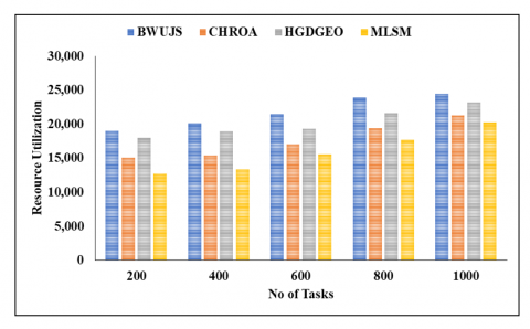
In this section, the presentation of MLSM is tested with existing techniques such as BWUJS [21], CHROA [29] and HGDGEO [30], where all models are implemented and results are averaged. The metrics such as resource utilization, total energy consumption, makespan, degree of imbalance and priority are used for proposed models’ effectiveness. Figures 2-6 presents the visual representation of various models in terms of different metrics.
Figure 2. Graphical description of projected model in terms of resource utilization
In Figure 2, the graphical representation of the projected model in terms of resource utilization is illustrated. In the analysis involving 200 tasks, the BWUJS model achieved a resource utilization of 18,972, while the CHROA model reached 15,101, the HGDGEO model reached 17,995, and the MLSM model reached 12,739, respectively.
For 600 tasks, the BWUJS model reached a resource utilization of 21,419, the CHROA model reached 17,047, the HGDGEO model reached 19,323, and the MLSM model reached 15,538, respectively.
For 800 tasks, the BWUJS model reached a resource utilization of 23,874, the CHROA model reached 19,410, the HGDGEO model reached 21,567, and the MLSM model reached 17,688, respectively.
Finally, for 1000 tasks, the BWUJS model achieved a resource utilization of 24,404, the CHROA model reached 21,265, the HGDGEO model reached 23,193, and the MLSM model reached 20,225, respectively.
Figure 3 signifies the visual representation of various models. In the analysis of 200 tasks, the BWUJS model reached a total energy consumption of 10.70, the CHROA model reached 10.05, the HGDGEO model reached 8.55, and the MLSM model reached a consumption of 6.84, respectively.
Figure 3. Visual representation of various models
For 400 tasks, the BWUJS model reached a total energy consumption of 13.82, the CHROA model reached 10.71, the HGDGEO model reached 8.94, and the MLSM model reached a consumption of 8.03, respectively.
For 600 tasks, the BWUJS model reached a total energy consumption of 17.65, the CHROA model reached 15.28, the HGDGEO model reached 12.02, and the MLSM model reached a consumption of 10.07, respectively.
For 800 tasks, the BWUJS model reached a total energy consumption of 19.94, the CHROA model reached 18.91, the HGDGEO model reached 15.26, and the MLSM model reached a consumption of 11.12, respectively.
Finally, for 1000 tasks, the BWUJS model reached a total energy consumption of 21.28, the CHROA model reached 19.56, the HGDGEO model reached 15.82, and the MLSM model reached a consumption of 13.84, respectively.
Figure 4 signifies the graphical representation of various models. In the analysis of 200 tasks, the BWUJS model reached a priority value of 39.04, the CHROA model reached 40.28, the HGDGEO model reached 52.75, and the MLSM model reached a consumption of 61.36, respectively.
For 400 tasks, the BWUJS model reached a priority of 46.45, the CHROA model reached 47.65, the HGDGEO model reached 57.35, and the MLSM model reached a consumption of 66.96, respectively.
For 600 tasks, the BWUJS model reached a priority of 51.24, the CHROA model reached 51.72, the HGDGEO model reached 61.23, and the MLSM model reached a consumption of 69.59, respectively.
For 800 tasks, the BWUJS model reached a priority of 54.21, the CHROA model reached 56.19, the HGDGEO model reached 65.75, and the MLSM model reached a consumption of 75.27, respectively.
Finally, for 1000 tasks, the BWUJS model reached a priority of 60.36, the CHROA model reached 60.48, the HGDGEO model reached 67.85, and the MLSM model reached a consumption of 77.43, respectively.
Figure 4. Graphical description of various models
The visual description of various models in terms of imbalance is indicated in Figure 5. When analyzing 200 tasks, the BWUJS model achieved a degree of imbalance of 8.742, the CHROA model reached 6.075, the HGDGEO model reached 5.720, and the MLSM model reached 3.570, respectively.
For 400 tasks, the BWUJS, CHROA, HGDGEO, and MLSM models reached degrees of imbalance of 10.874, 8.734, 5.830, and 4.160, respectively.
Subsequently, for 600 tasks, the MLSM model achieved a degree of imbalance of 4.740, while the BWUJS and CHROA models reached degrees of imbalance of 10.720 and 6.600, respectively.
For 800 tasks, the BWUJS model achieved a degree of imbalance of 15.595, the CHROA model reached 13.460, the HGDGEO model reached 8.830, and the MLSM model reached 5.390, respectively.
Finally, for 1000 tasks, the BWUJS model reached a degree of imbalance of 15.813, the CHROA model reached 14.830, the HGDGEO model reached 8.350, and the MLSM model reached 6.110, respectively.
Figure 5. Visual description of different models in terms of degree of imbalance
The efficiency of the suggested model is described in terms of makespan in Figure 6. The BWUJS model achieved a makespan of 2.938 in the analysis of 200 tasks, followed by the CHROA model at 1.764, 1.431, and the MLSM model at 1.136, in that order.
Figure 6. Description of anticipated model’s efficiency in terms of makespan
Next, for 400 tasks, the models from BWUJS and CHROA reached makespans of 2.935 and 2.567, 2.134, respectively, and lastly, the MLSM model reached a makespan of 1.742.
After that, for 600 tasks, the BWUJS model achieved a makespan of 7.937, the CHROA model reached makespans of 5.482 and 4.390, and the MLSM model, in turn, reached a makespan of 3.589.
Subsequently, for 800 tasks, the BWUJS model achieved a makespan of 9.942, the CHROA model reached makespans of 8.610 and 6.492, and the MLSM model achieved a makespan of 4.571.
Following that, for 1000 tasks, the BWUJS model achieved a makespan of 13.945, the CHROA model reached makespans of 11.490 and 8.481, and the MLSM model, in turn, reached a makespan of 5.896.
Finally, from the result evaluation, it is shown that the proposed model achieved better performance than existing techniques in terms of different metrics. The next section will describe the contribution of the research work.
Currently, Internet of Things (IoT) technology has great promise as a game-changing innovation. One of the several issues that must be resolved in the current paradigm of human-thing communication is the feasibility of software testing in environments that are as near to real as possible. Docker and container virtualization are well-suited to software development and testing in the IoT domain, according to the findings of the done study. Process isolation in containers improves the security of IoT devices, opens up new possibilities for virtual environment setups, enables more extensive and comprehensive testing of developed software, and decreases the number of faults.
A tiny containerisation clusters platform could be utilised for a range of IoT edge data processing submissions. Container orchestration and Docker's lightweight containerisation capabilities enable a regulated and fault-tolerant architecture for the edge. By continuously monitoring the state of the services, Docker's swarm ensures great service availability, which in turn enables the cluster to self-heal and scale. Even when dealing with massive quantities of data, the overall cost of the infrastructure may be kept down by using devices, which have a negligible impact on energy besides cost while still running complex infrastructures through clustering. The constraints of our prototype system are a result of the Big Data systems may be built on clusters of devices with very limited networking besides processing resources, such Raspberry Pis. The speed concerns experienced by the prototype approach were a result of using HDFS as a streaming data source.
An analysis of the container placement approach in cluster is presented in this research. Our goal is to assign containers to worker nodes that have the most efficient use of their resources. In this work, we provide MLSM, an approach that takes into account the present state of each node's resources as well as the different resource needs from containers. Additionally, this research suggests a better technique that combines cuckoo filters to increase space complexity, and it employs cuckoo filters as a linked list. We ran comprehensive tests using MLSM on the Docker Swarmkit platform. Comparisons with the default Spread method reveal substantial improvements in system stability and scalability. In light of the findings of this study and further research, cuckoo filters can be implemented into popular databases to enhance their query performance in analytics-centric domains. On average, including trade-offs into analytical systems won't reduce efficiency, but it will enhance space complexity, reduce the likelihood of false positives after deletions, and ensure consistent merges between cuckoo filters with low load factors.
[1] Volk, M., Staegemann, D., Islam, A., Turowski, K. (2022). Facing big data system architecture deployments: Towards an automated approach using container technologies for rapid prototyping. AIS eLibrary.
[2] Ahmad, I., AlFailakawi, M.G., AlMutawa, A., Alsalman, L. (2022). Container scheduling techniques: A survey and assessment. Journal of King Saud University-Computer and Information Sciences, 34(7): 3934-3947. https://doi.org/10.1016/j.jksuci.2021.03.002
[3] Mailewa, A., Mengel, S., Gittner, L., Khan, H. (2022). Mechanisms and techniques to enhance the security of big data analytic framework with mongodb and Linux containers. Array, 15: 100236. https://doi.org/10.1016/j.array.2022.100236
[4] Acharya, J., Suthar, A.C. (2022). Container scheduling algorithm in docker based cloud. Webology, 19(2).
[5] Hoang, V., Hung, L.H., Perez, D., Deng, H., Schooley, R., Arumilli, N., Yeung, K.Y., Lloyd, W. (2023). Container Profiler: Profiling resource utilization of containerized big data pipelines. GigaScience, 12: giad069. https://doi.org/10.1093/gigascience/giad069
[6] Pandey, B., Mishra, A.K., Yadav, A., Tiwari, D., Pandey, M.S. (2022). Virtualization using docker container. In Emerging Real-World Applications of Internet of Things. CRC Press, pp. 157-181.
[7] Vennu, V.K., Yepuru, S.R. (2022). A performance study for autoscaling big data analytics containerized applications: Scalability of apache spark on kubernetes. Digitala Vetenskapliga Arkivet.
[8] Bentaleb, O., Belloum, A.S., Sebaa, A., El-Maouhab, A. (2022). Containerization technologies: Taxonomies, applications and challenges. The Journal of Supercomputing, 78(1): 1144-1181. https://doi.org/10.1007/s11227-021-03914-1
[9] Kaiser, S., Haq, M.S., Tosun, A.Ş., Korkmaz, T. (2022). Container technologies for arm architecture: A comprehensive survey of the state-of-the-art. IEEE Access, 10: 84853-84881. https://doi.org/10.1109/ACCESS.2022.3197151
[10] EG, R., Bhaarath, J., Naveen, Nirmal, R. (2022). Docker container based crowd control analysis using dask hadoop framework. In Proceedings of the 6th International Conference on Information System and Data Mining, pp. 7-12. https://doi.org/10.1145/3546157.3546159
[11] Hernández-Rivas, A., Morales-Rocha, V., Ruiz-Hernández, O. (2023). Big data platform as a service for anomaly detection. In Data Analytics and Computational Intelligence: Novel Models, Algorithms and Applications. Cham: Springer Nature Switzerland, pp. 141-155. https://doi.org/10.1007/978-3-031-38325-0_7
[12] Petrosyan, D., Astsatryan, H. (2022). Serverless high-performance computing over cloud. Cybernetics and Information Technologies, 22(3): 82-92. https://doi.org/10.2478/cait-2022-0029
[13] Malviya, A., Dwivedi, R.K. (2022). A comparative analysis of container orchestration tools in cloud computing. In 2022 9th International Conference on Computing for Sustainable Global Development (INDIACom), New Delhi, India, pp. 698-703. https://doi.org/10.23919/INDIACom54597.2022.9763171
[14] Chiang, R.C. (2023). Contention-aware container placement strategy for docker swarm with machine learning based clustering algorithms. Cluster Computing, 26(1): 13-23. https://doi.org/10.1007/s10586-020-03210-2
[15] Thirumalraj, A., Chandrashekar, R., kavin Balasubramanian, P. (2024). Detection of pepper plant leaf disease detection using tom and jerry algorithm with MSTNet. In Machine Learning Techniques and Industry Applications. IGI Global Scientific Publishing, pp. 143-168. https://doi.org/10.4018/979-8-3693-5271-7.ch008
[16] Kim, B.S., Lee, S.H., Lee, Y.R., Park, Y.H., Jeong, J. (2022). Design and implementation of cloud docker application architecture based on machine learning in container management for smart manufacturing. Applied Sciences, 12(13): 6737. https://doi.org/10.3390/app12136737
[17] Naik, N. (2022). Cloud-agnostic and lightweight big data processing platform in multiple clouds using docker swarm and terraform. In Advances in Computational Intelligence Systems: Contributions Presented at the 20th UK Workshop on Computational Intelligence, September 8-10, 2021, Aberystwyth, Wales, UK 20. Springer International Publishing, pp. 519-531. https://doi.org/10.1007/978-3-030-87094-2_46
[18] Penchalaiah, N., Al-Humaimeedy, A.S., Maashi, M., Babu, J.C., Khalaf, O.I., Aldhyani, T.H. (2022). Clustered single-Board devices with docker container big stream processing architecture. Computers, Materials & Continua, 73(3): 5349. https://doi.org/10.32604/cmc.2022.029639
[19] Thirumalraj, A., Anandhi, R.J., Revathi, V., Stephe, S. (2024). Supply chain management using fermatean fuzzy-based decision making with ISSOA. In Convergence of Industry 4.0 and Supply Chain Sustainability. IGI Global, pp. 296-318. https://doi.org/10.4018/979-8-3693-1363-3.ch011
[20] Singh, N., Hamid, Y., Juneja, S., Srivastava, G., Dhiman, G., Gadekallu, T.R., Shah, M.A. (2023). Load balancing and service discovery using docker swarm for microservice based big data applications. Journal of Cloud Computing, 12(1): 4. https://doi.org/10.1186/s13677-022-00358-7
[21] Vasantham, V.K., Donavalli, H. (2024). Multi-objective hybrid optimized task scheduling in cloud computing under big data perspective. Intelligent Decision Technologies, 18(2): 1287-1303. https://doi.org/10.3233/IDT-230717
[22] Yang, W. (2024). Analysis and application of big data feature extraction based on improved k-means algorithm. Scalable Computing: Practice and Experience, 25(1): 137-145. https://doi.org/10.12694/scpe.v25i1.2281
[23] Sun, D., Zhang, C., Gao, S., Buyya, R. (2024). An adaptive load balancing strategy for stateful join operator in skewed data stream environments. Future Generation Computer Systems, 152: 138-151. https://doi.org/10.1016/j.future.2023.11.002
[24] Ananthi, M., Gopal, A., Ramalakshmi, K., Mohan Kumar, P. (2024). Gaussian adapted markov model with overhauled fluctuation analysis-based big data streaming model in cloud. Big Data, 12(1): 1-18. https://doi.org/10.1089/big.2023.0035
[25] Singh, K.D., Singh, P.D. (2024). QoS‐enhanced load balancing strategies for metaverse‐infused VR/AR in engineering education 5.0. Computer Applications in Engineering Education, 32(3): e22722. https://doi.org/10.1002/cae.22722
[26] Sharma, A., Balasubramanian, V., Kamruzzaman, J. (2024). A temporal deep Q learning for optimal load balancing in software-defined networks. Sensors, 24(4): 1216. https://doi.org/10.3390/s24041216
[27] Khan, M.I., Sharma, K. (2024). An efficient nature-inspired optimization method for cloud load balancing for enhanced resource utilization. International Journal of Intelligent Systems and Applications in Engineering, 12(7s): 560-571.
[28] Liu, S., He, M., Wu, Z., Lu, P., Gu, W. (2024). Spatial-temporal graph neural network traffic prediction-based load balancing with reinforcement learning in cellular networks. Information Fusion, 103: 102079. https://doi.org/10.1016/j.inffus.2023.102079
[29] Aqeel, I., Khormi, I.M., Khan, S.B., Shuaib, M., Almusharraf, A., Alam, S., Alkhaldi, N.A. (2023). Load balancing using artificial intelligence for cloud-enabled internet of everything in healthcare domain. Sensors, 23(11): 5349. https://doi.org/10.3390/s23115349
[30] Jagadish Kumar, N., Balasubramanian, C. (2023). Hybrid gradient descent golden eagle optimization (HGDGEO) algorithm-based efficient heterogeneous resource scheduling for big data processing on clouds. Wireless Personal Communications, 129(2): 1175-1195. https://doi.org/10.1007/s11277-023-10182-0
[31] Chen, M., Mao, S., Zhang, Y., Leung, V.C.M. (2014). Big data analysis. In Big Data. Springer, pp. 51-58. https://doi.org/10.1007/978-3-319-06245-7_5
[32] Naik, N. (2017). Docker container-based big data processing system in multiple clouds for everyone. In 2017 IEEE International Systems Engineering Symposium (ISSE), Vienna, Austria, pp. 1-7. https://doi.org/10.1109/SysEng.2017.8088294
[33] Su, H., Zhao, D., Heidari, A.A., Liu, L., Zhang, X., Mafarja, M., Chen, H. (2023). RIME: A physics-based optimization. Neurocomputing, 532: 183-214. https://doi.org/10.1016/j.neucom.2023.02.010