María J. Aza-Espinosa![]() | Erick P. Herrera-Granda*
| Erick P. Herrera-Granda*![]() | Marcelo Ibarra-Rosero
| Marcelo Ibarra-Rosero![]()
© 2023 IIETA. This article is published by IIETA and is licensed under the CC BY 4.0 license (http://creativecommons.org/licenses/by/4.0/).
OPEN ACCESS
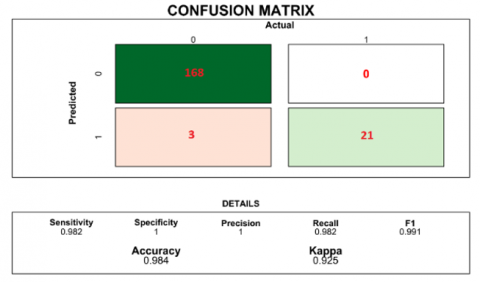
An automated risk model for Brucellosis detection in cattle farms, termed DeepBrucel, was developed and validated. A comprehensive survey encompassing 51 variables related to farm characteristics, management practices, and reproductive pathologies was administered across 632 cattle farms in Ecuador. The extensive dataset thus obtained was utilized to implement and compare classifiers based on regression, neural networks, and deep learning methodologies. A wide-ranging primary experimentation protocol enabled the identification of critical variables and the optimal topology for the neural networks. Superior performance was exhibited by a deep neural network model with three hidden layers, which achieved an impressive accuracy of 98.4% in predicting Brucellosis risk. DeepBrucel, now publicly available, provides a highly accessible and robust tool for the diagnosis and control of Brucellosis in cattle farms.
automatic brucellosis diagnosis, Neural Networks Brucellosis Diagnosis, multivariate diagnostic techniques
Brucellosis, a contagious disease primarily affecting livestock, has emerged as a global health concern. This infectious disease inflicts a significant toll on livestock, including cattle, goats, sheep, and pigs, resulting in adverse effects such as abortion, infertility, decreased milk production, and mortality [1]. It is primarily transmitted through ingestion of contaminated pasture, food, water, or through contact with infected animal excretions or vaginal secretions. The significant prevalence of Brucellosis, especially in regions like the province of Carchi, where it ranges from 1.97% to 10.62%, underscores the magnitude of the problem [2]. The challenges in distinguishing vaccinated animals from infected ones using serological tests, coupled with the high cost and limited control of vaccines, have exacerbated the problem.
The current endeavor intends to address these issues by introducing an automated diagnostic mechanism to assess the risk of Brucellosis in cattle farms in the Carchi province. This study builds upon previous research [3] that identified relevant risk factors, employing a multivariate approach to develop an automatic model that determines Brucellosis risk.
1.1 Related work
There is a substantial body of literature on Brucellosis, focusing on identifying risk factors, seroprevalence, and management practices associated with the disease. An early study [4] employed univariate and multivariate statistical methods to identify clinical predictors for relapse in patients with Brucellosis. The study discovered a 67% relapse rate within 12 months, emphasizing the need for additional care in high-risk patients.
Peng et al. [5] used ArcGIS software to analyze the incidence rate of Brucellosis in China over time. It revealed that sheep inventory, GDP, and climate were significantly correlated with Brucellosis incidence. Furthermore, a study conducted in Pakistan used Pearson's Chi-square test and deep learning techniques to correlate epidemiological data with test results [6]. This study achieved over 83% accuracy in classifying and prioritizing the main risk factors associated with Brucellosis. In Algeria, a multivariate analysis found a 3.49% seroprevalence in the bovines tested, with common feeders in pastures and intensive livestock being the main risk factors for tuberculosis transmission [7]. In addition, a comprehensive investigation was executed across five districts, encompassing a total sample pool of 1907 subjects selected from 212 herds [8]. Blood specimens were procured from the cattle, with seropositivity scrutinized using the Rose Bengal test, and validation was performed through indirect ELISA. A comprehensive evaluation of risk factors was facilitated by administering questionnaires, coupled with the application of Chi-square and Fisher's Exact Test, as well as multivariate logistic regression analysis. The study unveiled a seroprevalence of 13.6% and identified a host of risk factors. These encompassed the education level of the owners, the incorporation of new animals into the herd, interaction with small ruminants, a history of abortions, advanced age of the animals, and a pronounced lack of disease awareness amongst cattle owners.
Sil et al. [9] focused on the use of advanced techniques for disease detection, as demonstrated by a study that employed a microspectroscopic vibrational Raman technique combined with multivariate analysis and deep learning to detect Brucella and Bacillus pathogens based on DNA analysis. The researchers achieved 96.33% accuracy using a convolutional neural network (CNN) architecture.
Furthermore, studies have been conducted to evaluate risk factors in specific regions, such as a study in Hisar, India, which identified the presence of other animals in the herd, particularly sheep and goats, and the use of a common water source as significant Brucellosis risk factors [10]. A similar study in the Ludhiana district in Punjab found that 17.9% of cows and 11.9% of buffaloes tested positive for Brucella [11].
Moreover, an estimated seroprevalence of 9.7% was reported among individuals with direct contact with cattle [12]. In a study conducted in Fayoun, Upper Egypt, the incidence of Brucellosis in both humans and cattle was investigated. Logistic regression analysis illuminated an elevated probability of Brucellosis in illiterate individuals, those employed in livestock-related occupations, those with an infected family member, and those with a familial history of the disease. The study further revealed that domestic cattle rearing and exposure to bovine abortions without adequate protective measures were significant risk factors. The consumption of raw milk and homemade cheese demonstrated significance in the univariate model, with the latter being strongly associated with Brucellosis in the multivariate model. Molecular genotyping disclosed the presence of various genotypes, with G6 being the reference strain for Brucella melitensis.
Subsequently, a study encompassing 740 dairy animals from 534 households across 52 villages in Bihar and Assam was instigated [13]. The application of serological tests using iELISA yielded a positivity rate of 15.9% in Assam and 0.3% in Bihar. Analysis of risk factors was facilitated through a survey and statistical tests, including Chi-square, T-tests, and logistic regression. The study identified significant risk factors such as the location of artificial insemination, age, and management practices.
Research into Brucellosis persists to be a focal point of exploration. In 2022, a seroprevalence study and evaluation of risk factors were conducted in the Jimma region of Ethiopia, with data from 424 bovine blood samples and 114 households being scrutinized [14]. Univariate analysis with a Chi-square test and multivariate logistic regression models were employed to investigate the relationship between seropositivity and risk factors. The study identified seropositive animals predominantly as adults of the local breed, and it unveiled a significant association between body condition, pregnancy, abortion, and reproduction. The analysis also reported higher seroprevalence in animals managed under extensive systems and in contact with other pregnant bovines.
Simultaneously, Male Here et al. [15] delineated a study conducted in Ireland, utilizing data from 6,611,854 slaughtered animals. Logistic regression models were applied to analyze the risk of tuberculosis confirmation lesions in factory injuries. Purchased animals presented a higher risk of confirmation than those raised domestically. Small herds, lactating dairy herds, and herds with a history of tuberculosis were associated with an increased probability of confirming tuberculosis lesions.
Conversely, a study executed in Egyptian governorates examined 400 bovine samples using serological analysis with an iELISA kit [16]. Risk factors were identified through farm and owner registration, and the data were analyzed using logistic regression and classification and regression trees (CART).
The study uncovered a 65.5% seroprevalence in bovines raised in herds exceeding 100 animals and significant associations with factors such as disinfection following birth, abortion history, and shared equipment use.
The research approach was directed in a mixed way (quantitative and qualitative), favoring broad methodologies that reinforce multimodal designs and allow a broader vision of the subject studied. In the first qualitative point, the appropriate variables that will be entered into the different multivariate techniques models as training data were selected based on previous studies will additionally induce a quantitative approach allowing statistical analysis to determine risk percentage so that farms implement actions to control this pathology. In addition, the qualitative approach is part of this research in an in-depth analysis of the results obtained from implementing different models, determining advantages, limitations selecting the best alternative for the pathology automatic diagnosis.
2.1 Study site and sample collection
The present investigation was carried out in the Tulcán-Carchi Province, where ten parishes of the canton were evaluated, of which 600 samples were analyzed, conducting a survey applied to the owners of the different locations of livestock exploitation taking into account the progressive increase of Brucellosis being a risk factor for animals and humans due to their interaction causing a great impact at an economic, social and health levels.
2.2 Survey instrument and variables
The instrument was built using associated risk factors identified in previous studies [2, 3], where it was possible to determine, as a first point of interest (factor), location exploitation taking into account the parish and the number of people working-data will allow locating geographical area and activities carried out on the farm. As a second point of interest, the general data of the farm was addressed, taking into account surface, farm type, production, other animals, breed, and number of cattle heads for inventory purposes and to know if the animals were treated separately in addition to find out breeds or quantity that pose greater Brucellosis infection susceptibility. The third point is farm generalities, considering restrictions on the property entry, determining hygiene mechanisms and restrictions on individuals who may be carrying the bacteria. In addition, food origin and water source was recorded as untreated water maybe a disease transmission mechanism. The fourth point addressed was the production system considering bull semen origin, calving place and disinfection since hygiene is of vital importance to prevent direct contagion with workers and cows whether the place is free of possible infections. As a fifth point, reproductive pathology was considered, taking abortions into account. Metritis was recorded in sick animals since this is a known risk factor for Brucella. As a sixth and seventh point, the diagnosis and sanitary calendar were recorded, whether there are tests, samples, and preventive control measures. In addition, the vaccination schedule was considered since commonly having a record of each bovine's condition makes disease detecting treatment easier. The eighth and ninth point is the milking and workers data since quality expertise parameters and equipment disinfection are taken into account as workers may be in direct contact with the bovine posing direct contamination risks. As the tenth point is the risk of food consumption Whether workers are aware of the disease although Brucellosis depends to a large extent on animals, the human being is an accidental host at product consumption becoming a carrier of this pathology.
As mentioned before, the instrument was created based on previous studies results [2, 3], where relevant key risk factors were selected based on a literature review. Then they were structured in a survey and validated using classic statistical techniques: Confirmatory Factorial Analysis, Regressions for the ordinal, categorical, and numeric variables, respectively [2, 3]. This way, 51 variables were classified as representative regressors for the Brucellosis risk variable. Variables that comprised the instrument are presented in Table 1.
Table 1. Instrument variables
|
Factor |
Code |
Variable |
|
Location |
q1 |
Canton |
|
Farm description |
q2 |
Total area |
|
q3 |
Exploitation type |
|
|
q4 |
Number of cattle |
|
|
q5 |
Cattle breed |
|
|
q6 |
Inventory of other animals |
|
|
Farm generalities |
q7 |
Restriction on the entry of individuals. |
|
q8 |
Source of replacement animals |
|
|
q9 |
Where does the drinking water for the animals come from? |
|
|
q10 |
Feeding system |
|
|
q11 |
Use of organic waste to fertilize the pastures |
|
|
Production system |
q12 |
Reproductive system employed |
|
q13 |
Origin of the bull |
|
|
q14 |
Where does the semen used come from? |
|
|
q15 |
Percentages of cows in your herd that are primiparous |
|
|
q16 |
There is a specific place for births |
|
|
q17 |
Do you disinfect the farrowing pens? |
|
|
Reproductive pathology |
q18 |
Do the cows in your herd miscarry? |
|
q19 |
What is the fate of the aborted tissues? |
|
|
q20 |
What is the fate of sick animals? |
|
|
q21 |
Is there metritis in animals? |
|
|
Diagnosis |
q22 |
Are diagnostic tests performed? |
|
q23 |
Has Brucellosis been diagnosed in your herd? |
|
|
q24 |
In which species was the sample taken? |
|
|
q25 |
What preventive and control measures were taken? |
|
|
Sanitary calendar |
q26 |
Is there a vaccination schedule? |
|
q27 |
Do you vaccinate animals against Brucellosis? |
|
|
q28 |
What type of vaccine was used? |
|
|
q29 |
what kind of animals are vaccinated? |
|
|
Milking |
q30 |
What type of milking do you use? |
|
q31 |
Do you know the quality parameters of your herd's milk? |
|
|
q32 |
Is disinfection of equipment hands and udders carried out? |
|
|
Workers data |
q33 |
What type of activity is carried out in your herd? |
|
q34 |
Is there a periodic medical check-up of the workers? |
|
|
q35 |
Have you been tested for Brucellosis? |
|
|
q36 |
Have there been abortions in your family? |
|
|
q37 |
What animals have you had contact with? |
|
|
q38 |
Have you had contact with placentas, fetuses, or secretions? |
|
|
q39 |
Do you use any type of protection at work? |
|
|
Food consumption risk |
q40 |
What kind of cow's milk do you drink? |
|
q41 |
What kind of yogurt do you eat? |
|
|
q42 |
What kind of cheese do you eat? |
|
|
q43 |
What kind of butter do you eat? |
|
|
q44 |
Is self-consumption of milk carried out in the APU? |
|
|
q45 |
Do you make products from the milk produced? |
|
|
q46 |
Do you know what Brucellosis is? |
|
|
q47 |
Do you know how Brucellosis is transmitted? |
|
|
q48 |
Do you know what the symptoms are in humans? |
|
|
q49 |
Do you know what the symptoms are in animals? |
|
|
q50 |
Has any family member had Brucellosis? |
|
|
q51 |
Do you know of any control program for this disease? |
2.3 Data analysis
Database compilation for any study is susceptible to including missing data and outliers, which is why it is recommended that all statistical analysis begins with applying a data analysis protocol. Among the most used techniques for data treatment for multivariate samples are Mahalanobis distances. This technique allows the measurement of the number of standard deviations in which an observation is located concerning the mean in a distribution; since outliers do not behave similarly to common observations, this measure can be used to detect outliers. From a geometric point of view, the Euclidean distance is the shortest distance between two points; however, the correlation between highly correlated variables isn’t considered. The difference between the Mahalanobis distance and the Euclidean distance is that it does value the correlation between variables [17, 18]. This is a scale-invariant metric contemplating the distance between a point generated by an $\boldsymbol{x} \in \mathbb{R}^p$, p-varied probability distribution fX(.) and the mean μ=E(X) in the distribution. Assuming that the distribution fX(.) has finite moments of second order, the covariance matrix can be determined as ∑=E(X-μ). Thus, the Mahalanobis distances are defined as:
$D(\boldsymbol{X}, \mu)=\sqrt{(\boldsymbol{X}-\mu)^T \Sigma^{-1}(\boldsymbol{X}-\mu)}$ (1)
2.4 Modeling techniques
2.4.1 Principal component analysis
The principal component analysis is a dimension reduction technique where a group of correlated variables is intended to become a shorter group of uncorrelated variables. Principal Component Analysis (PCA) is commonly used as an exploratory data analysis technique, examining the relationship between a group of variables, so it can be used as a dimension reduction technique [19]. Furthermore, as described in the studies [20, 21], the PCA can be used to determine the number of hidden layers that must be implemented in a neural network. For a dataset x(1), x(2),⋯, x(m) with n-dimensional observations, it is intended to reduce the dataset to k-dimensional observations (when k<n). Therefore, the process begins with data standardization:
$x_j^i=\frac{x_j^i-\bar{x}_j}{\sigma_j}$ (2)
Then, the covariance matrix is calculated using the following:
$\Sigma=\frac{1}{m} \sum_i^m\left(x_i\right)\left(x_i\right)^T, \Sigma \in \mathbb{R}^{n \times n}$ (3)
Next, covariance matrix eigenvector and eigenvalue are obtained using the equation:
$\begin{aligned} & u^T \Sigma=\lambda \mu, \\ & U=\left[\begin{array}{ccc}\mid & \mid & \mid \\ u_1 & u_2 \ldots & u_n \\ \mid & \mid & \mid\end{array}\right], u_i \in \mathbb{R}^n \\ & \end{aligned}$ (4)
In this way, the original data is projected to a subspace of k-dimensions so that covariance matrix main eigenvectors are selected. These new variables represent original data and its variance. Each of these new vectors can be obtained using the expression:
$x_i^{\text {new }}=\left[\begin{array}{c}u_1^T x^i \\ u_2^T x^i \\ \vdots \\ u_k^T x^i\end{array}\right] \in \mathbb{R}^k$ (5)
In particular, PCA is a useful tool for neural networks model design because, as mentioned in the studies [20, 21], it can be applied to determine how many necessary components explain a significant amount of the variance observed in the dataset, equivalent to the number of hidden layers of the network. A good rule of thumb is to consider at least a higher number of hidden layers as components are required to explain 70% of dataset total variance [21].
2.4.2 Neural networks
Neural networks, as a classification technique, constitute an assembly method in which each artificial neuron emulates the behavior of a biological neuron by combining a set of weights at input, activating and transmitting a signal only if the input signal combination is large enough to reach a threshold. There is a large number of activation functions that can be selected for the functioning of each neuron. However, in the present work, we selected the RELU (Rectified Linear Unit) $\operatorname{Re} L U \rightarrow \sigma=\max (0, z)$ to design the hidden layers and the SoftMax SoftMax $\rightarrow \sigma=e^{z_j} / \sum_i e^{z_i}$ for the output layer that must have a binary behavior. Artificial neural networks constitute an assembly technique that can enter as many input variables as necessary, employing a neuron in the input layer commonly not provided with an activation function. Subsequently, as many links as necessary are generated, where a weight wi,j is assigned for each link, which is a parameter that will be estimated through the learning process, activating or not neurons different combinations of the hidden and output layers, thus allowing each neuron or combinations to learn non-linear behaviors from data. The expression obtains the signal propagation process in each layer of the neural network:
$\boldsymbol{X}_j=\boldsymbol{W}_{i j} \cdot \boldsymbol{I}$ (6)
$\boldsymbol{\mathcal { O }}_j=\operatorname{activation}\left(\boldsymbol{X}_j\right)$ (7)
where, Xj represents the matrix of total input signals from the neurons of a j layer neural network, Wij represents the matrix of weights of existing links between the current layer j and the previous layer i, I is the matrix of input signals and $\boldsymbol{\mathcal { O }}_j$ represents the matrix of output signals from each neural network layer. Determining the learning of a neural network, error $e_{\text {out }_k}=t_k-\sigma_k$ of each neuron of the final layer is calculated by comparing the obtained value y with the expected value for each observation t. These errors must be back-propagated through the neural network links where each output comes from to allow weights update. Errors can be back-propagated in the neural network using the expression:
$\xi_i=\boldsymbol{W}_{i j}^T \cdot \xi_j$ (8)
where, ξi represents the matrix of errors that will be back-propagated to the previous layer of the neural network and ξj are errors coming from the next neural network layer. Once the errors are backpropagated in the neural network, these weights allow the neural network to retain information from previous examples adding new information from new observations. One of the most widely used processes for this purpose is gradient descent formulated as follows:
$\frac{\partial \xi}{\partial \boldsymbol{W}_{j k}}=\frac{\partial \sum_n\left(t_n-\sigma_n\right)}{\partial \boldsymbol{W}_{j k}}=\frac{\partial \xi}{\partial \boldsymbol{\mathcal { O }}_k} \cdot \frac{\partial \boldsymbol{\mathcal { O }}_k}{\partial \boldsymbol{W}_{j k}}=-2\left(t_n-\sigma_n\right) \cdot \frac{\partial \boldsymbol{\mathcal { O }}_k}{\partial \boldsymbol{W}_{j k}}$ (9)
where, $\boldsymbol{W}_{j k}^{(r+1)}$ represents the new updated weight for a link jk, updated from its previous value $\boldsymbol{W}_{j k}^{(r)}$, and the gradient ∂ξ/∂Wjk that enters a new portion of information moderated by the Learning-rate hyper-parameter α [22-24].
2.4.3 Deep learning
Artificial neural networks having two or more hidden layers with consecutive non-linear activation functions are called Deep Learning models [22]. However, excessive addition of hidden layers and a greater number of neurons is not always the best alternative leading the model to overfitting problems. In addition, calculating parameters involved in the model can become a challenging task since calculating the parameter update will involve a larger number of derivatives. This problem can be addressed by using the chain rule, which is stated as follows:
$\frac{d f_3}{d u}(x)=\frac{d f_3}{d u}\left(f_2\left(f_1(x)\right)\right) \times \frac{d f_2}{d u}\left(f_1(x)\right) \times \frac{d f_1}{d u}(x)$ (10)
Example, for a Deep Learning model with two hidden layers, in addition to the matrix of weights Wk involved in each layer, a Bias term can be added as an intercept Bk. The concept of a two-hidden-layer model is presented in Figure 1.
Figure 1. Two hidden layers deep learning model formulation
Following the proposed formulation, the gradients used for weight update in the neural network connections can be calculated using the expressions:
$\frac{\partial L}{\partial B_2}=\frac{\partial \lambda}{\partial P}(P, Y) \times \frac{\partial \psi}{\partial B_2}\left(M_2, B_2\right)$ (11)
$\frac{\partial L}{\partial W_2}=\frac{\partial \lambda}{\partial P}(P, Y) \times \frac{\partial \psi}{\partial M_2}\left(M_2, B_2\right) \times \frac{\partial \rho}{\partial W_2}\left(O_1, W_2\right)$ (12)
$\begin{aligned} \frac{\partial L}{\partial B_1}=\frac{\partial \lambda}{\partial P}(P, Y) \times & \frac{\partial \psi}{\partial M_2}\left(M_2, B_2\right) \times \frac{\partial \rho}{\partial M_1}\left(O_1, W_2\right) \\ & \times \frac{\partial \beta}{\partial M_1}\left(N_1\right) \times \frac{\partial \alpha}{\partial B_1}\left(M_1, B_1\right)\end{aligned}$ (13)
$\begin{aligned} \frac{\partial L}{\partial W_1}=\frac{\partial \lambda}{\partial P}(P, Y) & \times \frac{\partial \psi}{\partial M_2}\left(M_2, B_2\right) \times \frac{\partial \rho}{\partial M_1}\left(O_1, W_2\right) \\ & \times \frac{\partial \beta}{\partial M_1}\left(N_1\right) \times \frac{\partial \alpha}{\partial M_1}\left(M_1, B_1\right) \\ & \times \frac{\partial \gamma}{\partial W_1}\left(X, W_1\right)\end{aligned}$ (14)
Once the learning process and parameters update is configured, there is still an open question regarding the number of neurons retained in each hidden layer. There are many approaches tending to answer this open question, like formulas of: Li, Chow, and Yu, Tamura and Tateishi, Xu and Chen, Shibata and Ikeda method, Hunter, Yu, Pukish III, Kolbusz and Wilamowski, and the Sheela and Deepa, listed in the study of Vujičić et al. [25]. Nevertheless, given the large number of input neurons required in our method, we followed the recommendations of Demuth et al. [26], which consider all the possible configurations of neurons for the hidden layer, from half to twice the number input layer neurons. This procedure involves harder experimentation work but ensures an appropriate search interval to guarantee the finding of a good model.
2.4.4 Model validation
For model validation, the dataset was split into training and test datasets, used to verifying the performance of each classification model when trying to predict unseen data outcome. For this purpose, the rule of thumb rule was applied for 70% proportional to the training data, and 30% was kept for validation purposes.
Once the training stage of each model finished, we extracted the classifier performance metrics using the confusion matrix. The confusion matrix is widely used as a performance evaluation tool for validating classification models. It provides a tabular representation of the predicted and actual classification models output types. The confusion matrix aids in understanding how well a classification model performs in correctly classifying instances into their respective classes. It provides a detailed breakdown of model's predictions, enabling pattern identification, biases, and errors. This information helps fine-tune the model, adjust classification thresholds, optimizing model performance for specific objectives or requirements. The matrix consists of four components: true positives (TP), true negatives (TN), false positives (FP), and false negatives (FN).
From these measures, some performance metrics can be calculated:
Precision. Also known as “positive predictive value”, measures the ratio of accurately predicted positive instances to the total number of positive predictions made by the detector.
precision $=\frac{T P}{T P+F P}$ (15)
Accuracy. This metric evaluates the overall success rate indicating algorithm effectiveness, representing the proportion of correct predictions.
accuracy $=\frac{T P+T N}{T P+F N+T N+F P}$ (16)
In addition, we considered two important metrics related to the error obtained in each prediction made over the unseen data.
MSE. MSE (Mean Squared Error) is a common performance metric in machine learning measuring the average squared difference between the predicted and actual values. It quantitatively measures the model's accuracy, with lower MSE values indicating better predictive performance.
$M S E=\frac{1}{n} \sum_{t=1}^{t=n}\left(y^{\prime}-y\right)^2$ (17)
Loss. Loss refers to the objective function quantifying the discrepancy between predicted output and true target value during training. It represents the error or cost incurred by the model and guides the optimization process minimizing the error improving model performance. For example, the categorical cross entropy Loss employed in the ML proposed models is defined as:
$\operatorname{Loss}_{C E}=-\sum_{i=1}^{i=N} y_i \cdot \log \left(y_i^{\prime}\right)$ (18)
The database used for the study consisted of 632 observations from a multivariate instrument comprising 51 variables, 21 of which were binary and 30 categorical. These variables were proposed by experts in Brucellosis studies [3], representing the risk factors involved in the presence of Brucellosis on cattle farms. Since the proposed instrument is of a categorical and ordinal multivariate nature, it is a complex problem to be dealt with using conventional statistical techniques. This is why in this study, artificial neural networks and Deep learning were selected as the main techniques due to the great advances and excellent results in recent years, especially for handling data composed of non-linear variables [23]. Additionally, the results were contrasted with logistic regression, selected as a classical statistical technique due to its high popularity and in the obtaining of classification models excellent results based on non-linear regressors.
The database was processed using the statistical programming language R, in conjunction with Python over the Anaconda distribution, allowing TensorFlow and Keras packages handling from RStudio, through the library reticulate. Data analysis began by imputing 127 missing data distributed throughout the database, representing 0.394% of the sample, a proportion that is significantly lower than 5%; therefore, the criterion was met, and KNN technique (K- Nearest Neighbors) was used to impute data through the library VIM.
Next, the coded categorical variables were used to detect outliers, for which the Mahalanobis Distances were used, obtained with respect to the data centroid. For this process, a 191.5196 cutoff score was defined based on χ2 conserving 99.9% distribution excluding 0.01% of furthest distance (outliers). In this way, no atypical observations were detected, so the database kept its 632 observations.
Then, the categorical and binary variables were transformed into Dummy type variables, depending on the parameter levels of each variable, using the recipes and tidyverse libraries. Thus, the coded database using dummy variables was made up of 125 variables, from which 124 were considered regressors (features) or data for the input neuron layer, and the variable brucelosisdiagnos (diagnosis of Brucellosis) was considered as the single response variable (labels). Additionally, the libraries GGally and skimr were used as data visualization mechanisms to verify the information before training the models. The results are presented in Table 2.
As seen in Table 2, through data processing, a database was obtained with no atypical or missing data, and each of the 124 regressor variables had a variance different from zero.
Table 2. Descriptive statistics of the coded variables in dummy format
|
Variable Name |
N.Missing |
Complete.Rate |
Num.Mean |
Num.Sd |
Num p0 |
Num p25 |
Num p50 |
Num p75 |
Num p100 |
Hist. |
|
canton tulcan |
0 |
1 |
0.2693662 |
0.44402157 |
0 |
0 |
0 |
1 |
1 |
▇▁▁▁▃ |
|
canton huaca |
0 |
1 |
0.10739437 |
0.30988689 |
0 |
0 |
0 |
0 |
1 |
▇▁▁▁▁ |
|
canton montufar |
0 |
1 |
0.24823944 |
0.43237223 |
0 |
0 |
0 |
0 |
1 |
▇▁▁▁▃ |
|
canton espejo |
0 |
1 |
0.16901408 |
0.37509469 |
0 |
0 |
0 |
0 |
1 |
▇▁▁▁▂ |
|
canton mira |
0 |
1 |
0.04753521 |
0.21296823 |
0 |
0 |
0 |
0 |
1 |
▇▁▁▁▁ |
|
canton bolivar |
0 |
1 |
0.1584507 |
0.36548496 |
0 |
0 |
0 |
0 |
1 |
▇▁▁▁▂ |
|
totalsurface 1a10hect |
0 |
1 |
0.88380282 |
0.3207437 |
0 |
1 |
1 |
1 |
1 |
▁▁▁▁▇ |
|
totalsurface 10a20hect |
0 |
1 |
0.05985915 |
0.23743481 |
0 |
0 |
0 |
0 |
1 |
▇▁▁▁▁ |
|
totalsurface 20a50hect |
0 |
1 |
0.01760563 |
0.13162895 |
0 |
0 |
0 |
0 |
1 |
▇▁▁▁▁ |
|
totalsurface morethan50h |
0 |
1 |
0.00176056 |
0.04195907 |
0 |
0 |
0 |
0 |
1 |
▇▁▁▁▁ |
|
exploittype intensive |
0 |
1 |
0.41021127 |
0.49230548 |
0 |
0 |
0 |
1 |
1 |
▇▁▁▁▆ |
|
exploittype extensive |
0 |
1 |
0.26760563 |
0.44310103 |
0 |
0 |
0 |
1 |
1 |
▇▁▁▁▃ |
|
exploittype mixed |
0 |
1 |
0.17605634 |
0.38120381 |
0 |
0 |
0 |
0 |
1 |
▇▁▁▁▂ |
|
productiontype milk |
0 |
1 |
0.79049296 |
0.40731552 |
0 |
1 |
1 |
1 |
1 |
▂▁▁▁▇ |
|
productiontype meat |
0 |
1 |
0.00352113 |
0.05928673 |
0 |
0 |
0 |
0 |
1 |
▇▁▁▁▁ |
|
productiontype mixed |
0 |
1 |
0.00528169 |
0.07254695 |
0 |
0 |
0 |
0 |
1 |
▇▁▁▁▁ |
|
productiontype others |
0 |
1 |
0.01056338 |
0.10232414 |
0 |
0 |
0 |
0 |
1 |
▇▁▁▁▁ |
|
cattlenumber 1to10 |
0 |
1 |
0.77640845 |
0.41701863 |
0 |
1 |
1 |
1 |
1 |
▂▁▁▁▇ |
|
cattlenumber 10to20 |
0 |
1 |
0.17957746 |
0.38417345 |
0 |
0 |
0 |
0 |
1 |
▇▁▁▁▂ |
|
cattlenumber 20to30 |
0 |
1 |
0.0193662 |
0.13792984 |
0 |
0 |
0 |
0 |
1 |
▇▁▁▁▁ |
|
cattlenumber 30to40 |
0 |
1 |
0.01232394 |
0.11042433 |
0 |
0 |
0 |
0 |
1 |
▇▁▁▁▁ |
|
cattlenumber 40to50 |
0 |
1 |
0.00352113 |
0.05928673 |
0 |
0 |
0 |
0 |
1 |
▇▁▁▁▁ |
|
cattlebreed holstein |
0 |
1 |
0.97535211 |
0.15518624 |
0 |
1 |
1 |
1 |
1 |
▁▁▁▁▇ |
|
cattlebreed jersey |
0 |
1 |
0.00704225 |
0.08369584 |
0 |
0 |
0 |
0 |
1 |
▇▁▁▁▁ |
|
cattlebreed f1 |
0 |
1 |
0.00528169 |
0.07254695 |
0 |
0 |
0 |
0 |
1 |
▇▁▁▁▁ |
|
cattlebreed brownsuiz |
0 |
1 |
0.00528169 |
0.07254695 |
0 |
0 |
0 |
0 |
1 |
▇▁▁▁▁ |
|
cattlebreed pizan |
0 |
1 |
0.00352113 |
0.05928673 |
0 |
0 |
0 |
0 |
1 |
▇▁▁▁▁ |
|
inventory sheep |
0 |
1 |
0.00880282 |
0.0934918 |
0 |
0 |
0 |
0 |
1 |
▇▁▁▁▁ |
|
inventory goats |
0 |
1 |
0.01056338 |
0.10232414 |
0 |
0 |
0 |
0 |
1 |
▇▁▁▁▁ |
|
inventory pigs |
0 |
1 |
0.38028169 |
0.4858839 |
0 |
0 |
0 |
1 |
1 |
▇▁▁▁▅ |
|
inventory dogs |
0 |
1 |
0.8028169 |
0.39822245 |
0 |
1 |
1 |
1 |
1 |
▂▁▁▁▇ |
|
inventory cats |
0 |
1 |
0.16549296 |
0.37195243 |
0 |
0 |
0 |
0 |
1 |
▇▁▁▁▂ |
|
inventory horses |
0 |
1 |
0.01408451 |
0.11794331 |
0 |
0 |
0 |
0 |
1 |
▇▁▁▁▃ |
|
inventory camelids |
0 |
1 |
0.00704225 |
0.08369584 |
0 |
0 |
0 |
0 |
1 |
▇▁▁▁▁ |
|
inventory others |
0 |
1 |
0.06338028 |
0.24386045 |
0 |
0 |
0 |
0 |
1 |
▇▁▁▁▁ |
|
restriction |
0 |
1 |
0.69542254 |
0.46063391 |
0 |
0 |
1 |
1 |
1 |
▃▁▁▁▇ |
|
provenance neighbor |
0 |
1 |
0.16373239 |
0.37035873 |
0 |
0 |
0 |
0 |
1 |
▇▁▁▁▂ |
|
provenance locality |
0 |
1 |
0.32394366 |
0.46839131 |
0 |
0 |
0 |
1 |
1 |
▇▁▁▁▃ |
|
provenance fair |
0 |
1 |
0.54577465 |
0.49833914 |
0 |
0 |
1 |
1 |
1 |
▆▁▁▁▇ |
|
provenance others |
0 |
1 |
0.02288732 |
0.1496761 |
0 |
0 |
0 |
0 |
1 |
▇▁▁▁▁ |
|
drinkh2o river |
0 |
1 |
0.34507042 |
0.47581027 |
0 |
0 |
0 |
1 |
1 |
▇▁▁▁▅ |
|
drinkh2o ditch |
0 |
1 |
0.3221831 |
0.4677246 |
0 |
0 |
0 |
1 |
1 |
▇▁▁▁▂ |
|
drinkh2o well |
0 |
1 |
0.01056338 |
0.10232414 |
0 |
0 |
0 |
0 |
1 |
▇▁▁▁▁ |
|
drinkh2o cistern |
0 |
1 |
0.18133803 |
0.38563762 |
0 |
0 |
0 |
0 |
1 |
▇▁▁▁▂ |
|
drinkh2o potable |
0 |
1 |
0.00352113 |
0.05928673 |
0 |
0 |
0 |
0 |
1 |
▇▁▁▁▁ |
|
feedingsys grazing |
0 |
1 |
0.95422535 |
0.20918022 |
0 |
1 |
1 |
1 |
1 |
▁▁▁▁▇ |
|
feedingsys stabled |
0 |
1 |
0.00176056 |
0.04195907 |
0 |
0 |
0 |
0 |
1 |
▁▁▁▁▇ |
|
organicwaste |
0 |
1 |
0.04049296 |
0.19728609 |
0 |
0 |
0 |
0 |
1 |
▇▁▁▁▁ |
|
reprodsys naturallymount |
0 |
1 |
0.87147887 |
0.33496415 |
0 |
1 |
1 |
1 |
1 |
▇▁▁▁▁ |
|
reprodsys artificialinsem |
0 |
1 |
0.08978873 |
0.28613084 |
0 |
0 |
0 |
0 |
1 |
▁▁▇▁▁ |
|
reprodsys mixed |
0 |
1 |
0.03873239 |
0.19312654 |
0 |
0 |
0 |
0 |
1 |
▇▁▁▁▆ |
|
bullprovenance own |
0 |
1 |
0.49119718 |
0.50036316 |
0 |
0 |
0 |
1 |
1 |
▇▁▁▁▆ |
|
bullprovenance neighbor |
0 |
1 |
0.39788732 |
0.48989339 |
0 |
0 |
0 |
1 |
1 |
▇▁▁▁▁ |
|
bullprovenance fair |
0 |
1 |
0.02112676 |
0.14393364 |
0 |
0 |
0 |
0 |
1 |
▇▁▁▁▁ |
|
bullprovenance other |
0 |
1 |
0.01232394 |
0.11042433 |
0 |
0 |
0 |
0 |
1 |
▇▁▁▁▃ |
|
semprovenance own |
0 |
1 |
0.29577465 |
0.45679247 |
0 |
0 |
0 |
1 |
1 |
▇▁▁▁▁ |
|
semprovenance insem |
0 |
1 |
0.09683099 |
0.29598815 |
0 |
0 |
0 |
0 |
1 |
▇▁▁▁▁ |
|
semprovenance neighbor |
0 |
1 |
0.00880282 |
0.0934918 |
0 |
0 |
0 |
0 |
1 |
▇▁▁▁▁ |
|
semprovenance other |
0 |
1 |
0.01584507 |
0.12498603 |
0 |
0 |
0 |
0 |
1 |
▇▁▁▁▁ |
|
farrowingdesinfection |
0 |
1 |
0.00176056 |
0.04195907 |
0 |
0 |
0 |
0 |
1 |
▇▁▁▁▁ |
|
abort |
0 |
1 |
0.02288732 |
0.1496761 |
0 |
0 |
0 |
0 |
1 |
▇▁▁▁▁ |
|
abortedtissue bury |
0 |
1 |
0.00528169 |
0.07254695 |
0 |
0 |
0 |
0 |
1 |
▇▁▁▁▁ |
|
abortedtissue waste |
0 |
1 |
0.01408451 |
0.11794331 |
0 |
0 |
0 |
0 |
1 |
▇▁▁▁▁ |
|
abortedtissue animcons |
0 |
1 |
0.01056338 |
0.10232414 |
0 |
0 |
0 |
0 |
1 |
▇▁▁▁▁ |
|
sickanimaldest sale |
0 |
1 |
0.74823944 |
0.43440697 |
0 |
0 |
1 |
1 |
1 |
▂▁▁▁▇ |
|
sickanimaldest sacrifice |
0 |
1 |
0.01584507 |
0.12498603 |
0 |
0 |
0 |
0 |
1 |
▇▁▁▁▁ |
|
sickanimaldest slaught |
0 |
1 |
0.0193662 |
0.13792984 |
0 |
0 |
0 |
0 |
1 |
▇▁▁▁▁ |
|
sickanimaldest others |
0 |
1 |
0.17429577 |
0.37969801 |
0 |
0 |
0 |
0 |
1 |
▇▁▁▁▂ |
|
metritis |
0 |
1 |
0.10035211 |
0.30073376 |
0 |
0 |
0 |
0 |
1 |
▇▁▁▁▁ |
|
disagnostictests |
0 |
1 |
0.00528169 |
0.07254695 |
0 |
0 |
0 |
0 |
1 |
▇▁▁▁▁ |
|
brucelosisdiagnos |
0 |
1 |
0.11267606 |
0.31647511 |
0 |
0 |
0 |
0 |
1 |
▇▁▁▁▁ |
|
speciesample cattle |
0 |
1 |
0.0193662 |
0.13792984 |
0 |
0 |
0 |
0 |
1 |
▇▁▁▁▁ |
|
speciesample sheep |
0 |
1 |
0.00352113 |
0.05928673 |
0 |
0 |
0 |
0 |
1 |
▇▁▁▁▁ |
|
measures periodicdiagnos |
0 |
1 |
0.00176056 |
0.04195907 |
0 |
0 |
0 |
0 |
1 |
▇▁▁▁▁ |
|
measures massvaccinat |
0 |
1 |
0.01056338 |
0.10232414 |
0 |
0 |
0 |
0 |
1 |
▇▁▁▁▁ |
|
vaccinationcalendar |
0 |
1 |
0.00880282 |
0.0934918 |
0 |
0 |
0 |
0 |
1 |
▇▁▁▁▁ |
|
brucelosisvaccination |
0 |
1 |
0.01232394 |
0.11042433 |
0 |
0 |
0 |
0 |
1 |
▇▁▁▁▁ |
|
vaccinetype cepa19 |
0 |
1 |
0.02288732 |
0.1496761 |
0 |
0 |
0 |
0 |
1 |
▇▁▁▁▁ |
|
vaccinetype rb51 |
0 |
1 |
0.00352113 |
0.05928673 |
0 |
0 |
0 |
0 |
1 |
▇▁▁▁▁ |
|
milkingtype manual |
0 |
1 |
0.89084507 |
0.31210836 |
0 |
1 |
1 |
1 |
1 |
▁▁▁▁▇ |
|
milkingtype mechanic |
0 |
1 |
0.10211268 |
0.30306333 |
0 |
0 |
0 |
0 |
1 |
▇▁▁▁▁ |
|
milkparameters |
0 |
1 |
0.01056338 |
0.10232414 |
0 |
0 |
0 |
0 |
1 |
▇▁▁▁▁ |
|
equipmentdesinfection |
0 |
1 |
0.89612676 |
0.30536496 |
0 |
1 |
1 |
1 |
1 |
▁▁▁▁▇ |
|
activity agriculturalind |
0 |
1 |
0.59330986 |
0.49164909 |
0 |
0 |
1 |
1 |
1 |
▆▁▁▁▇ |
|
activity meetind |
0 |
1 |
0.00176056 |
0.04195907 |
0 |
0 |
0 |
0 |
1 |
▇▁▁▁▁ |
|
activity diaryind |
0 |
1 |
0.00352113 |
0.05928673 |
0 |
0 |
0 |
0 |
1 |
▇▁▁▁▁ |
|
activity vet |
0 |
1 |
0.00176056 |
0.04195907 |
0 |
0 |
0 |
0 |
1 |
▇▁▁▁▁ |
|
activity livestock |
0 |
1 |
0.70422535 |
0.45679247 |
0 |
0 |
1 |
1 |
1 |
▃▁▁▁▇ |
|
periodicmedicalcontrol |
0 |
1 |
0.08626761 |
0.28100628 |
0 |
0 |
0 |
0 |
1 |
▇▁▁▁▁ |
|
brucelosistest |
0 |
1 |
0.00176056 |
0.04195907 |
0 |
0 |
0 |
0 |
1 |
▇▁▁▁▁ |
|
hadabortions |
0 |
1 |
0.00352113 |
0.05928673 |
0 |
0 |
0 |
0 |
1 |
▇▁▁▁▁ |
|
contactwith cattle |
0 |
1 |
0.94894366 |
0.22030669 |
0 |
1 |
1 |
1 |
1 |
▁▁▁▁▇ |
|
contactwith sheep |
0 |
1 |
0.01056338 |
0.10232414 |
0 |
0 |
0 |
0 |
1 |
▇▁▁▁▁ |
|
contactwith pigs |
0 |
1 |
0.38380282 |
0.48673948 |
0 |
0 |
0 |
1 |
1 |
▇▁▁▁▅ |
|
contactwith goats |
0 |
1 |
0.01056338 |
0.10232414 |
0 |
0 |
0 |
0 |
1 |
▇▁▁▁▁ |
|
contactwith equines |
0 |
1 |
0.08450704 |
0.2783919 |
0 |
0 |
0 |
0 |
1 |
▇▁▁▁▁ |
|
contactwithplacentas |
0 |
1 |
0.10035211 |
0.30073376 |
0 |
0 |
0 |
0 |
1 |
▇▁▁▁▁ |
|
workprotection |
0 |
1 |
0.3415493 |
0.47464725 |
0 |
0 |
0 |
1 |
1 |
▇▁▁▁▃ |
|
milkcons pasteurized |
0 |
1 |
0.03169014 |
0.17532825 |
0 |
0 |
0 |
0 |
1 |
▇▁▁▁▁ |
|
milkcons_boiled |
0 |
1 |
0.95070423 |
0.2166757 |
0 |
1 |
1 |
1 |
1 |
▁▁▁▁▇ |
|
milkcons raw |
0 |
1 |
0.00352113 |
0.05928673 |
0 |
0 |
0 |
0 |
1 |
▇▁▁▁▁ |
|
yougurtcons pasteurized |
0 |
1 |
0.38556338 |
0.48715714 |
0 |
0 |
0 |
1 |
1 |
▇▁▁▁▅ |
|
yougurtcons notpasteur |
0 |
1 |
0.01232394 |
0.11042433 |
0 |
0 |
0 |
0 |
1 |
▇▁▁▁▁ |
|
cheesecons industrial |
0 |
1 |
0.4471831 |
0.49764081 |
0 |
0 |
0 |
1 |
1 |
▇▁▁▁▆ |
|
cheesecons artisan |
0 |
1 |
0.68661972 |
0.4642764 |
0 |
0 |
1 |
1 |
1 |
▃▁▁▁▇ |
|
cheesecons ownprod |
0 |
1 |
0.07570423 |
0.26475745 |
0 |
0 |
0 |
0 |
1 |
▇▁▁▁▁ |
|
buttercons pasteur |
0 |
1 |
0.07394366 |
0.26190984 |
0 |
0 |
0 |
0 |
1 |
▇▁▁▁▁ |
|
buttercons notpasteur |
0 |
1 |
0.00880282 |
0.0934918 |
0 |
0 |
0 |
0 |
1 |
▇▁▁▁▁ |
|
milkselfcons raw |
0 |
1 |
0.02288732 |
0.1496761 |
0 |
0 |
0 |
0 |
1 |
▇▁▁▁▁ |
|
milkselfcons boiled |
0 |
1 |
0.95246479 |
0.21296823 |
0 |
1 |
1 |
1 |
1 |
▁▁▁▁▇ |
|
milkselfcons calostrum |
0 |
1 |
0.29401408 |
0.45599988 |
0 |
0 |
0 |
1 |
1 |
▇▁▁▁▃ |
|
milkselfcons foam |
0 |
1 |
0.00176056 |
0.04195907 |
0 |
0 |
0 |
0 |
1 |
▇▁▁▁▁ |
|
producesproducts |
0 |
1 |
0.12323944 |
0.32900159 |
0 |
0 |
0 |
0 |
1 |
▇▁▁▁▁ |
|
knowsbrucelosis |
0 |
1 |
0.17429577 |
0.37969801 |
0 |
0 |
0 |
0 |
1 |
▇▁▁▁▂ |
|
knowshowtransmitted |
0 |
1 |
0.16725352 |
0.37353102 |
0 |
0 |
0 |
0 |
1 |
▇▁▁▁▂ |
|
hmansympt abortions |
0 |
1 |
0.02112676 |
0.14393364 |
0 |
0 |
0 |
0 |
1 |
▇▁▁▁▁ |
|
hmansympt orchitis |
0 |
1 |
0.02288732 |
0.1496761 |
0 |
0 |
0 |
0 |
1 |
▇▁▁▁▁ |
|
hmansympt pain |
0 |
1 |
0.00880282 |
0.0934918 |
0 |
0 |
0 |
0 |
1 |
▇▁▁▁▁ |
|
hmansympt others |
0 |
1 |
0.01232394 |
0.11042433 |
0 |
0 |
0 |
0 |
1 |
▇▁▁▁▁ |
|
animalsympt abortions |
0 |
1 |
0.17077465 |
0.37664363 |
0 |
0 |
0 |
0 |
1 |
▇▁▁▁▂ |
|
animalsympt sterility |
0 |
1 |
0.10739437 |
0.30988689 |
0 |
0 |
0 |
0 |
1 |
▇▁▁▁▁ |
|
animalsympt weakanim |
0 |
1 |
0.01232394 |
0.11042433 |
0 |
0 |
0 |
0 |
1 |
▇▁▁▁▁ |
|
animalsympt metritis |
0 |
1 |
0.00352113 |
0.05928673 |
0 |
0 |
0 |
0 |
1 |
▇▁▁▁▁ |
|
familymember |
0 |
1 |
0.01760563 |
0.13162895 |
0 |
0 |
0 |
0 |
1 |
▇▁▁▁▁ |
|
controlprogram |
0 |
1 |
0.0193662 |
0.13792984 |
0 |
0 |
0 |
0 |
1 |
▇▁▁▁▁ |
3.1 Logistic regression
As a first approach, logistic regression was selected as the conventional classification technique for comparison to the designed neural network models. Logistic regression was obtained using all 124 regressor variables, and brucelosisdiagnos ys variable as response variable. The logistic regression model was obtained using the $\mathrm{glm}$ R function, for which only 23 variables reached the significance level, reaching AIC coefficient of 318.39, a null deviation of 387,413, and a Residual deviation of 76,391. The results observed through logistic regression suggest that the logistic regression model is quite far from being able to explain variables behavior of the proposed instrument. For this reason, it was decided to use multivariate techniques based on neural networks.
3.2 Zero hidden layers classifier
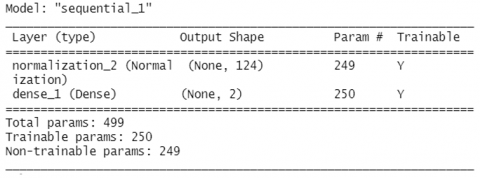
As seen in Table 2, each survey variable introduces different dispersion and distribution; therefore, a first normalization input layer adjusted to data behavior was designed in such a way that allows the neural network to use data on similar scales avoiding affectation effects on the gradients scale used in the training process. This normalization layer was implemented using the layer_normalization and adapt functions of Keras. Additionally, the response variable was coded in Dummy format, through which two neurons were designed for the output layer capable of delivering the probability whether the farm is prone to the appearance of Brucellosis, respectively. This encoding was done using the to_categorical function of Keras.
Next, an artificial neural network classification model without hidden layers was developed as a first neural approximation, consisting only of the normalization layer and two neurons in the output layer. The model was trained for 372 learning stages using Stochastic Gradient Descent (SGD) optimization, with Momentum set to 0.8 a learning rate decay starting at 0.1 and decreasing at 0.1/372 in each new learning stage. Three hundred seventy-two learning stages were selected following the rule of thumb [26], using triple the number of variables as learning stages. The learning process results are presented in Figure 1, and the architecture of the classifier is presented in Figure 2.
The classifier designed with two neurons in the output layer, without hidden layers, was evaluated in the 30% observations test set, corresponding to 192 observations unidentified by the classifier. Through these new observations, the classifier performance was evaluated, incicating a 5.6826267 loss, 0.8593750 accuracy, and 0.1210219 MSE obtained.
3.3 Establishing neural network topology
As seen in the classifier results Figure 2, performance metrics are still considerably far from optimal performance, so a set of models of Shallow Neural Networks and Deep Neural Networks was proposed, aiming to improve classifier performance. Thus, a technique for determining the optimal topology of the neural network was used, consisting of principal component analysis (PCA) to calculating the neural network optimal number of hidden layers [20, 21] and the exploration of all possible configurations in the neurons number of hidden layers following the recommendations [26].
As a dimension reduction technique, PCA makes it possible to determine the number of variables by which the variance in a group of variables can be progressively explained.
The PCA was executed using the princomp function of R; results are seen in Table 3 and Figure 3.
As shown in Figure 3, more than three main components are required in the model to explain more than 70% variance from observed data. For this reason, according to the studies [20, 21], models with up to 4 hidden layers were proposed to determine the topology of the neural network.
Figure 2. Training process of the two-neuron classifier without hidden layers
Table 3. Results of the principal component analysis executed on the database
|
Components |
Comp.1 |
Comp.2 |
Comp.3 |
Comp.4 |
Comp.5 |
|
Standard deviation |
0.5094 |
0.4464 |
0.3551 |
0.24470 |
0.1525 |
|
Proportion of variance |
0.3884 |
0.2983 |
0.1887 |
0.08961 |
0.0348 |
|
Cumulative ratio |
0.3884 |
0.6867 |
0.8755 |
0.96515 |
1,0000 |
Figure 3. Two-neuron classifier architecture without hidden layers
3.4 One hidden layer shallow neural network
Next, the optimal number of neurons was determined for the shallow neural network model with a single hidden layer. An iterative loop was designed to train various networks using different configurations, storing parameters and performance metrics.
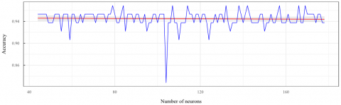
For the first hidden layer, activation function relu was used, with L2 regularization using a penalty parameter of L=0.01 to reduce parameter value preventing overfitting problems when adding neurons. Like the previous classifier, the SGD optimizer was used in this model with a 0.1 learning rate, a 0.8 Momentum, and a 0.0002688 learning-rate decay. For the first hidden layer selection of the number of neurons, all the possible configurations of neurons were implemented, from a minimum of half to a maximum of double the neurons in the input layer, in this case, 62 to 248 neurons since there were 124 entries for the hidden layer. The results of the performance metrics evaluated for each neuron first hidden layer configuration detailed in Table 4 and Figure 4.
As seen in Table 4 and Figure 4, when testing all the configurations for the neural network first hidden layer number of neurons, it was determined that there are configurations with considerably higher performance. In particular, configurations of 79, 80, 89, and 158 neurons can be highlighted, reaching Loss values in validations 0.688, 0.692, 0.349, and 0.598, respectively, suggesting that any of would be an optimal configuration. However, 89-neuron configuration reaching the best metrics in the experiments was selected. In addition, in Figure 4, the number of neurons in the hidden layer increase as the Loss values generally increase, while the Accuracy increases and the MSE decreases, suggesting that increasing the number of neurons does not always improve the model. The training process and architecture of the neural network with a proposed hidden layer are presented in Figures 5 and 6.
Figure 4. Cumulative variance proportion for each number of components obtained through PCA
Table 4. Performance metrics for different neural network configurations with a single hidden layer
|
Number of Neurons |
Loss |
Accuracy |
MSE |
Number of Neurons |
Loss |
Accuracy |
MSE |
Number of Neurons |
Loss |
Accuracy |
MSE |
|
62 |
2.4104 |
0.9531 |
0.0527 |
125 |
31.6380 |
0.9219 |
0.0662 |
188 |
14.6382 |
0.9688 |
0.0313 |
|
63 |
8.2155 |
0.9375 |
0.0517 |
126 |
24.3822 |
0.9375 |
0.0612 |
189 |
2.1478 |
0.9531 |
0.0385 |
|
64 |
11.4289 |
0.9219 |
0.0659 |
127 |
1.1792 |
0.9375 |
0.0462 |
190 |
14.8598 |
0.9375 |
0.0625 |
|
65 |
1.9282 |
0.9375 |
0.0577 |
128 |
4.2055 |
0.9531 |
0.0471 |
191 |
36.6496 |
0.9375 |
0.0576 |
|
66 |
7.8743 |
0.9219 |
0.0752 |
129 |
7.8582 |
0.9531 |
0.0436 |
192 |
16.0786 |
0.9375 |
0.0514 |
|
67 |
7.9107 |
0.9219 |
0.0631 |
130 |
16.3690 |
0.9219 |
0.0656 |
193 |
19.2104 |
0.9531 |
0.0320 |
|
68 |
2.5824 |
0.9219 |
0.0689 |
131 |
0.7084 |
0.9688 |
0.0235 |
194 |
8.8482 |
0.9375 |
0.0508 |
|
69 |
2.1165 |
0.9531 |
0.0510 |
132 |
42.7086 |
0.9375 |
0.0648 |
195 |
27.9806 |
0.9531 |
0.0446 |
|
70 |
4.2298 |
0.9531 |
0.0499 |
133 |
5.3914 |
0.9375 |
0.0555 |
196 |
11.8391 |
0.9375 |
0.0680 |
|
71 |
9.2280 |
0.9063 |
0.0590 |
134 |
9.9933 |
0.9531 |
0.0380 |
197 |
12.9974 |
0.9375 |
0.0556 |
|
72 |
3.4622 |
0.9531 |
0.0424 |
135 |
6.4385 |
0.9688 |
0.0305 |
198 |
10.3186 |
0.9219 |
0.0573 |
|
73 |
3.8671 |
0.9219 |
0.0781 |
136 |
26.2902 |
0.9531 |
0.0468 |
199 |
5.4273 |
0.9531 |
0.0443 |
|
74 |
7.3284 |
0.9688 |
0.0247 |
137 |
2.6988 |
0.9688 |
0.0261 |
200 |
10.4735 |
0.9375 |
0.0560 |
|
75 |
4.2898 |
0.9063 |
0.0796 |
138 |
4.7024 |
0.9688 |
0.0304 |
201 |
18.0530 |
0.9219 |
0.0723 |
|
76 |
21.9443 |
0.9063 |
0.0716 |
139 |
24.8153 |
0.9219 |
0.0817 |
202 |
0.8184 |
0.9531 |
0.0462 |
|
77 |
3.4176 |
0.9375 |
0.0502 |
140 |
1.2902 |
0.9375 |
0.0397 |
203 |
5.3224 |
0.9531 |
0.0401 |
|
78 |
30.4339 |
0.9219 |
0.0585 |
141 |
8.4655 |
0.9531 |
0.0320 |
204 |
2.1262 |
0.9531 |
0.0365 |
|
79 |
0.6890 |
0.9375 |
0.0487 |
142 |
14.0751 |
0.9219 |
0.0733 |
205 |
21.3395 |
0.9531 |
0.0397 |
|
80 |
0.6922 |
0.8906 |
0.0555 |
143 |
18.5304 |
0.9531 |
0.0395 |
206 |
11.1953 |
0.9531 |
0.0469 |
|
81 |
11.6949 |
0.9219 |
0.0607 |
144 |
5.3338 |
0.9375 |
0.0614 |
207 |
1.6601 |
0.9375 |
0.0458 |
|
82 |
0.8093 |
0.9531 |
0.0477 |
145 |
13.9484 |
0.9375 |
0.0509 |
208 |
5.9637 |
0.9375 |
0.0477 |
|
83 |
2.0386 |
0.9375 |
0.0425 |
146 |
19.9955 |
0.9531 |
0.0278 |
209 |
8.6627 |
0.9688 |
0.0312 |
|
84 |
8.5365 |
0.9375 |
0.0576 |
147 |
13.0036 |
0.9375 |
0.0610 |
210 |
41.2424 |
0.9375 |
0.0661 |
|
85 |
3.0151 |
0.9375 |
0.0560 |
148 |
12.5357 |
0.9375 |
0.0532 |
211 |
25.2603 |
0.9219 |
0.0679 |
|
86 |
2.1296 |
0.9375 |
0.0427 |
149 |
18.5093 |
0.9219 |
0.0653 |
212 |
5.0725 |
0.9531 |
0.0401 |
|
87 |
8.4835 |
0.9531 |
0.0460 |
150 |
12.9038 |
0.9375 |
0.0462 |
213 |
9.3957 |
0.9375 |
0.0571 |
|
88 |
1.5523 |
0.9375 |
0.0463 |
151 |
9.0566 |
0.9375 |
0.0474 |
214 |
12.2781 |
0.9063 |
0.0608 |
|
89 |
0.3495 |
0.9375 |
0.0461 |
152 |
20.3139 |
0.9219 |
0.0705 |
215 |
11.1058 |
0.9531 |
0.0428 |
|
90 |
2.7658 |
0.9375 |
0.0525 |
153 |
14.0581 |
0.9063 |
0.0737 |
216 |
7.7778 |
0.9531 |
0.0404 |
|
91 |
5.3761 |
0.9531 |
0.0345 |
154 |
6.5355 |
0.9375 |
0.0538 |
217 |
31.8098 |
0.9375 |
0.0549 |
|
92 |
2.0979 |
0.9531 |
0.0448 |
155 |
1.7559 |
0.9375 |
0.0567 |
218 |
0.7161 |
0.9531 |
0.0419 |
|
93 |
9.5000 |
0.9375 |
0.0453 |
156 |
8.3168 |
0.9531 |
0.0426 |
219 |
11.0355 |
0.8906 |
0.0708 |
|
94 |
0.9192 |
0.9375 |
0.0321 |
157 |
4.7196 |
0.9219 |
0.0678 |
220 |
7.1842 |
0.9375 |
0.0437 |
|
95 |
1.7273 |
0.9375 |
0.0509 |
158 |
0.5980 |
0.9531 |
0.0313 |
221 |
8.3809 |
0.9531 |
0.0399 |
|
96 |
10.8275 |
0.9375 |
0.0557 |
159 |
20.5459 |
0.9375 |
0.0605 |
222 |
53.9297 |
0.9531 |
0.0406 |
|
97 |
6.0879 |
0.9375 |
0.0470 |
160 |
2.2431 |
0.9531 |
0.0403 |
223 |
7.1866 |
0.9375 |
0.0593 |
|
98 |
2.0375 |
0.9531 |
0.0417 |
161 |
7.6714 |
0.9375 |
0.0563 |
224 |
18.9589 |
0.9375 |
0.0488 |
|
99 |
4.5898 |
0.9219 |
0.0573 |
162 |
3.6023 |
0.9375 |
0.0639 |
225 |
115.4788 |
0.8750 |
0.0930 |
|
100 |
8.1701 |
0.9375 |
0.0397 |
163 |
3.5185 |
0.9531 |
0.0479 |
226 |
34.6113 |
0.9688 |
0.0313 |
|
101 |
2.8501 |
0.9375 |
0.0456 |
164 |
5.6572 |
0.9531 |
0.0434 |
227 |
5.9036 |
0.9375 |
0.0513 |
|
102 |
2.8431 |
0.8906 |
0.0740 |
165 |
7.3310 |
0.9375 |
0.0583 |
228 |
3.5541 |
0.9375 |
0.0662 |
|
103 |
23.8387 |
0.9375 |
0.0525 |
166 |
10.5446 |
0.9219 |
0.0568 |
229 |
32.0479 |
0.9531 |
0.0368 |
|
104 |
1.4773 |
0.9219 |
0.0611 |
167 |
14.1403 |
0.9531 |
0.0455 |
230 |
2.0574 |
0.9375 |
0.0548 |
|
105 |
0.8356 |
0.9531 |
0.0544 |
168 |
16.6624 |
0.9531 |
0.0341 |
231 |
43.2719 |
0.9375 |
0.0475 |
|
106 |
3.0973 |
0.9375 |
0.0551 |
169 |
2.7685 |
0.9688 |
0.0323 |
232 |
35.8593 |
0.9375 |
0.0550 |
|
107 |
3.2981 |
0.9375 |
0.0470 |
170 |
13.2495 |
0.9375 |
0.0503 |
233 |
3.5197 |
0.9531 |
0.0415 |
|
108 |
16.6581 |
0.9219 |
0.0777 |
171 |
20.0442 |
0.9219 |
0.0704 |
234 |
19.2165 |
0.9531 |
0.0356 |
|
109 |
4.7416 |
0.9531 |
0.0499 |
172 |
21.9880 |
0.9375 |
0.0572 |
235 |
41.1777 |
0.9688 |
0.0313 |
|
110 |
2.8413 |
0.9375 |
0.0589 |
173 |
1.7927 |
0.9531 |
0.0315 |
236 |
9.4484 |
0.9688 |
0.0344 |
|
111 |
18.8791 |
0.9375 |
0.0559 |
174 |
89.9920 |
0.9063 |
0.0860 |
237 |
52.9232 |
0.9219 |
0.0663 |
|
112 |
2.3230 |
0.9531 |
0.0424 |
175 |
16.4002 |
0.9375 |
0.0482 |
238 |
18.1829 |
0.9375 |
0.0553 |
|
113 |
1.5639 |
0.9375 |
0.0580 |
176 |
14.9740 |
0.9531 |
0.0485 |
239 |
5.3080 |
0.9375 |
0.0500 |
|
114 |
0.1114 |
0.9531 |
0.0373 |
177 |
11.6100 |
0.9531 |
0.0328 |
240 |
7.1684 |
0.9219 |
0.0641 |
|
115 |
9.2677 |
0.9688 |
0.0235 |
178 |
13.0627 |
0.9375 |
0.0444 |
241 |
13.6392 |
0.9375 |
0.0527 |
|
116 |
5.9265 |
0.9375 |
0.0552 |
179 |
6.5480 |
0.9531 |
0.0298 |
242 |
6.2603 |
0.9219 |
0.0656 |
|
117 |
3.4074 |
0.9219 |
0.0602 |
180 |
1.4833 |
0.9375 |
0.0538 |
243 |
23.9679 |
0.9219 |
0.0749 |
|
118 |
3.0353 |
0.9531 |
0.0418 |
181 |
14.2464 |
0.9063 |
0.0690 |
244 |
1.7815 |
0.9531 |
0.0434 |
|
119 |
4.3757 |
0.9531 |
0.0571 |
182 |
24.2594 |
0.9688 |
0.0312 |
245 |
7.4158 |
0.9531 |
0.0507 |
|
120 |
11.8774 |
0.9219 |
0.0715 |
183 |
0.9693 |
0.9688 |
0.0282 |
246 |
23.4501 |
0.9531 |
0.0437 |
|
121 |
13.4641 |
0.9375 |
0.0569 |
184 |
11.5548 |
0.9531 |
0.0486 |
247 |
4.5637 |
0.9531 |
0.0452 |
|
122 |
1.2233 |
0.9531 |
0.0446 |
185 |
1.3170 |
0.9688 |
0.0319 |
248 |
0.7573 |
0.9688 |
0.0343 |
|
123 |
35.4805 |
0.9375 |
0.0528 |
186 |
19.2447 |
0.9688 |
0.0277 |
|
|
|
|
|
124 |
1.7569 |
0.9531 |
0.0409 |
187 |
11.8491 |
0.9375 |
0.0663 |
|
|
|
|
3.5 Deep learning models
Next, as detailed in Table 3, at least three hidden layers are the suggested number of hidden layers and components required to explain variable cumulative variance comprising the survey. That is why we explored the possible number of neurons configurations for each hidden layer. We built and trained a model for each hidden layer from half to twice the number of input neurons from previous layer that works as input for each hidden layer [26]. This allowed the testing of each configuration possible and select the most suitable number of neurons for each hidden layer based on performance metrics saving its parameters to be retrained in the next stage, adding an extra hidden layer. This process was repeated from two to four hidden layers.
As the first step for exploring the deep learning alternatives, a second hidden layer was added to verify if there were performance improvements compared to previous configurations. For the next hidden layer, the most neuron number configurations were tried, from half to double the neurons of the previous layer. As the first hidden layer was designed with 89 neurons, combinations from 44 to 178 neurons were tested in the second layer. Again, the neurons were implemented using the relu activation function, with L2 regularization setting its parameter in L=0.001, and SGD performed the optimization with a 0.8 moment and a 0.0002688 Learning- decay rate. Next, the above process was repeated to determine the optimal configuration of neurons in the third hidden layer. Next, each model was evaluated from 39 to 158 neurons for the third hidden layer, thus considering from half to double the neurons of the previous layer. Once again, neurons were configured with relu activation function, L2 regularization, 0.8 Momentum, and a 0.0002688 learning-rate decay to prevent overfitting. Finally, the greatest configuration for a neural network model with four hidden layers was determined. Similarly, every possible configuration from 23 to 94 neurons was tested. Like the previous ones, the fourth hidden layer was configured with the same hyperparameter configuration of the previous hidden layers.
The results for Loss, Accuracy, and MSE metrics in each configuration, number of neurons hidden layers used in the second, third, and fourth hidden layers, are presented in Table 5 and Figure 7.
As can be seen in Table 5, in the second hidden layer section, there were several configurations in the optimal number of neurons that achieve excellent performance metrics, highlighting neuron configurations 79, 100, 142, 156, and 164 reaching 0.1356, 0.1697, 0.1383, 0.1509 and 0.1375 Loss values respectively. Additionally, the configuration of 79 neurons was selected for the second hidden layer since, even though it reached a slightly lower MSE than the configuration of 142 neurons, it has a lower Loss metric and a similar Accuracy value. Moreover, as seen in the third hidden layer section (Table 5), some neural network configurations presented paramount performance, as configurations of 47 and 137 neurons stand out, reaching a 0.1341 and 0.1979 Loss respectively. In this way, the configuration of 47 neurons was selected since it reached a Loss lower than the models with two hidden layers and improved the accuracy reaching 97.31%.
Figure 5. Loss, Accuracy, and MSE for each neuron configuration implemented for the first hidden layer of the neural network
Table 5. Performance metrics for the trained and tested deep learning configurations with two, three, and four hidden layers
|
Two Hidden Layers Deep Learning Models |
|||||||||||||||||||||||||||||||
|
Number of Neurons |
Loss |
Accuracy |
MSE |
Number of Neurons |
Loss |
Accuracy |
MSE |
Number of Neurons |
Loss |
Accuracy |
MSE |
||||||||||||||||||||
|
44 |
0.2504 |
0.9531 |
0.0425 |
89 |
0.2761 |
0.9375 |
0.0528 |
134 |
0.2553 |
0.9219 |
0.0521 |
||||||||||||||||||||
|
45 |
0.1736 |
0.9531 |
0.0307 |
90 |
0.3328 |
0.9531 |
0.0462 |
135 |
0.3243 |
0.9375 |
0.0413 |
||||||||||||||||||||
|
46 |
0.2025 |
0.9531 |
0.0455 |
91 |
0.2401 |
0.9531 |
0.0465 |
136 |
0.2544 |
0.9375 |
0.0474 |
||||||||||||||||||||
|
47 |
0.2303 |
0.9531 |
0.0421 |
92 |
0.3380 |
0.9375 |
0.0582 |
137 |
0.2277 |
0.9375 |
0.0483 |
||||||||||||||||||||
|
48 |
0.2533 |
0.9531 |
0.0393 |
93 |
0.2738 |
0.9375 |
0.0548 |
138 |
0.2744 |
0.9688 |
0.0335 |
||||||||||||||||||||
|
49 |
0.3527 |
0.9375 |
0.0509 |
94 |
0.2700 |
0.9531 |
0.0399 |
139 |
0.3113 |
0.9531 |
0.0435 |
||||||||||||||||||||
|
50 |
0.1939 |
0.9375 |
0.0465 |
95 |
0.4145 |
0.9219 |
0.0674 |
140 |
0.3145 |
0.9375 |
0.0571 |
||||||||||||||||||||
|
51 |
0.2652 |
0.9375 |
0.0560 |
96 |
0.2674 |
0.9375 |
0.0590 |
141 |
0.2324 |
0.9531 |
0.0445 |
||||||||||||||||||||
|
52 |
0.2189 |
0.9531 |
0.0475 |
97 |
0.3774 |
0.9375 |
0.0532 |
142 |
0.1384 |
0.9688 |
0.0285 |
||||||||||||||||||||
|
53 |
0.3042 |
0.9531 |
0.0472 |
98 |
0.2193 |
0.9531 |
0.0361 |
143 |
0.2223 |
0.9531 |
0.0461 |
||||||||||||||||||||
|
54 |
0.3158 |
0.9531 |
0.0472 |
99 |
0.2105 |
0.9531 |
0.0376 |
144 |
0.2748 |
0.9375 |
0.0519 |
||||||||||||||||||||
|
55 |
0.3162 |
0.9219 |
0.0605 |
100 |
0.1698 |
0.9375 |
0.0414 |
145 |
0.3376 |
0.9375 |
0.0564 |
||||||||||||||||||||
|
56 |
0.2103 |
0.9531 |
0.0451 |
101 |
0.2273 |
0.9531 |
0.0359 |
146 |
0.2431 |
0.9375 |
0.0484 |
||||||||||||||||||||
|
57 |
0.2120 |
0.9531 |
0.0412 |
102 |
0.2016 |
0.9531 |
0.0357 |
147 |
0.2376 |
0.9375 |
0.0428 |
||||||||||||||||||||
|
58 |
0.2108 |
0.9531 |
0.0400 |
103 |
0.3204 |
0.9531 |
0.0410 |
148 |
0.3038 |
0.9531 |
0.0469 |
||||||||||||||||||||
|
59 |
0.3038 |
0.9063 |
0.0782 |
104 |
0.4358 |
0.8281 |
0.1168 |
149 |
0.1766 |
0.9531 |
0.0394 |
||||||||||||||||||||
|
60 |
0.2907 |
0.9531 |
0.0453 |
105 |
0.2164 |
0.9375 |
0.0486 |
150 |
0.2784 |
0.9219 |
0.0595 |
||||||||||||||||||||
|
61 |
0.2374 |
0.9531 |
0.0382 |
106 |
0.2545 |
0.9375 |
0.0517 |
151 |
0.4559 |
0.9375 |
0.0533 |
||||||||||||||||||||
|
62 |
0.2937 |
0.9375 |
0.0527 |
107 |
0.1987 |
0.9688 |
0.0328 |
152 |
0.2198 |
0.9375 |
0.0458 |
||||||||||||||||||||
|
63 |
0.3129 |
0.9375 |
0.0526 |
108 |
0.2385 |
0.9375 |
0.0505 |
153 |
0.2817 |
0.9531 |
0.0434 |
||||||||||||||||||||
|
64 |
0.2404 |
0.9531 |
0.0408 |
109 |
0.2447 |
0.9375 |
0.0517 |
154 |
0.2016 |
0.9375 |
0.0439 |
||||||||||||||||||||
|
65 |
0.2803 |
0.9375 |
0.0502 |
110 |
0.2396 |
0.9063 |
0.0533 |
155 |
0.2040 |
0.9375 |
0.0516 |
||||||||||||||||||||
|
66 |
0.2449 |
0.9531 |
0.0514 |
111 |
0.2354 |
0.9375 |
0.0498 |
156 |
0.1510 |
0.9531 |
0.0358 |
||||||||||||||||||||
|
67 |
0.3330 |
0.9531 |
0.0436 |
112 |
0.3918 |
0.9375 |
0.0554 |
157 |
0.1923 |
0.9688 |
0.0357 |
||||||||||||||||||||
|
68 |
0.1696 |
0.9531 |
0.0368 |
113 |
0.2591 |
0.9375 |
0.0491 |
158 |
0.2853 |
0.9375 |
0.0491 |
||||||||||||||||||||
|
69 |
0.2797 |
0.9531 |
0.0423 |
114 |
0.2739 |
0.9688 |
0.0365 |
159 |
0.3110 |
0.9375 |
0.0508 |
||||||||||||||||||||
|
70 |
0.2435 |
0.9531 |
0.0440 |
115 |
0.3307 |
0.9531 |
0.0477 |
160 |
0.2252 |
0.9375 |
0.0537 |
||||||||||||||||||||
|
71 |
0.4768 |
0.9375 |
0.0526 |
116 |
0.2076 |
0.9531 |
0.0395 |
161 |
0.2867 |
0.9531 |
0.0376 |
||||||||||||||||||||
|
72 |
0.2663 |
0.9531 |
0.0389 |
117 |
0.2806 |
0.9375 |
0.0500 |
162 |
0.2932 |
0.9375 |
0.0509 |
||||||||||||||||||||
|
73 |
0.2692 |
0.9531 |
0.0382 |
118 |
0.1995 |
0.9531 |
0.0348 |
163 |
0.3001 |
0.9375 |
0.0494 |
||||||||||||||||||||
|
74 |
0.3182 |
0.9531 |
0.0443 |
119 |
0.2140 |
0.9531 |
0.0435 |
164 |
0.1376 |
0.9375 |
0.0409 |
||||||||||||||||||||
|
75 |
0.2686 |
0.9531 |
0.0463 |
120 |
0.2331 |
0.9375 |
0.0529 |
165 |
0.3835 |
0.9375 |
0.0530 |
||||||||||||||||||||
|
76 |
0.1702 |
0.9375 |
0.0420 |
121 |
0.2612 |
0.9531 |
0.0390 |
166 |
0.2373 |
0.9688 |
0.0386 |
||||||||||||||||||||
|
77 |
0.2394 |
0.9531 |
0.0387 |
122 |
0.1968 |
0.9531 |
0.0425 |
167 |
0.2964 |
0.9375 |
0.0485 |
||||||||||||||||||||
|
78 |
0.2668 |
0.9531 |
0.0394 |
123 |
0.2185 |
0.9375 |
0.0481 |
168 |
0.2429 |
0.9375 |
0.0463 |
||||||||||||||||||||
|
79 |
0.1357 |
0.9688 |
0.0287 |
124 |
0.4783 |
0.9063 |
0.0919 |
169 |
0.3149 |
0.9688 |
0.0351 |
||||||||||||||||||||
|
80 |
0.3250 |
0.9531 |
0.0417 |
125 |
0.3513 |
0.9375 |
0.0590 |
170 |
0.2503 |
0.9531 |
0.0468 |
||||||||||||||||||||
|
81 |
0.2489 |
0.9375 |
0.0486 |
126 |
0.3121 |
0.9375 |
0.0514 |
171 |
0.2307 |
0.9531 |
0.0413 |
||||||||||||||||||||
|
82 |
0.3821 |
0.9375 |
0.0609 |
127 |
0.2183 |
0.9531 |
0.0396 |
172 |
0.2382 |
0.9531 |
0.0411 |
||||||||||||||||||||
|
83 |
0.2121 |
0.9531 |
0.0353 |
128 |
0.2211 |
0.9375 |
0.0455 |
173 |
0.2923 |
0.9531 |
0.0407 |
||||||||||||||||||||
|
84 |
0.2070 |
0.9688 |
0.0366 |
129 |
0.2870 |
0.9531 |
0.0440 |
174 |
0.4472 |
0.9375 |
0.0550 |
||||||||||||||||||||
|
85 |
0.2339 |
0.9219 |
0.0548 |
130 |
0.2201 |
0.9531 |
0.0376 |
175 |
0.2326 |
0.9531 |
0.0393 |
||||||||||||||||||||
|
86 |
0.2887 |
0.9531 |
0.0498 |
131 |
0.2411 |
0.9375 |
0.0583 |
176 |
0.2595 |
0.9531 |
0.0394 |
||||||||||||||||||||
|
87 |
0.2519 |
0.9531 |
0.0427 |
132 |
0.3420 |
0.9688 |
0.0354 |
177 |
0.2536 |
0.9375 |
0.0496 |
||||||||||||||||||||
|
88 |
0.1924 |
0.9531 |
0.0368 |
133 |
0.1965 |
0.9375 |
0.0459 |
178 |
0.2124 |
0.9375 |
0.0492 |
||||||||||||||||||||
|
Two Hidden Layers Deep Learning Models |
|||||||||||||||||||||||||||||||
|
Number of Neurons |
Loss |
Accuracy |
MSE |
Number of Neurons |
Loss |
Accuracy |
MSE |
Number of Neurons |
Loss |
Accuracy |
MSE |
||||||||||||||||||||
|
39 |
0.2712 |
0.9531 |
0.0463 |
79 |
0.3199 |
0.9375 |
0.0559 |
119 |
0.2646 |
0.9375 |
0.0527 |
||||||||||||||||||||
|
40 |
0.2913 |
0.9531 |
0.0421 |
80 |
0.3054 |
0.9375 |
0.0567 |
120 |
0.2734 |
0.9531 |
0.0427 |
||||||||||||||||||||
|
41 |
0.2852 |
0.9375 |
0.0561 |
81 |
0.4361 |
0.9531 |
0.0453 |
121 |
0.2560 |
0.9375 |
0.0522 |
||||||||||||||||||||
|
42 |
0.2022 |
0.9531 |
0.0407 |
82 |
0.3408 |
0.9375 |
0.0565 |
122 |
0.2105 |
0.9531 |
0.0412 |
||||||||||||||||||||
|
43 |
0.3129 |
0.9531 |
0.0455 |
83 |
0.2155 |
0.9531 |
0.0445 |
123 |
0.2258 |
0.9219 |
0.0538 |
||||||||||||||||||||
|
44 |
0.2501 |
0.9531 |
0.0421 |
84 |
0.2270 |
0.9531 |
0.0389 |
124 |
0.3114 |
0.9688 |
0.0303 |
||||||||||||||||||||
|
45 |
0.2857 |
0.9531 |
0.0490 |
85 |
0.1823 |
0.9375 |
0.0476 |
125 |
0.3024 |
0.9531 |
0.0401 |
||||||||||||||||||||
|
46 |
0.2727 |
0.9375 |
0.0497 |
86 |
0.3282 |
0.9531 |
0.0477 |
126 |
0.2778 |
0.9531 |
0.0482 |
||||||||||||||||||||
|
47 |
0.1342 |
0.9731 |
0.0278 |
87 |
0.2457 |
0.9531 |
0.0367 |
127 |
0.2433 |
0.9531 |
0.0476 |
||||||||||||||||||||
|
48 |
0.2533 |
0.9531 |
0.0448 |
88 |
0.2982 |
0.9375 |
0.0502 |
128 |
0.2293 |
0.9531 |
0.0378 |
||||||||||||||||||||
|
49 |
0.2393 |
0.9531 |
0.0421 |
89 |
0.2713 |
0.9375 |
0.0522 |
129 |
0.2442 |
0.9219 |
0.0558 |
||||||||||||||||||||
|
50 |
0.2467 |
0.9063 |
0.0716 |
90 |
0.2271 |
0.9375 |
0.0567 |
130 |
0.2480 |
0.9531 |
0.0465 |
||||||||||||||||||||
|
51 |
0.2343 |
0.9531 |
0.0444 |
91 |
0.2506 |
0.9375 |
0.0533 |
131 |
0.3499 |
0.9531 |
0.0517 |
||||||||||||||||||||
|
52 |
0.2166 |
0.9531 |
0.0420 |
92 |
0.2855 |
0.9375 |
0.0559 |
132 |
0.2429 |
0.9531 |
0.0435 |
||||||||||||||||||||
|
53 |
0.2626 |
0.9688 |
0.0328 |
93 |
0.2452 |
0.9531 |
0.0443 |
133 |
0.2469 |
0.9375 |
0.0495 |
||||||||||||||||||||
|
54 |
0.2094 |
0.9688 |
0.0300 |
94 |
0.2554 |
0.9531 |
0.0436 |
134 |
0.2629 |
0.9531 |
0.0468 |
||||||||||||||||||||
|
55 |
0.2325 |
0.9531 |
0.0429 |
95 |
0.3894 |
0.9375 |
0.0613 |
135 |
0.3022 |
0.9688 |
0.0353 |
||||||||||||||||||||
|
56 |
0.2619 |
0.9531 |
0.0398 |
96 |
0.2595 |
0.9531 |
0.0466 |
136 |
0.2346 |
0.9375 |
0.0573 |
||||||||||||||||||||
|
57 |
0.2717 |
0.9531 |
0.0455 |
97 |
0.3251 |
0.9688 |
0.0342 |
137 |
0.1979 |
0.9531 |
0.0447 |
||||||||||||||||||||
|
58 |
0.2010 |
0.9531 |
0.0382 |
98 |
0.2032 |
0.9688 |
0.0345 |
138 |
0.5476 |
0.8750 |
0.1110 |
||||||||||||||||||||
|
59 |
0.3305 |
0.9375 |
0.0541 |
99 |
0.2484 |
0.9688 |
0.0368 |
139 |
0.2814 |
0.8906 |
0.0684 |
||||||||||||||||||||
|
60 |
0.2695 |
0.9375 |
0.0483 |
100 |
0.2629 |
0.9531 |
0.0421 |
140 |
0.2759 |
0.9531 |
0.0382 |
||||||||||||||||||||
|
61 |
0.2652 |
0.9375 |
0.0498 |
101 |
0.2820 |
0.9531 |
0.0473 |
141 |
0.2156 |
0.9531 |
0.0395 |
||||||||||||||||||||
|
62 |
0.2596 |
0.9531 |
0.0425 |
102 |
0.2814 |
0.9375 |
0.0509 |
142 |
0.3642 |
0.9375 |
0.0608 |
||||||||||||||||||||
|
63 |
0.2332 |
0.9375 |
0.0459 |
103 |
0.2500 |
0.9531 |
0.0422 |
143 |
0.3446 |
0.9375 |
0.0589 |
||||||||||||||||||||
|
64 |
0.2407 |
0.9531 |
0.0480 |
104 |
0.2624 |
0.9531 |
0.0402 |
144 |
0.2088 |
0.9531 |
0.0450 |
||||||||||||||||||||
|
65 |
0.2404 |
0.9531 |
0.0435 |
105 |
0.1975 |
0.9375 |
0.0445 |
145 |
0.3554 |
0.9531 |
0.0470 |
||||||||||||||||||||
|
66 |
0.2675 |
0.9531 |
0.0434 |
106 |
0.2479 |
0.9531 |
0.0454 |
146 |
0.3366 |
0.9375 |
0.0477 |
||||||||||||||||||||
|
67 |
0.2851 |
0.9375 |
0.0490 |
107 |
0.3459 |
0.9375 |
0.0544 |
147 |
0.2275 |
0.9531 |
0.0442 |
||||||||||||||||||||
|
68 |
0.2416 |
0.9531 |
0.0458 |
108 |
0.1998 |
0.9531 |
0.0380 |
148 |
0.3414 |
0.9531 |
0.0477 |
||||||||||||||||||||
|
69 |
0.2300 |
0.9219 |
0.0590 |
109 |
0.2838 |
0.9531 |
0.0371 |
149 |
0.3709 |
0.9219 |
0.0655 |
||||||||||||||||||||
|
70 |
0.3210 |
0.9063 |
0.0858 |
110 |
0.2870 |
0.9531 |
0.0459 |
150 |
0.3630 |
0.9375 |
0.0560 |
||||||||||||||||||||
|
71 |
0.3781 |
0.9531 |
0.0432 |
111 |
0.2113 |
0.9531 |
0.0428 |
151 |
0.2738 |
0.9531 |
0.0384 |
||||||||||||||||||||
|
72 |
0.3385 |
0.9531 |
0.0500 |
112 |
0.4097 |
0.9375 |
0.0554 |
152 |
0.2799 |
0.9531 |
0.0434 |
||||||||||||||||||||
|
73 |
0.2265 |
0.9375 |
0.0452 |
113 |
0.2425 |
0.9531 |
0.0413 |
153 |
0.2711 |
0.9531 |
0.0428 |
||||||||||||||||||||
|
74 |
0.2193 |
0.9531 |
0.0446 |
114 |
0.3220 |
0.9375 |
0.0543 |
154 |
0.2343 |
0.9375 |
0.0565 |
||||||||||||||||||||
|
75 |
0.2263 |
0.9375 |
0.0439 |
115 |
0.2717 |
0.9531 |
0.0427 |
155 |
0.1652 |
0.9375 |
0.0428 |
||||||||||||||||||||
|
76 |
0.2899 |
0.9531 |
0.0472 |
116 |
0.3447 |
0.9375 |
0.0594 |
156 |
0.2628 |
0.9375 |
0.0517 |
||||||||||||||||||||
|
77 |
0.3606 |
0.9375 |
0.0605 |
117 |
0.2949 |
0.9531 |
0.0453 |
157 |
0.2921 |
0.9375 |
0.0508 |
||||||||||||||||||||
|
78 |
0.3187 |
0.9375 |
0.0524 |
118 |
0.2482 |
0.9375 |
0.0460 |
158 |
0.2542 |
0.9531 |
0.0382 |
||||||||||||||||||||
|
Four Hidden Layers Deep Learning Models |
|||||||||||||||||||||||||||||||
|
Number of Neurons |
Loss |
Accuracy |
MSE |
Number of Neurons |
Loss |
Accuracy |
MSE |
Number of Neurons |
Loss |
Accuracy |
MSE |
||||||||||||||||||||
|
23 |
0.2481 |
0.9219 |
0.0607 |
47 |
0.2469 |
0.9531 |
0.0411 |
71 |
0.2186 |
0.9531 |
0.0413 |
||||||||||||||||||||
|
24 |
0.2404 |
0.9531 |
0.0357 |
48 |
0.2885 |
0.9375 |
0.0587 |
72 |
0.2211 |
0.9531 |
0.0405 |
||||||||||||||||||||
|
25 |
0.3580 |
0.9531 |
0.0421 |
49 |
0.3135 |
0.9531 |
0.0470 |
73 |
0.2980 |
0.9531 |
0.0479 |
||||||||||||||||||||
|
26 |
0.2375 |
0.9531 |
0.0404 |
50 |
0.2861 |
0.9531 |
0.0493 |
74 |
0.2429 |
0.9531 |
0.0478 |
||||||||||||||||||||
|
27 |
0.2982 |
0.9375 |
0.0572 |
51 |
0.3948 |
0.9375 |
0.0564 |
75 |
0.2674 |
0.9531 |
0.0408 |
||||||||||||||||||||
|
28 |
0.2733 |
0.9531 |
0.0467 |
52 |
0.2847 |
0.9375 |
0.0567 |
76 |
0.2474 |
0.9531 |
0.0463 |
||||||||||||||||||||
|
29 |
0.2197 |
0.9531 |
0.0452 |
53 |
0.3263 |
0.9375 |
0.0590 |
77 |
0.2874 |
0.9375 |
0.0508 |
||||||||||||||||||||
|
30 |
0.3402 |
0.9531 |
0.0496 |
54 |
0.2895 |
0.9688 |
0.0337 |
78 |
0.3817 |
0.9375 |
0.0588 |
||||||||||||||||||||
|
31 |
0.2634 |
0.9531 |
0.0362 |
55 |
0.2300 |
0.9531 |
0.0451 |
79 |
0.2413 |
0.9531 |
0.0415 |
||||||||||||||||||||
|
32 |
0.2761 |
0.9531 |
0.0480 |
56 |
0.2671 |
0.9375 |
0.0423 |
80 |
0.3294 |
0.9375 |
0.0534 |
||||||||||||||||||||
|
33 |
0.2946 |
0.9531 |
0.0459 |
57 |
0.3036 |
0.9531 |
0.0464 |
81 |
0.2362 |
0.9375 |
0.0503 |
||||||||||||||||||||
|
34 |
0.3544 |
0.8750 |
0.0941 |
58 |
0.2618 |
0.9531 |
0.0386 |
82 |
0.2083 |
0.9531 |
0.0452 |
||||||||||||||||||||
|
35 |
0.3458 |
0.9531 |
0.0429 |
59 |
0.2410 |
0.9531 |
0.0464 |
83 |
0.2618 |
0.9531 |
0.0477 |
||||||||||||||||||||
|
36 |
0.1785 |
0.9531 |
0.0376 |
60 |
0.2506 |
0.9531 |
0.0395 |
84 |
0.3681 |
0.9375 |
0.0509 |
||||||||||||||||||||
|
37 |
0.2711 |
0.9531 |
0.0477 |
61 |
0.2818 |
0.9531 |
0.0452 |
85 |
0.3294 |
0.9531 |
0.0458 |
||||||||||||||||||||
|
38 |
0.2579 |
0.9375 |
0.0470 |
62 |
0.2870 |
0.9375 |
0.0480 |
86 |
0.2281 |
0.9531 |
0.0399 |
||||||||||||||||||||
|
39 |
0.2765 |
0.9531 |
0.0398 |
63 |
0.1873 |
0.9531 |
0.0415 |
87 |
0.2675 |
0.9375 |
0.0546 |
||||||||||||||||||||
|
40 |
0.4514 |
0.8594 |
0.1120 |
64 |
0.2596 |
0.9531 |
0.0440 |
88 |
0.2908 |
0.9375 |
0.0557 |
||||||||||||||||||||
|
41 |
0.2173 |
0.9375 |
0.0490 |
65 |
0.4345 |
0.9375 |
0.0617 |
89 |
0.2629 |
0.9531 |
0.0367 |
||||||||||||||||||||
|
42 |
0.3062 |
0.9531 |
0.0432 |
66 |
0.1935 |
0.9531 |
0.0454 |
90 |
0.3219 |
0.9375 |
0.0547 |
||||||||||||||||||||
|
43 |
0.2535 |
0.9531 |
0.0454 |
67 |
0.3061 |
0.9531 |
0.0425 |
91 |
0.2551 |
0.9531 |
0.0459 |
||||||||||||||||||||
|
44 |
0.4291 |
0.9531 |
0.0494 |
68 |
0.3439 |
0.9375 |
0.0569 |
92 |
0.2917 |
0.9531 |
0.0468 |
||||||||||||||||||||
|
45 |
0.2601 |
0.9531 |
0.0447 |
69 |
0.1644 |
0.9531 |
0.0381 |
93 |
0.4655 |
0.9219 |
0.0635 |
||||||||||||||||||||
|
46 |
0.3015 |
0.9531 |
0.0469 |
70 |
0.2374 |
0.9375 |
0.0578 |
94 |
0.2506 |
0.9531 |
0.0422 |
||||||||||||||||||||
Finally, in the fourth hidden layer section (Table 5), the outmost configuration for the number of neurons in the fourth layer was obtained using 36 neurons. However, compared with the training results of the models proposed for three hidden layers, it can be seen that the three hidden layer models achieved better Loss, Accuracy, and MSE metrics. An observed overfitting problem is highly noticeable determining that including more layers does not always mean improving metrics performance. This can be detected in the case of the fourth hidden layer, where its addition implied worsened metric performance, so we kept the three hidden layers model as the leading of the 324 trained and tested models.
Additionally, in Figure 8, through the projected trend lines for each metric, it can be seen that as the number of neurons increases, Loss and MSE increases, as accuracy decreases, suggesting that a greater number of neurons does not necessarily improve the model tending to present overfitting problems. This situation can be distinguised in the three rows Figure 8 being a common problem that occurred in hidden layers second, third, and fourth.
It must be pointed out that metrics presented in Table 5 and Figure 8 were obtained once the training process in each classifier ended, so the classifier was tested using dataset test obtained by splitting the entire dataset, as detailed in section 2.4.4. Consequenly the performance metrics presented as results were obtained using each model to classify 189 examples never seen before by the classifier during training.
As introduced in Table 5, the most advantageous deep learning architecture was the sequential model with a 89, 79, and 47 neurons configuration in its three hidden layers, corresponding to the outmost shallow neural network configuration retrained looking for the best architecture for the second hidden layer (achieved with 79 neurons) being retrained again adding a third hidden layer looking for optimal configuration (achieving 47 neurons). The training process ended in the fourth stage because none of the proposed four-hidden layers outperformed the best three-hidden layers model. The training process and the architecture of the most advantageous deep learning model in Figures 8-10.
In addition, topologies of the best models trained and tested for each hidden layer are provided in the annex section.
Finally, the performance of each proposed model was verified on the test data set that each model never observed during the training process [27]. The data set consisted of 64 observations for which the Loss, Accuracy, and MSE were obtained again. Results in Table 6.
Table 6. Implemented models comparison-evaluated on Test database
|
Models |
Loss |
Accuracy |
MSE |
|
Logistic regression |
7.75324 |
0.74521 |
0.24876 |
|
Classifier without hidden layers |
5.68262 |
0.85937 |
0.12102 |
|
Shallow neural network - one hidden layer |
0.26870 |
0.93750 |
0.05369 |
|
Two hidden layers sequential model |
0.10575 |
0.98437 |
0.01113 |
|
Three hidden layers sequential model |
0.03923 |
0.98437 |
0.00604 |
|
Four hidden layers sequential model |
0.05210 |
0.97875 |
0.00431 |
As seen in Table 6, the best-implemented model was the three hidden layers with 89, 79, and 47 neurons configuration, achieving 0.03923, 0.98437, and 0.00604 regarding Loss, Accuracy, and MSE metrics performance. This model was evaluated in greater detail using the confusion matrix and the ROC curve, achieving 0.984 Accuracy. Performance results of the Deep Learning classifier with three hidden layers are presented in Figures 6 and 7.
As observed in Figures 11 and 12, the best model among trained and tested proposals achieved 0.984 accuracy being by far the highest among all techniques. The accuracy considerably outperforms traditional methods like logistic regression achieving 0.74521accuracy, confirming the advantages of using deep learning techniques for classification based on non-linear datasets [28]. Additionally, precision and specificity were close to one, indicating a good confidence level on the true positive classifications and true negatives classification, respectively. The Recall of 0.982 suggests an exceptional level of prediction for the farms that presented Brucellosis risk. Also, given the different proportions that the true positives and false negatives presented in the test dataset, we looked at the F1 score, which achieved a 0.991 level placing this model as an optimal overall classifier. Finally, the observed 0.996 AUC represents an approving performance measurement at different threshold settings, confirming that the proposed model performance is satisfactorily enough to distinguish between farms at risk presenting Brucellosis risk.
Figure 6. Training process of the proposed one-hidden layer neural network
Figure 7. Architecture of the proposed one-hidden layer neural network
(a)
(b)
(c)
(d)
(e)
(f)
(g)
(h)
(i)
Figure 8. Loss, Accuracy, and MSE for each neuron configuration implemented for the second, third, and fourth hidden layers of the neural network
Note: The first row corresponds to (a) accuracy, (b) loss, and (c) MSE of every configuration trained for the second hidden layer. The second row corresponds to (d) accuracy, (e) loss, and (f) MSE of every trained configuration for the third hidden layer. Finally, the third row corresponds to (g) accuracy, (h) loss, and (i) MSE every trained configuration for the third hidden layer
Figure 9. Optimal training process for the proposed three-hidden-layer neural network
Figure 10. Best proposed architecture for three-hidden-layer neural network
Figure 11. Three hidden layers deep learning classifier confusion matrix
Figure 12. ROC curve for the deep learning classifier with three hidden layers
Through the exposed results, it is possible to visualize various multivariate techniques proposed in the literature analyzing categorical variables [23]. However, due to the binary coding given to the variables and the large number of variables considered (51 categorical variables equivalent to 125 dummy variables) conventional techniques such as decision trees and multiple and logistic regressions are not robust enough to obtain adequate models from this data. In contrast, neural networks ensembles artificial neurons, where each neuron can learn non-linear behaviors from the data. For this reason, as seen in Table 6 neural networks, especially the Deep Learning models reached superior performance levels and precision detecting on the spot Brucellosis risk in cattle farms. The three hidden layer model achieved 98.4% accuracy and 98.2%, sensitivity rivaling laboratory test results, demonstrating current artificial intelligence highly-powered techniques for tasks analyzing. The considerably better performance observed in the Deep Learning models can be mainly attributed to the non-linear variables comprising the survey. Similarly, it can also be attributed to factors like data complexity and the high number of variables considered as Brucellosis risk factors, indicated in Table 2. Also, comparing classic methods like Logistic regression, which only relies on one activation function, neural networks models present the advantage of using more than one activation function, which can be trained using different input variables subsets, pattern discovery and combinations of activations to propagate the information improving the classification task. For example, the top model presented three layers using 215 trained neurons, combining different sets of variable input in multiple stages so shat the model finds the most effective way to combine activations. Also, it must be mentioned that ML techniques have considerably evolved in recent years, at designing neural networks. In this particular case, we observed that the incorporating of normalization and regularization techniques significantly improved tested models performance. So, due to the complexity of the data used in this problem, the addition of normalization and regularization, an appropriate selection of the optimizer, activation, and loss functions, where the key factors that allowed the best three hidden layer model to achieve metrics high-performance in line to what was expected in the early PCA analysis.
An additional advantage implicit in this proposal is that the proposed diagnostic mechanism aims to be non-invasive and almost free since it does not require any people or animals’ intervention because the survey instrument only requires information already available in most farms in the Carchi province. Still, the variables in the survey considered levels to deal with information that does not apply to some farms. This configuration allowed the survey to be applied in 632 farms with minimum equipment (a smartphone or laptop) and minimum knowledge required by the interviewers visiting each farm gathering the required information in less than an hour per farm. The developed software was made publicly available for free download at https://github.com/erickherreraresearch/DeepBrucell; so its implementation and use in any farm in the Carchi province only requires a computer (commodity PC).
Unlike previous studies such as [9], where the diagnosis of Brucellosis is made in each animal using measurements based on DNA samples in combination with Deep Learning techniques, the technique proposed in this study can be applied without the need of laboratory samples using only categorical data representing risk factors widely identified in previous studies. As a result, it is possible to carry out an extremely precise diagnosis of Brucellosis risk in the farm but, limited to the generality of the farm that will allow the taking of general control actions. At the same time, the current method can be accompanied by laboratory tests identifying affected animals.
A limitation in this proposal is the veracity of data provided by respondents when the model is finally used. This drawback can be addressed in large databases like the one used for this study using data cleaning techniques such as Mahalanobis distances, Z-Score, and imputation techniques. But when applied to small datasets or punctual observations, the model’s precision could be severely affected by false information. Another limitation may be due to the absence of animal or herd physiological variables, considerably contributing to the improving of diagnosis accuracy and overcoming issues related to data veracity which will be a work field addressed in future projects out of the scope in this study. One last weak point is the overfitting frequently observed during training processes, resulting from variable complexity. Nevertheless, it is suggested that there could be risk factors not-included that promote a more exhaustive variable selection that make up the survey as it will be explored in future work.
To summarize, through an extensive experimentation, we compared multiple ML configurations to a classic classification technique to build an effective classifier for Brucellosis risk in farms based only on descriptive information about the farm and production system management. The leading model that outperformed the rest of tested configurations was the sequential Deep Learning model with 125 neuron input and three hidden layers in 89, 79, and 47 neurons configuration reaching a 0.98437 accuracy due to an appropriate topology selection and the use of normalization and regularization techniques highlighting the power of Deep Learning models in solving non-linear problems, even for complex multivariate data, where techniques like regressions and Shallow Neural Networks might become unsuitable.
In this study, a new Brucellosis risk detection method is proposed, applied to cattle farms at the Carchi province -Ecuador based on the gathering of risk factors information that has been widely identified in previous studies. The information required for the diagnosis was collected as an instrument made up of 51 categorical variables including farm location, farm general information, reproduction systems, reproductive pathologies, diagnosis, health control, milking, workers, and food consumption risk. Data from each farm were structured as observations in the designing of automatic classifiers developed used multivariate techniques. The classifiers considered for this study were logistic regression, neural classifiers without hidden layers, shallow neural networks, and various Deep Learning models.
Though an exhaustive experimental protocol, we conclude that Deep Learning models present a clear advantage over Shallow Neural Networks and classic techniques due to the non-linear nature of the risk factors proposed in the literature. Deep Learning models displayed the ability to capture risk factors non-linear behavior in optimum ways to combine information from these factors to produce an appropriate classification of Brucellosis risk on cattle farms, being crucial in this investigation due to data complexity and the large number of variables comprising the survey. Among all the techniques implemented, the 3 hidden layers model in 89, 79, and 47 neurons configuration achieved prime performance for the Brucellosis instant detection, reaching 98.437% accuracy, of 0.00604 MSE and 0.03923 Loss on a test database that was not observed by the classifier during training.
In this way, it can be concluded that it is possible to Diagnose the existence of Brucellosis in cattle farms from main risk factors identification accurately and reliably, through the use of Deep Learning techniques that in this study have proven to be the most suitable to model Brucellosis risk factors in the Carchi province, among the tested alternatives.
Constrains identified in this work were the veracity of the information provided by those surveyed, the absence of animal or herd physiological variables in the survey, and overfitting. These challenges will be addressed in future work, including animal physiological variables which would contribute to mitigating false information effects, and further selection of the new variables leading to a new set of more specific risk factors contributing to mitigating overfitting problems.
Video samples of each algorithm execution—indoors and outdoors is available as supplementary material in the GitHub repository: https://github.com/erickherreraresearch/DeepBrucell; along with all the .txt result files of each algorithm run for reproducibility.
Architecture of the best neural network models evaluated in this study presented in Figures A1-A5.
Figure A1. Architecture of the classifier with two neurons in the output layer, without hidden layers
Figure A2. Optimal neural network architecture determined configuration with one hidden layer (89 neurons)
Figure A3. Architecture of the best determined neural network configuration with two hidden layers (89 and 79 neurons)
Figure A4. Architecture of the best determined neural network configuration with three hidden layers (89, 79 and 47 neurons)
Figure A5. Architecture of the best determined neural network configuration with three hidden layers (89, 79, 47 and 36 neurons)
[1] Tulu, D. (2022). Bovine brucellosis: epidemiology, public health implications, and status of brucellosis in Ethiopia. Veterinary Medicine: Research and Reports, 13: 21-30. https://doi.org/10.2147/VMRR.S347337
[2] Rosero, E.M.I., Jiménez, R.E.S. (2016). Prevalencia de brucelosis (Brucella Abortus) y factores de riesgo en estudiantes de primero a noveno semestre de la escuela de Desarrollo Integral Agropecuario de la UPEC. Sathiri, 11: 303-313. https://doi.org/10.32645/13906925.28
[3] Chavisnan, G., Homero, P. (2018). Factores de riesgo asociados a la brucelosis bovina (Brucella abortus) en vacas en producción lechera en el cantón Montúfar (Doctoral dissertation, Universidad Politécnica Estatal del Carchi).
[4] Solera, J., Martinez-Alfaro, E., Espinosa, A., Castillejos, M.L., Geijo, P., Rodriguez-Zapata, M. (1998). Multivariate model for predicting relapse in human brucellosis. Journal of Infection, 36(1): 85-92. https://doi.org/10.1016/S0163-4453(98)93342-4
[5] Peng, C., Li, Y.J., Huang, D.S., Guan, P. (2020). Spatial-temporal distribution of human brucellosis in mainland China from 2004 to 2017 and an analysis of social and environmental factors. Environmental Health and Preventive Medicine, 25(1): 1-14. https://doi.org/10.1186/s12199-019-0839-z
[6] Khan, A.U., Melzer, F., Hendam, A., Sayour, A.E., Khan, I., Elschner, M.C., El-Adawy, H. (2020). Seroprevalence and Molecular Identification of Brucella spp. in Bovines in Pakistan—Investigating Association With Risk Factors Using Machine Learning. Frontiers in Veterinary Science, 7: 594498. https://doi.org/10.3389/fvets.2020.594498
[7] Djafar, Z.R., Benazi, N., Bounab, S., Sayhi, M., Diouani, M.F., Benia, F. (2020). Distribution of seroprevalence and risk factors for bovine tuberculosis in east Algeria. Preventive Veterinary Medicine, 183: 105127. https://doi.org/10.1016/j.prevetmed.2020.105127
[8] Ntivuguruzwa, J.B., Kolo, F.B., Gashururu, R.S., Umurerwa, L., Byaruhanga, C., Van Heerden, H. (2020). Seroprevalence and associated risk factors of bovine brucellosis at the wildlife-livestock-human interface in Rwanda. Microorganisms, 8(10): 1553. https://doi.org/10.3390/microorganisms8101553
[9] Sil, S., Mukherjee, R., Kumbhar, D., Reghu, D., Shrungar, D., Kumar, N.S., Umapathy, S. (2021). Raman spectroscopy and artificial intelligence open up accurate detection of pathogens from DNA-based sub-species level classification. Journal of Raman Spectroscopy, 52(12): 2648-2659. https://doi.org/10.1002/jrs.6115
[10] Saidu, A.S., Mahajan, N.K., Musallam, I.I., Holt, H.R., Guitian, J. (2021). Epidemiology of bovine brucellosis in Hisar, India: identification of risk factors and assessment of knowledge, attitudes, and practices among livestock owners. Tropical Animal Health and Production, 53: 1-12. https://doi.org/10.1007/s11250-021-02884-z
[11] Holt, H.R., Bedi, J.S., Kaur, P., Mangtani, P., Sharma, N.S., Gill, J.P.S., Guitian, J. (2021). Epidemiology of brucellosis in cattle and dairy farmers of rural Ludhiana, Punjab. PLoS Neglected Tropical Diseases, 15(3): e0009102. https://doi.org/10.1371/journal.pntd.0009102
[12] Abdel-Hamid, N.H., Ghobashy, H.M., Beleta, E.I., Elbauomy, E.M., Ismail, R.I., Nagati, S.F., Elmonir, W. (2021). Risk factors and Molecular genotyping of Brucella melitensis strains recovered from humans and their owned cattle in Upper Egypt. One Health, 13: 100281. https://doi.org/10.1016/j.onehlt.2021.100281
[13] Deka, R.P., Shome, R., Dohoo, I., Magnusson, U., Randolph, D.G., Lindahl, J.F. (2021). Seroprevalence and risk factors of Brucella infection in dairy animals in urban and rural areas of Bihar and Assam, India. Microorganisms, 9(4): 783. https://doi.org/10.3390/microorganisms9040783
[14] Etefa, M., Kabeta, T., Merga, D., Debelo, M. (2022). Cross-sectional study of seroprevalence and associated risk factors of bovine brucellosis in selected districts of Jimma zone, south western oromia, Ethiopia. BioMed Research International, 2022. https://doi.org/10.1155/2022/9549942
[15] Male Here, R.R., Ryan, E., Breslin, P., Frankena, K., Byrne, A.W. (2022). Revisiting the relative effectiveness of slaughterhouses in Ireland to detect tuberculosis lesions in cattle (2014–2018). Plos one, 17(10): e0275259. https://doi.org/10.1371/journal.pone.0275259
[16] Megahed, A., Kandeel, S., Alshaya, D.S., Attia, K.A., AlKahtani, M.D., Albohairy, F.M., Selim, A. (2022). A comparison of logistic regression and classification tree to assess brucellosis associated risk factors in dairy cattle. Preventive Veterinary Medicine, 203: 105664. https://doi.org/10.1016/j.prevetmed.2022.105664
[17] Ghorbani, H. (2019). Mahalanobis distance and its application for detecting multivariate outliers. Facta Universitatis, Series: Mathematics and Informatics, 583-595. https://doi.org/10.22190/FUMI1903583G
[18] Jácome Ortega, A.E., Caraguay Procel, J.A., Herrera-Granda, E.P., Herrera Granda, I.D. (2019). Confirmatory factorial analysis applied on teacher evaluation processes in higher education institutions of Ecuador. In International Conference on ‘Knowledge Society: Technology, Sustainability and Educational Innovation’, Ibarra, Ecuador, pp. 157-170. https://doi.org/10.1007/978-3-030-37221-7_14
[19] Reddy, G.T., Reddy, M.P.K., Lakshmanna, K., Kaluri, R., Rajput, D.S., Srivastava, G., Baker, T. (2020). Analysis of dimensionality reduction techniques on big data. Ieee Access, 8: 54776-54788. https://doi.org/10.1109/ACCESS.2020.2980942
[20] Ibnu Choldun R, M., Santoso, J., Surendro, K. (2020). Determining the number of hidden layers in neural network by using principal component analysis. In Intelligent Systems and Applications: Proceedings of the 2019 Intelligent Systems Conference (IntelliSys) Volume 2, London, United Kingdom, pp. 490-500. https://doi.org/10.1007/978-3-030-29513-4_36
[21] Rachmatullah, M.I.C., Santoso, J., Surendro, K. (2021). Determining the number of hidden layer and hidden neuron of neural network for wind speed prediction. PeerJ Computer Science, 7: e724. https://doi.org/10.7717/peerj-cs.724
[22] Weidman, S. (2019). Deep Learning from Scratch, First. Sebastopol: O’Reilly. https://www.oreilly.com/library/view/deep-learning-from/9781492041405
[23] Géron, A. (2019). Hands-On Machine Learning with Scikit-Learn, Keras, and TensorFlow, Second. Sebastopol: O’Reilly. https://www.oreilly.com/library/view/hands-on-machine-learning/9781492032632
[24] Tariq, R. (2017). Make Your Own Neural Network, First. CreateSpace Independent Publishing. http://makeyourownneuralnetwork.blogspot.co.uk
[25] Vujičić, T., Matijevi, T., Ljucović, J., Balota, A., Ševarac, Z. (2016). Comparative analysis of methods for determining number of hidden neurons in artificial neural network. In Central European conference on information and intelligent systems, Varaždin, Croatia, 219: 219-250.
[26] Demuth, H.B., Beale, M.H., De Jess, O., Hagan, M.T. (2014). Neural Network Design, 2nd ed. Stillwater, OK, USA: Martin Hagan. https://hagan.okstate.edu/NNDesign.pdf
[27] Herrera-Granda, E.P., Lorente-Leyva, L.L., Yambay, J., Aranguren, J., Ibarra, M., Peña, J. (2022). Controller modeling of a quadrotor. Ingénierie des Systèmes d’Information, 27(1): 21-28. https://doi.org/10.18280/isi.270103
[28] Arifin, M., Widowati, W., Farikhin, F. (2023). Optimization of hyperparameters in machine learning for enhancing predictions of student academic performance. Ingénierie des Systèmes d’Information, 28(3): 575-582. https://doi.org/10.18280/isi.280305