Zuhair Shakor Mhmood*![]() | Ali Najdet Nasret
| Ali Najdet Nasret![]() | Abbas B. Noori
| Abbas B. Noori![]() | Ahmed Burhan Mohammed
| Ahmed Burhan Mohammed![]()
© 2023 IIETA. This article is published by IIETA and is licensed under the CC BY 4.0 license (http://creativecommons.org/licenses/by/4.0/).
OPEN ACCESS
Track circuits, integral to the security infrastructure of railway traffic systems, govern the operational status of train lines. The swift detection and rectification of faults within these circuits is critical to preserve the integrity and functionality of rail networks. In this study, an innovative approach, leveraging neural networks in tandem with Dempster-Shafer theory, is proposed for detecting and localizing faults in track circuits. The complexities of fault detection are deconstructed into more manageable, capacitor-specific pattern recognition challenges, with the resolutions amalgamated via Dempster-Shafer theory. Simulations demonstrate the efficacy of this method, yielding a detection accuracy exceeding 98% and a localization accuracy surpassing 93%. This marks a significant improvement over contemporary reference techniques, thereby setting a new benchmark in the domain of track circuit fault detection and localization.
Dempster-Shafer theory, pattern recognition tasks, evidence theory, railway traffic security
Complex industrial systems necessitate constant vigilance to promptly identify and rectify any emerging issues, ensuring seamless service continuity. The railroad industry frequently employs instrumented vehicles to inspect infrastructure within a predictive maintenance framework, thereby securing optimal safety and availability levels. Certain scenarios demand manual examination of signals, obtained during inspection runs, by maintenance specialists and technicians in order to identify anomalies. Herein lies the necessity for automated fault detection and isolation (FDI) systems, which could expedite the analysis phase and enhance diagnostic efficiency [1, 2]. These systems serve a dual purpose: initially detecting the onset of a fault via measured data, and subsequently identifying the fault's specifics and location. As a result, maintenance teams benefit from a precise, systematic analysis of recordings, facilitating optimal preventive maintenance scheduling.
In the design of an autonomous FDI system, existing knowledge about the system must be considered. With the model-based approach, it is generally assumed that a valid system model is already available [3, 4]. Several methodologies, including state observers, process identification, and parity space equations, advocate the use of analytical redundancy. Conversely, the pattern recognition approach to problem diagnosis requires a database of previously collected information, encompassing representative measurements taken under both normal and abnormal operating conditions. In a preliminary feature extraction phase, data is transformed from its original measurement space to a more compact feature space more suitable for FDI tasks. Subsequently, machine learning techniques such as neural networks, support vector machines, and decision trees leverage this information to establish a database of relationships between feature values and system states [5, 6]. This approach necessitates familiarity with the system for effective feature extraction and a comprehensive, extensively labeled database that encapsulates the majority of real-world scenarios, thereby ensuring robust generalization. Comparative analyses of model-based and pattern recognition methodologies are provided in the study [7], while a trend analysis-based approach to problem identification is proposed in the study [8].
In this study, a statistical pattern recognition strategy for FDI on railway track circuits is presented. Scheduled maintenance involves inspecting each track circuit at predetermined intervals, typically every 18 days, and manually analyzing inspection records for indications of severe faults. Efforts to enhance the ability to detect and diagnose faults in railway track circuits have been documented in several publications [9, 10]. A neuro-fuzzy system for detecting and diagnosing common track circuit faults in a laboratory test rig was proposed in these studies. The novelty of the proposed diagnostic methodology lies in its train-based nature and adaptability to detect a wide array of faults.
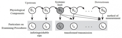
Railway track circuits consist of a series of trimming capacitors connected along the rails. The FDI tasks for this system are complicated by the fact that a malfunctioning upstream component (the trimming capacitor) influences the inspection signal of downstream components (located between the faulty capacitor and the receiver). This is depicted in a simplified form in Figure 1, where S1,...,SN represent the numbers of capacitors, and Ii, the inspection signal (measurement) for each capacitor. In the event of a fault in one of the capacitors, the inspection signals for all capacitors between the faulty one and the last one are affected. The fault isolation task must consider the geographical interconnectedness between subsystems, as an irregular measurement from one subsystem could signify a fault in that subsystem or any of the subsystems upstream of it.
A technique employing machine learning (neural networks, decision trees), and data fusion is demonstrated for detecting and isolating faults. The health status of individual capacitors is determined locally using a neural network or decision tree classifier, and this information is then aggregated to form a system-wide conclusion about the presence and location of a fault [11, 12].
Figure 1. A faulty subsystem (third capacitor) affects downstream subsystem inspection signals
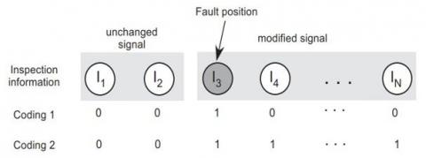
Determining an appropriate threshold for the dissimilarity between the network's outputs and the target outputs, which encapsulate the class membership of training patterns, is a critical phase during the training of a neural network classifier. Consequently, a method of output encoding must be finalized. This paper presents an analysis of two distinct strategies. The first strategy assigns a value of 1 to all output targets, with the exception of the one associated with the faulty system component (which is set to 0). This method could be referred to as "local coding". If the target outputs for both the downstream subsystems and the faulty subsystem are set to 0, the coding is described as distributed. Consequently, any classifier could be employed to determine whether a fault exists in a specific subsystem (local coding) or in the upstream subsystems (distributed coding).
Numerous approaches to classifier fusion have been proposed [13-15]. Empirical evidence suggests that the performance of classifiers can be enhanced through fusion for a variety of applications. Three categories of fusion approaches have been identified, based on the type of data provided by the individual classifiers:
– The first category encompasses approaches where each classifier only generates one class label output (crisp label); the most common choices here are majority vote and the behavior-knowledge space (BKS) technique.
– The second category, referred to as rank level decision type, involves each classifier creating a ranked list of labels. Fusion processes that yield these results are predicated on class set reduction, class set reordering, or a combination of both. The former strategy narrows down the pool of potential classes, while the latter aims to elevate the actual class to the top.
– The third and most extensive category of fusion methods aims to combine outcomes from classifiers that produce so-called soft labels in the range (0, 1). Belief function theories (also known as Dempster-Shafer or evidence theory) and Bayesian probability theory (or its extension, the Possibility theory) could provide a theoretical foundation for such actions.
The challenge of flexible recognition is frequently addressed using Nearest Neighbor Classifiers. Despite a limited number of reference symbols per class, this categorization principle offers substantial utility. The primary difficulty lies in incorporating a statistical understanding into the recognition task, which becomes particularly evident when multiple classifiers are deployed for the same task. To tackle this, a three-tiered process has been developed that converts the distance measurements of various classifiers into confidence values. Initially, each distance is transformed into the evidence function of a "specialist", who is accountable for a single reference pattern. Subsequently, the evidence function of an individual classifier is formed by amalgamating the votes of these specialists using Dempster/Shafer's theory of evidence. Finally, the outputs of all classifiers are integrated using the same theory. The efficacy of this method is assessed within the context of online script recognition, with the categorization outcomes compared against a previous method. The proposed approach generates an output vector for each distance classifier, making it suitable for statistically tailored classifiers across diverse pattern-matching contexts [16].
Railroad safety significantly depends on the effective inspection of freight vehicles' mechanical parts for potential malfunctions. However, traditional manual detection techniques have limited performance due to the minuscule size of the mechanical components. Additionally, conventional computer vision technology struggles with simultaneous detection of multiple classes of objects. Inspired by the proficiency of deep-learning-based one-step object detectors, this study introduces an innovative SSD-based detector, MFF-net. This detector leverages three modules to enhance detection accuracy and it collaborates with TFDS to facilitate efficient real-time fault detection in the small mechanical components of railway freight cars [17].
Over time, railway bridges exposed to harsh environments may experience a loss of effective cross-section at critical points, potentially leading to catastrophic failure. This paper proposes the application of Vibration-based Convolutional Neural Networks (CNNs) as a promising deep learning method for damage classification across varying extents and levels of cross section loss due to damages like corrosion [18].
As urban rail networks continue to expand in capacity and speed, concerns about their environmental impact intensify. This study delivers an artificial neural network (ANN)-based analysis of quantitative and qualitative predictors, which are gathered from field data collected during monitoring campaigns of ground vibration induced by light rail traffic in urban areas [19].
This research focuses on utilizing artificial neural networks to predict electric loads for railroad transportation. It investigates methods to predict the electrical demands of trains and other fixed rail infrastructure [20]. Key determinants of rail transportation energy consumption are analyzed, and a mathematical model for power usage, utilizing neural networks, is developed. An F-Fisher-based criterion is also proposed for evaluating neural network models. Moreover, the effective management of differential settlement along traffic lines is crucial. Hence, it's important to establish a rapid prediction model that can consider both vertical and parallel settlement profiles based on fundamental excavation information. A settlement profile along railways due to excavation is demonstrated using an empirical technique and a neural network. A database of 370 case records of field measurements of settlements was consulted to visualize the settlement profile features in three dimensions. The empirical technique employed a Rayleigh function distribution for settlement profiles perpendicular to the excavation, and a Gauss function distribution for vertical profiles. Observed data was also utilized to test and refine back-propagation neural networks. The results indicate that the model can accurately forecast the settlement along railways caused by an excavation [20].
In another study, accurate estimation of recoverable train delay can assist railway dispatchers in rescheduling trains and improving service reliability [21]. The researchers aimed to develop a model for predicting primary delay recovery (PDR) based on operational data from the Wuhan-Guangzhou (W-G) high-speed railway. Initial steps involved identifying significant delay factors such as dwell buffer time, running buffer time, extent of primary delay time, and impact of specific sections. An RFR model is proposed for predicting delay recovery in HSR trains experiencing primary delay. The RFR model outperforms conventional delay prediction models according to several performance analyses. Although the model's foundation was built using W-G HSR data, it could be easily extended to other HSR systems. The proposed approach could benefit professionals and academics interested in disruption management [21].
Finally, the challenge of detecting and categorizing railway switches is presented as a suitable application for Deep Neural Networks (DNN). The technique can be employed for landmark localization, environment perception, and condition monitoring of moving parts. A suitable DNN architecture, an anchor box ratio optimization strategy, and transfer learning compensate for the lack of large training datasets in the railway industry, as compared to the automotive sector. The study approach involves decomposing the problem of fault detection into smaller, capacitor-specific pattern recognition tasks, and the results are consolidated using the Dempster-Shafer theory.
Through better maintenance performance and use of maintenance possession time, this research aims to increase railway infrastructure capacity and service quality. The purpose of this research is to provide a framework for infrastructure managers to make data-informed maintenance choices at the tactical and operational levels of their organizations. The following is a detailed description of the study's goals:
4.1 The Dempster-Shafer Hypothesis
In this study have been created 4256 noise-filled signals at a variety of resistance values for a track circuit that had N=19 trimming capacitors so that we could assess how successful the strategy was. Six hundred and eight of the signals were flawless, while three thousand six hundred forty-eight of them had at least one defective capacitor that had a resistance between and r=1Ω and r=∞ (1). (The capacitor was removed) Estimates of performance were derived using the test set of 1075 signals after the dataset was first randomly segmented into three parts: training, validation, and test. For the purpose of determining whether or not our approach is effective, we compared it to a straightforward technique that makes use of a single multilayer perceptron to make a direct prediction about the location of the defective capacitor (position N+1 is used for fault-free scenarios). The advantages of our approach, which use an extra fusion step to identify and pinpoint a flaw in the system and the construction of as many classifiers as trimming capacitors, are thus quantified.
There was a comparison made between these approaches Here, we use the latter strategy, which offers a malleable framework for dealing with uncertainty and mediating conflicts among many classifiers, as the basis for our investigation. A new method has been revealed in this study to detect the circuit fault in railway systems by prediction of the error occurrence using Dempster-Shafer theory.
The automated train control system would not function without the track circuit. Its primary use is in determining the existence or train tracks in which no cars are allowed to go. The signaling system prevents collisions between trains by having them occupy separate sections of track. On French high-speed lines, the track circuit is an essential component of the track/vehicle transfer system. Coded information, such as the maximum allowed speed along a certain stretch of track due to safety considerations, is sent to the train through a designated carrier frequency.
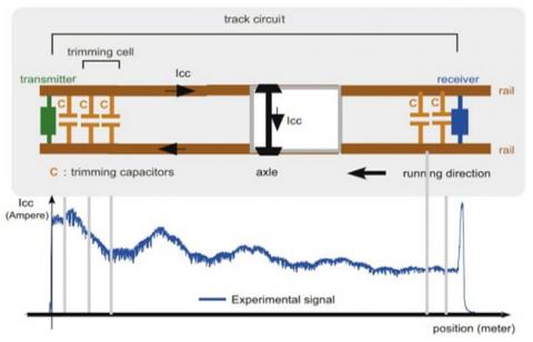
Several segments of track make up the rail line. Shown in Figure 2 is the track circuit for each of them, which consists of:
– a transmitter at one of the terminals sends out alternating current that varies in frequency;
– the potential transmission line formed by the two railroads;
– there is a receiver at the opposite end of the segment of track that consists mostly of a trap circuit and is used to prevent data from being sent to the next segment of track;
– correction for the track's inductive behavior is accomplished by fine-tuning capacitors linked between the rails at a fixed distance apart. The transmission level may then be increased by performing electrical tuning to reduce the loss of transmitted current. In order to calculate the total number of compensation points, we need to know the length of the track section and the carrier frequency.
Figure 2. An illustration of an inspection signal and a circuit diagram for a track
The train's wheels and axles create a short circuit with the rails, which are part of the track circuit, allowing for detection of the track. When a train is present in a specific stretch, the signal along the track circuit breaks down because the train's wheels act as a short. To indicate that the area is occupied, the received signal must drop below a certain level. In order to make the transmitted information section-specific and to mitigate the effects of longitudinal interference and transverse crosstalk, four frequencies are used for adjacent and parallel track circuits. Both the sender and the receiver may keep electrical signals separate from those of other circuits on the track by using tuned circuits (capacitance and inductance).
In order to maintain the system's required safety and availability standards, it is crucial that any failures in the track circuit's multiple components (due to, for example, age, environment, or track maintenance operations) be identified as soon as possible. Problems with signaling triggered by the severe attenuation of the sent signal that might result from such failures. Maintainers may be alerted to potential transmission quality issues such track circuit breakdowns via system diagnostics.
An inspection truck fitted with a sensor in front of the front axle used to create a defect diagnostic system based on the vehicle's own data. At each place along the track, the inspection train acts as a "shunt," interrupting the circuit, and allowing the sensor coils to record the short-circuit current (Icc) carrier current level (Figure 2).
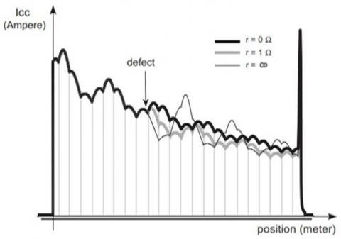
Capacitor internal resistance impacted by flaws, which will be the topic of this study. To account for the deviation from the ideal behavior of the capacitor, most of which is due to dielectric aging, we include a serial resistance r that is zero (or weak) while the capacitor is healthy and develops when it is malfunctioning. The system can be realistically simulated, flaws and all, thanks to the development of an electrical model. The lack of fault and the presence of a faulty 10th capacitor are represented by the Icc signals shown in Figure 3. By analyzing the measurement signal, the fault detection and isolation system may ascertain the functioning status of the track circuit.
The two findings shown in Figure 3 form the basis of the suggested technique:
– the Examining: The characteristic shape of an Icc signal is a series of arcs, or catenary curves;
– in the case of a problem, only the segment of the signal that is further from the transmitter will be impacted, while the segment closer to the fault will be untouched.
Figure 3. An example of a simulated Icc signal with and without a faulty 10th capacitor
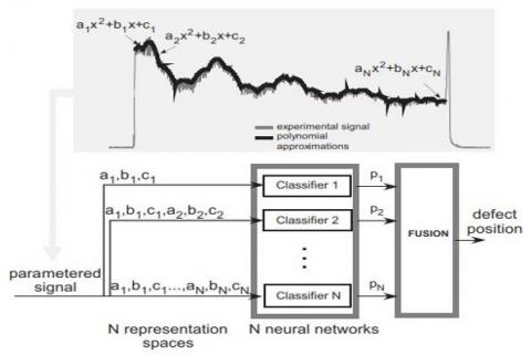
Similar to a trim cap: a quadratic polynomial used to approximatively describe an arch.
The suggested technique involves parsing the Icc signal for relevant characteristics and then developing a separate classifier for each trimmer. The results of these individual elementary classifiers are then integrated using the language of belief functions as a representation. After much deliberation, a conclusion is reached as to whether or not a defect exists and where it found.
The core ideas of the Dempster-Shafer theory of belief functions (also known as the Evidence theory) will be elucidated. Shafer is the one who came up with the idea and built this uncertain reasoning framework. The Bayesian probability theory considered as having been extended by this. The transferable belief model is a specific interpretation of the Dempster–Shafer theory that has been offered (TBM). The TBM is built on, point of credibility when ideas are considered plausible and swinish echelon at which choices made.
Only the terms needed for the diagnostic approach described below will be defined here.
The collection of feasible solutions to an issue is the discerning framework; designate it with the symbol; ($\Theta$) - Here, it is assumed that has a finite value:
$\Theta=\left\{\theta_1, \theta_2, \ldots \theta_n\right\}$ (1)
When we assumed that we have a basic belief assignment (BBA), we mean that we have a function m from;(2$\Theta$) to [0,1]- that allocates a "mass of belief" to each subset A of the discerning frame;($\Theta$), such that
$\sum_{A \subseteq \Theta} m(A)=1$ (2)
Because it is hard to settle on a specific subset of A, we may use the; (m(A)), represent the basic belief mass to quantify the weight we give to the evidence that supports attributing the belief that we have to set; (A⊆ $\Theta$), represent the quantify the weight. A focused set is any two-element set; (A⊆ $\Theta$), such that; (m(A)≻0), It is claimed that a BBA is normal if and only if; m(ϕ)=0, where; (ϕ), - is the empty set. The amount; (m(ϕ)) might be understood to represent the share of faith that is staked on the possibility that none of the hypotheses in are correct (open-world assumption). In the case of; (m($\Theta$)), m is considered a vacuous BBA since it shows a complete lack of understanding of the issue at hand.
Let's say that we're studying a system whose states are denoted by; ($\Theta$={θ1,θ2,θ3}), with (θ1),representing the normal state. Let's assume we have evidence that suggests the system is in a deficient state with a confidence level of (0.9), These findings are summed up by the following BBA:
$\begin{gathered}m_1\left(\left\{\theta_2, \theta_3\right\}\right)=0.9 \\ m_1(\Theta)=0.3\end{gathered}$
As the data simply suggests that the system is in a defective condition without directing attention to either; (θ2 or θ3)- we make note that the mass; (0.9) is associated with; (θ2, θ3)- Due to a lack of supporting data, we do not attribute the remaining (0.3) of mass to (θ1), It clings to the whole framework of perception while remaining uncommitted.
To combine several BBAs stated on the same frame of understanding, Smets developed the conjunctive rule of combination, commonly known as the unnormalized Dempster's rule. In order to apply this rule, the several BBAs must be grounded on distinct pieces of evidence. Consider two BBAs ((m1)) and ((m2))- This conjunctive conjunction, represented by; (m1∩m2)-yields a BBA, which is defined for all (A⊆ m2); as
$m_1 \cap m_2(A) \sum_{B C \Theta: B \cap C=A}\quad m_1(B) m_2(C)$ (3)
Associative and commutative, this rule is quite useful. As a result, we have two options for directly merging n BBAs m1, …, mn: (a) using (3) iteratively, or (b) using the method below.
$m_1 \cap \ldots m_n(A)=\sum_{B_1 \cap \ldots \cap B_n=A}\quad m_1\left(B_1\right), \ldots, m_n\left(B_n\right)$ (4)
The value of ($m(\phi)$), which is applied to the empty set, seen as a quantitative representation of the tension between the two inputs.
Case 2 Let's say that more information indicates the system is not in state (θ2), with a confidence level of (0.7), continuing the scenario established in Case 1. The following BBA might be used to portray this evidence:
$\begin{gathered}m_2\left(\left\{\theta_1, \theta_3\right\}\right)=0.7 \\ m_2(\Theta)=0.4\end{gathered}$
The BBA (m=m1∩m2), is defined as the sum of (m1) and (m2) which is obtained by using (3).
$\begin{gathered}\left(\left\{\theta_3\right\}\right)=0.8 \times 0.6=0.48 \\ m\left(\left\{\theta_2, \theta_3\right\}\right)=0.8 \times 0.4=0.32 \\ m\left(\left\{\theta_1, \theta_3\right\}\right)=0.2 \times 0.6=0.12 \\ m(\Theta)=0.2 \times 0.4=0.08\end{gathered}$
The multitudes are still adding up to one, as we can see.
One way to account for the credibility of a source is to apply a discount rate; (1-α) -on the original BBA m, where; (α)-is a coefficient between zero and one. The discount rate increases as the level of trustworthiness decreases. With this BBA in hand αm
$\begin{gathered}{ }^\alpha m(A)=\alpha(A) \forall A \subset \Theta \\ { }^\alpha m(\Theta)=1-\alpha[1-m(\Theta)]\end{gathered}$ (5)
By shifting some of the weight of belief from; (α) to ($\Theta$)- the information content of the BBA suffers. The trustworthiness of the source is represented by the coefficient; (α), When (α=1) holds, the belief function remains unaltered, and we have complete faith in the credibility of the source. As approaches 0, the resultant BBA is more like the empty belief function; (m($\Theta$)=1), -which means that the source's information is ignored. There are a number of approaches that have been presented to use data to get the best possible answer for α.
Case 3 the following scenario: we are going to flip a coin, and our expectation of the result is shown on the frame; ($\Theta$={Head, Tails})- If the coin is honest, we may express our faith in; ($\Theta$)-using the BBA below.
$\begin{aligned} & m(\{\text { Head }\})=0.5 \\ & m(\{\text { Tails }\})=0.5\end{aligned}$
A Bayesian BBA is a kind of BBA in which the focus sets are all unique. This type of BBA is comparable to a probability distribution. Let's pretend for a moment that we have just a; (0.8) -level of confidence in the fairness of the coin. In such case, a discount off the aforementioned BBA is in order; (1-α=1-0.8=0.4) -The BBA after discounting is
$\begin{gathered}{ }^\alpha m(\{\text { Head }\}) 0.8 \times 0.5=0.4 \\ { }^\alpha m(\{\text { Tails }\}) 0.8 \times 0.5=0.4 \\ { }^\alpha m(\Theta)=0.4\end{gathered}$
Some of the weight seems to have been moved to the discernment framework, which a result of a misunderstanding of the odds.
The credal level is where one's beliefs are entertained, whereas the pianistic level is where one's BBAs are converted into probability distributions and used to form decisions in line with the idea of maximal expected benefit.
When a decision has to be made, the BBAs are transformed into probabilities. The BBA m is transformed using the pianistic procedure defined above, and the resulting pianistic probability function, BetP is then constructed.
$\operatorname{BetP}(\theta)=\sum_{\{B \subseteq \Theta, \theta \in B\}} \frac{1 m(B)}\quad{|B| 1-m(\phi)}\quad \forall \theta \in \Theta$ (6)
where, the cardinality of (B) - is denoted by |B|, - it is taken for granted that (m(ϕ)≺1)
For all practical purposes, this definition assumes that; (m(B)) -is uniformly distributed among; (B) - constituent parts in the absence of any other information (B⊆$\Theta$) - For decision making in accordance with traditional Bayesian decision; theory, the pianistic probability is a useful classical measure of probability.
$\begin{gathered}{BetP}\left(\left\{\theta_1\right\}\right)=\frac{0.12}{2}+\frac{0.09}{3} \simeq 0.08 \\ Bet P\left(\left\{\theta_2\right\}\right)=\frac{0.33}{2}+\frac{0.09}{3} \simeq 0.2 \\ BetP\left(\left\{\theta_3\right\}\right)=0.49+\frac{0.33}{2}+\frac{0.13}{2}+\frac{0.09}{3} \simeq 0.75\end{gathered}$
Case 4 recalling the BBA m from equation above, represented the pianistic probability function.
4.2 Methods for diagnosis
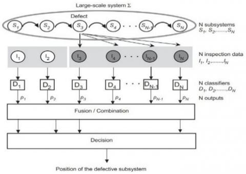
A high-level schematic of the proposed diagnostic system's whole architecture is shown in Figure 4. The track circuit is shown as the system Σ, and the N subsystems; (S1, …, SN) -are the trimmers. The application's stated goal is to identify the location of the faulty capacitor should a problem be found in any of these capacitors. One faulty capacitor is thought to be the maximum. The measured information for capacitor; Si, -is shown as Ii, in Figure 4. The vector of information; (I1, …, IN) - consists of the points along the curve in Figure 2. As demonstrated by the arrows connecting; S3 and (I3, …, IN), a failure in capacitor; (S3)- would alter the measurement data (i. e., the shape of catenary curves) pertaining to all capacitors downstream.
A diagram of the proposed system's ; (N)- local classifiers is shown in Figure 4; ((D1, …, DN) -), - A priori, each local classifier ;(Di)- tasked with learning to make a prediction about the health of either capacitor; (Si) or the health of the capacitors upstream from it. The terms "local coding" and "distributed coding" will be used to describe these two methods from now on. Although both of these strategies make sense on the surface, we'll go into them more below.
Figure 4. An overview of the fault isolation and localization methodologies guiding principles
To do this, feature values are taken from inspection data and fed into a classifier (Di), which then calculates a probability based on the data; (Pi). After that, the preferred encoding modifies the output into a Dempster-Shafer mass function mi. In order to apply pignistic probability to identify whether or not a defect exists and, if so, where it is located, we must first combine the N mass functions into a single mass function m using Eqns. (3), (4), (6).
4.3 Determining important characteristics
Figure 3 depicts an Icc curve, which is the shape the inspection data take, The space for measurements is thus defined. Segments of the Icc curve have an arched shape. These arcs stand in for individual capacitors that serve as fine-tuners. In order to construct a sparse representation of the data, each segment was approximated by a quadratic polynomial, and its three coefficients; (ai, bi and ci) - were used as features in the process (Figure 5). Hence, a total of (3N)- characteristics were used to characterize the whole Icc curve.
Together with the i th capacitor for fine-tuning. Hence, classifiers' feature spaces are nesting.
In this study, we focus on probabilistic classifiers such as those based on neural networks or decision trees. As was mentioned before, every local classifier Di has the potential to be educated to recognize defects in either capacitor Si or any other capacitor that lies between S1 and Si As can be shown in Figure 6, the encoding of neural network outputs is affected because of the nature of the learning job that neural networks are assigned when they are used as classifiers. Let's pretend that capacitor Si (at i=3 in Figure 6) has developed a defect. We shall examine two scenarios:
Figure 5. Taking out features
– in order to put into practice, the local coding that is shown in Figure 6, we would begin by setting the intended output for classifier Di, to the value 1, while leaving the desired outputs for the other classifiers at the value 0.
– with dispersed coding (Figure 6 coding 2), classifiers Dj with j ≥ i have 1 set as their intended output and 0 set as the outcome of every other classifier.
As a matter of first principles, distributed coding seems to be the best option for taking into consideration the physical proximity of individual systems. Yet, this research will investigate and test both approaches.
Due to the fact that classifiers Di= (i=1, ..., N) only analyze regional data, their results must be averaged before a definitive conclusion can be drawn about whether or not a faulty capacitor is present and where it found. Classifier results are represented in Dempster-Shafer form, and then merged using Dempster's rule (3), (4).
A Dempster-Shafer model cannot be constructed without first defining the context in which judgments are made, in this particular instance, we will utilize set $\Theta$= {1, ..., N, N+1}, where N refers to the total number of capacitors included inside the rail circuit. Each unique pair {i}, i =1, ..., N+1 represents a distinct potential fault location. The lack of a problem corresponds to the virtual position N+1 In this section, we will begin by discussing the issue of local coding, and then we will go on to discuss the scenario of distributed coding, detailing how the outputs of classifiers are translated into mass functions and integrated.
4.4 Combining several classifiers using neighborhood codes
Using local encoding, if classifier Di, returns a 1, then the failure is assumed to be in capacitor Si Figure 6. And if there isn't, then something's wrong.
Figure 6. The N classifiers are trained using one of two output coding techniques
If capacitor S3 is faulty, the N classifiers are trained using one of two output coding techniques. Just the intended result of classifier D3 is coded as a 1 using local coding (code 1).
All classifiers Dj with j ≥ 3 have their targets set to 1 using dispersed coding (coding 2) in a capacitor of value Sj whereby either j ≠ i or {i} holds true. It follows that BBA mi, with the singleton {i} and its complement {i}/ Θ as its focal sets, used to represent Di,'s classification results.
$m_i(\{i\})=P_i, \quad m_i(\Theta /\{i\})=1-P_i$ (9)
Characterized by the fact that the output of classifier Di, is denoted by Pi $\in$[0,1].
When applying the unnormalized version of Dempster's rule (4) to the combination of the N BBAs m1, …mN the result is a BBA m that has N+1 focal sets. These sets are referred to as singletons and the empty set respectively. The following is a transcription of the phrase that may be found on this BBA:
$\begin{gathered}m(\{i\})=P_i \prod_{J \neq i}\left(i-P_j\right) \forall i=1, \ldots, N \\ m(\{N+1\})=\prod_{i=1}^N\left(1-P_i\right)\end{gathered}$
$m(\phi)=1-\sum_{i=1}^{N+1} m(\{i\})$ (10)
Let us suppose for the moment that we are going to reduce the output of each classifier by a rate of 1-αi with 0≤ α ≤1. As will be shown in Section 5, the discount rate figured by using the classifier error as a determining factor. After this, the value of BBA mi, which represents the output of classifier Di, is
$m_i(\{i\})=\alpha_i P_i, \quad m_i(\Theta /\{i\})=\alpha_i\left(1-P_i\right), \quad m_i(\Theta)=1-\alpha_i$ (11)
An unnormalized variant of Dempster's rule is used to combine these N BBAs into a BBA m, which described as follows.
$\begin{gathered}m(\{i\})=\alpha_i P_i \prod_{j \neq i}\left[\alpha_j\left(1-P_j\right)+\left(1-\alpha_j\right)\right] \forall i=1, \ldots, N, \\ m(\{N+1\})=\prod_{i=1}^N \alpha_i\left(1-P_i\right)\end{gathered}$
$m(A)=\prod_{i \notin A} \alpha_i\left(1-P_i\right) \prod_{i \in A}\left(1-\alpha_i\right) \forall A \subset \Theta, N+\in A, 1 \prec N$ (12)
The remaining portion of the mass being allotted to the set that is empty. If the coefficient indexes are negative or 0, as is often believed to be the case, then the products in the preceding phrases disappear.
Let's assume that the classifier Di 's output is 0, and that distributed coding was employed. Thus, either there is an issue between Si+1 and SN or there isn't a problem there. On the other hand, if classifier Di 's output is 1, then it is clear that there is an issue with the link between S1 and Si. Hence, the following BBA used to describe the data provided by the classifier Di.
$m_i([1, i])=P_i, m_i([i+1, N+1])=1-P_i$ (13)
where, [1, i] represents the range of numbers from 1 to i and Pi $\in$[0,1] represents the output of the classifier Di, as in the previous illustration.
When Dempster's rule (4) is applied to the combination of m1, …mN the following BBA is produced:
$\begin{gathered}m(\{i\})=\prod_{j=1}^{i-1}\left(1-P_j\right) \prod_{k=i}^N P_K \forall i=1, \ldots, N, \\ m(\{N+1\})=\prod_{i=1}^N\left(1-P_i\right),\end{gathered}$
$m(\phi)=1-\sum_{i=1}^{N+1} m(\{i\})$ (14)
The BBA produced by the ith classifier, mi, changes to reflect the discount rate of 1-αi applied to all BBAs reflecting classifier Di's output, as previously.
$m_i([1, i])=\alpha_i P_i, \quad m_i([i+1, N+1])=\alpha_i\left(1-P_i\right)$
$m_i(\Theta)=1-\alpha_i$ (15)
Dempster's rule, in its unnormalized version, was applied to this set of BBAs, and the outcome is what we have right now.
$\begin{gathered}m(\{1\})=\alpha_1 P_1 \prod_{j=2}^N\left[\alpha_j P_j+\left(1+\alpha_j\right)\right], \\ m=(\{2\})=\alpha_2 P_2 \alpha_1\left(1-P_1\right) \prod_{j=3}^N\left[\alpha_j P_j+\left(1-\alpha_j\right)\right], \\ m(\{i\})=\alpha_i P_i \alpha_{i-1}\left(1-P_{i-1}\right) \prod_{j=i+1}^N\left[\alpha_j P_i+\left(1-\alpha_j\right)\right] \prod_{K=1}^{i=2}\left[\alpha_K\left(1-P_K\right)+\left(1-\alpha_K\right)\right] \forall i \in[3 i N], \\ m(\{N+1\}) \alpha_N\left(1-P_N\right) \prod_{j=1}^{N-1}\left[\alpha_j\left(1-P_j\right)+\left(1-\alpha_j\right)\right], \\ m([i, j])=\alpha_{i-1}\left(1-P_{i-1}\right) \alpha_j P_j \prod_{m=i}^{j-1}\left(1-\alpha_m\right) \prod_{K=j+1}^N\left[\left(1-\alpha_j\right)+\alpha_K P_K\right] \prod_{l=1}^{i-2}\left[\alpha_1\left(1-P_l\right)+\left(1-\alpha_i\right)\right] \forall i \prec j[[i, j] \subset \Theta, \end{gathered}$
$m(\Theta)=\prod_{i-1}^N\left(1-\alpha_i\right)$ (16)
Empty set receives the remaining fraction of the mass allocation.
For example, let us take into consideration a made-up system that is comprised by N=3 different subsystems. The discerning framework is denoted by the equation Example. Let us take into consideration a made-up system that is comprised by N=3 different subsystems. The discerning framework is denoted by the equation $\Theta$={1, 2, 3, 4}.
Classifier $\mathrm{D}_1: m_1(\{2,3,4\})=1-p_1$,
$m_1(\{1\})=p_1 \text {, }$
Classifier $\mathrm{D}_2: m_2(\{3,4\})=1-p_2$,
$m_2(\{1,2\})=p_2,$
Classifier $\mathrm{D}_3: m_3(\{4\})=1-p_3$,
$m_3(\{1,2,3\})=p_3 \text {, }$
Hence, the total BBA is
$\begin{gathered}m(\{1\})=p_1, p_2 p_3, \\ m(\{2\})=\left(1-p_1\right) p_2 p_3, \\ m(\{3\})=\left(1-p_1\right)\left(1-p_2\right) p_3, \\ m(\{4\})=\left(1-p_1\right)\left(1-p_2\right)\left(1-p_3\right), \\ m(\phi)=1-\sum_{i=1}^4 m(\{i\})\end{gathered}$
Without taking into account discounts, the above are the various BBAs that are supplied by the classifiers.
5.1 Present railway maintenance procedures
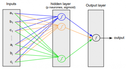
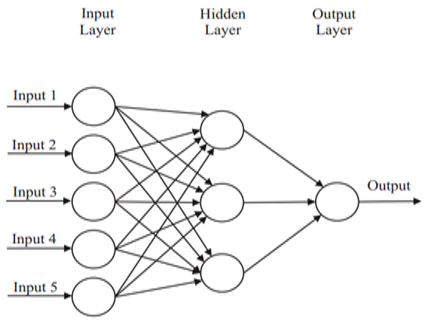
Using a sigmoid hidden layer composed of seven neurons and a linear output layer consisting of a single neuron, we perform multilayer perceptron regression. The location of the fault was input, and the 20×3=60 parameters; (ai, bi, ci) of the Icc curve, where; I =1, ...,20- were produced. When there were no problems with the system, it would switch to using the; N+1- virtual location. It is the standard procedure that everyone follows. This network was trained to attain a minimal mean square error (MSE) between its fault location estimations and the actual fault sites for the whole of the training set. This was accomplished via the use of a minimum mean square error target. The number of hidden neurons ranged from three to fifteen in this experiment, with seven yielding the best results on the validation set. Figure 7 shows the process of applied sigmoid function and Table 1 illustrated number of hidden nodes for each neural network classifier. It is practical to employ simulation techniques to evaluate its applicability in high-velocity traffic circumstances. In high-speed traffic situations, the model may be used to ascertain the potential capacity of a single-track element (block, artificial structure) (Figure 8).
Figure 7. Applying sigmoid function
Figure 8. Capacity as a function of single-track segment length, graphically shown
Table 1. Number of hidden nodes
|
i |
1 |
2 |
3 |
4 |
5…17 |
|
Numbers of hidden layers |
2 |
3 |
4 |
6 |
7 |
5.2 Capacity-boosting maintenance
Using the two encoding procedures (with and without discounting) described we fuse local classifiers from neural networks (feed forward) and decision trees. With these additions, we now have eight distinct fusion-based approaches. The classifiers in the neural networks have only one tan-sigmoid hidden layer and one sigmoid output neuron (Figure 7). Table 1 displays the total number of hidden nodes for each classifier, which was determined by lowering the error criterion for the validation set. Each neural network was trained a total of 100 times using randomized initial circumstances. The CART technique was the algorithm used to create the tree of decisions.
Classifier; Di- discount rate, 1- αi was calculated using its mean squared error in cases when discounting was employed (MSEi) generated from the test data as:
$1-\alpha_i=\frac{0.5 M S E_i}{\max _j\left(M S E_j\right)} i=1, \ldots, N$ (17)
As a perfect classifier with MSEi=0 would incur no discount at all, we discounted the worst classifier at a rate of 0.5.
The findings from the different analysis are shown in Table 2 have been computed the rates of correct detection (CD), false alarms (FA), non-detections (ND), and correct rejections (CR) using the whole data set, which included both defective and healthy signals (CR). Figure 9 shows the classifier based on neural network.
Figure 9. Design of a classifier based on an iteration of a neural network
Table 2. Results analysis
|
Type of error |
No fault |
Fault position k |
|
No fault |
CR |
ND |
|
NCR |
NDN |
|
|
Decision fault position k |
FA |
CD |
|
NFA |
NCD |
|
|
Fault position $j \neq K$ |
– |
FL |
|
– |
NFL |
Distinguished between correct localizations (CL=CD+CR); and false localizations; (FL=CD+CR)- to take into consideration situations in which a failure is correctly diagnosed but incorrectly localized inside the system; (FL).
The following notation used to determine a number of performance measures, where; N 0- is the number of good signals; N 1-is the number of bad signals, and; N X- is the number of cases in category; X- (where; X- - is (CD, CR, FL) or ((FA):
$t_{C D}=\frac{N_{C D}+N_{C R}+N_{F L}}{N_0+N_1}, \quad t_{C L}=\frac{N_{C D}+N_{C R}}{N_{C D}+N_{C R}+N_{F L}}$
$t_{F A}=\frac{N_{F A}}{N_0}, \quad t_{N D}=\frac{N_{N D}}{N_1}$
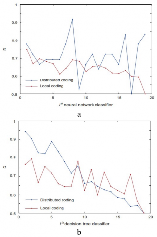
There is also an examination of the differences and similarities between the outcomes acquired via the use of neural networks and decision tree classifiers (DT); the discount rates we calculated using (18) to combine the classifier results. Except for neural network classifiers that make use of distributed coding; αi- coefficients have a tendency to decrease with; i -which indicates that classifiers are heavily discounted as i rises. In addition, the learning process gets more sophisticated the closer we get to the receiver.
Fusion approaches fared better than the reference regression approach across all possible encoding schemes, while neural networks beat decision trees. The proper localization rate also climbed to well over 94%, and the rate at which it correctly detects objects was similarly boosted. As an added bonus, compared to the regression technique (~60%), the fusion methods only caused a marginal increase in false positives (~1%). In fact, the goal of the regression technique is to find the problem and zero in on its source at the same time. Estimates for the fault's location varied between 1 to N+1; where N+1, - is the fault-free system s virtual location and; N - is the total number of subsystems to be more precise, if the predicted location is; N+1 - (in a fault-free system) rather than (in a faulty one, with the fault located at position; N - a false alarm will be generated. For this reason, this technique has a high incidence of false positives. It is clear, however, that even the best detection algorithms result in some missed cases.
The incidence of non-detection was greater when using local coding rather than spread coding. This is because the training database has an uneven number of cases from each class. Each classifier picked up more 0s (no fault) than 1s (error) while applying local coding.
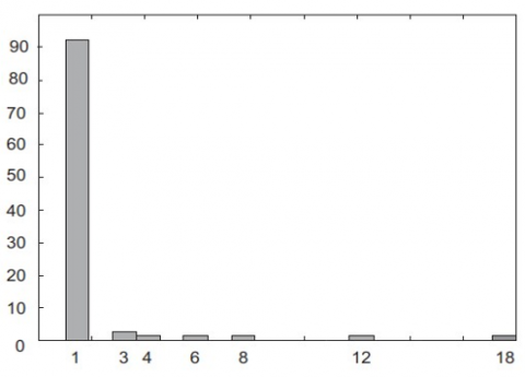
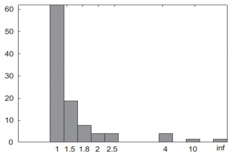
Some gains were made once discounting was included, with higher rates of accurate detection and lower rates of false alarms offsetting a fall in the rates at which proper localizations were achieved. Reason for this is the low mean square error achieved by all the local classifiers. For both decision trees and neural networks Figure 8, local coding provides more precise localization results than distributed coding. The quantity of localization errors analysed by looking at the histogram of errors between the actual position and estimated of the fault, as illustrated in Figure 10, for fusion with distributed coding and no discounting. The localization error was 1 in 92.2% of the tests in Figure 11, which is acceptable for this application. To add, when a problem was not precisely located, we approximated the histogram of the damaged capacitor's serial resistance (Figure 12). In the vast majority of cases (80.3%), the resistance of the faulty capacitor was lower than 1.4 ohm.
As a result, it is reasonable to infer that the suggested method successfully identified the vast majority of errors. Even with dispersed code, localization was successful, since most defects were caused by tiny flaws that could be pinpointed to the nearest neighbour of the faulty subsystem. The best outcomes were achieved by using a neural network technique that included both distributed coding and discounting.
Figure 10. The coefficients of discounting for each classifiers results: a ‒ is neural network; b ‒ is a decision trees classifier
Figure 11. Variation in fault location estimates as a function of distance from the actual fault location (NN, distributed coding)
Figure 12. In the event of mis localization (NN, dispersed coding), a histogram of the serial resistance is shown below
Experts in railway management and a specialist in railway maintenance reviewed the comparative findings. The potential reductions in both the work for maintenance staff and the obstruction for train operators have been welcomed by everybody. The new model produces a favorable timetable, although one that requires more nights overall. Five nights a week, on average, are set aside for scheduled maintenance activities, however this affects only a fraction of the network. This suggests that there is still opportunity for new endeavors in other areas. Since the hindrance points cannot be simply translated into these numbers, a thorough examination of the schedule is required to determine the exact number of trains hampered. When the electricity of the overhead wire is turned off for repair, the number of trains that are impeded is calculated based on the number of trains required to start the schedule on a typical workday.
Data-driven maintenance planning and scheduling is essential for efficient track possession management and maximizing availability. If put into practice, the study's method of analysis and modeling for planning and optimizing track geometry maintenance would help cut down on track possession time. The study found that there is room to increase the efficiency of possession time use by optimizing tamping cycle length and shift duration and enhancing the tamping process. Intervention choices, consolidation of spot failure corrective procedures, and reduction of total time on track for geometry maintenance over a certain planning horizon were all aided by the degradation model and the defined schedule optimization issue. Following are some final thoughts on the case study:
[1] De Bruin, T., Verbert, K., Babuška, R. (2016). Railway track circuit fault diagnosis using recurrent neural networks. IEEE Transactions on Neural Networks and Learning Systems, 28(3): 523-533. https://doi.org/10.1109/TNNLS.2016.2551940
[2] Chen, J., Roberts, C., Weston, P. (2008). Fault detection and diagnosis for railway track circuits using neuro-fuzzy systems. Control Engineering Practice, 16(5): 585-596. https://doi.org/10.1016/j.conengprac.2007.06.007
[3] Wang, M., Zheng, H., Huang, Z. (2016). Fault prognosis of track circuit based on GWA fuzzy neural network. In Proceedings of the 2015 International Conference on Electrical and Information Technologies for Rail Transportation: Electrical Traction, pp. 473-481. https://doi.org/10.1007/978-3-662-49367-0_48
[4] Hu, L.Q., He, C.F., Cai, Z.Q., Wen, L., Ren, T. (2019). Track circuit fault prediction method based on grey theory and expert system. Journal of Visual Communication and Image Representation, 58: 37-45. https://doi.org/10.1016/j.jvcir.2018.10.024
[5] Alvarenga, T.A., Cerqueira, A.S., Filho, L.M., Nobrega, R.A., Honorio, L.M., Veloso, H. (2020). Identification and localization of track circuit false occupancy failures based on frequency domain reflectometry. Sensors, 20(24): 7259. https://doi.org/10.3390/s20247259
[6] Chen, J., Roberts, C., Weston, P. (2007). Neuro-fuzzy fault detection and diagnosis for railway track circuits. IFAC Proceedings Volumes, 39(13): 1366-1371. https://doi.org/10.1016/b978-008044485-7/50230-x
[7] Havryliuk, V. (2020). ANFIS based detecting of signal disturbances in audio frequency track circuits. In 2020 IEEE 2nd International Conference on System Analysis & Intelligent Computing (SAIC), Kyiv, Ukraine, pp. 1-6. https://doi.org/10.1109/saic51296.2020.9239127
[8] Peterson, C., Söderberg, B. (1989). A new method for mapping optimization problems onto neural networks. International Journal of Neural Systems, 1(1): 3-22. https://doi.org/10.1142/s0129065789000414
[9] Kadhim, I.B., Khaleel, M.F., Mahmood, Z.S., Coran, A. N.N. (2022). Reinforcement learning for speech recognition using recurrent neural networks. In 2022 2nd Asian Conference on Innovation in Technology (ASIANCON), Ravet, India, pp. 1-5. https://doi.org/10.1109/asiancon55314.2022.9908930
[10] Kamal, A.E., Mahmood, Z.S., Nasret, A.N. (2022). A new methods of mobile object measurement by using radio frequency identification. Periodicals of Engineering and Natural Sciences, 10(1): 295-308. https://doi.org/10.21533/pen.v10i1.2615
[11] Mahmood, Z.S., Nasret, A.N., Mahmood, O.T. (2021). Separately excited DC motor speed using ANN neural network. In AIP Conference Proceedings, 2404(1): 080012. https://doi.org/10.1063/5.0068893
[12] Denoeux, T. (2000). A neural network classifier based on Dempster-Shafer theory. IEEE Transactions on Systems, Man, and Cybernetics-Part A: Systems and Humans, 30(2): 131-150. https://doi.org/10.1109/3468.833094
[13] Beynon, M., Cosker, D., Marshall, D. (2001). An expert system for multi-criteria decision making using Dempster Shafer theory. Expert Systems with Applications, 20(4): 357-367. https://doi.org/10.1016/s0957-4174(01)00020-3
[14] Mandler, E., Schümann, J. (1988). Combining the classification results of independent classifiers based on the Dempster/Shafer theory of evidence. In Machine Intelligence and Pattern Recognition, 7: 381-393. https://doi.org/10.1016/b978-0-444-87137-4.50032-1
[15] Yang, C., Li, Z., Guo, X., Yu, W., Jin, J., Zhu, L. (2019). Application of BP neural network model in risk evaluation of railway construction. Complexity, 2019: 2946158. https://doi.org/10.1155/2019/2946158
[16] Ye, T., Zhang, Z., Zhang, X., Chen, Y., Zhou, F. (2021). Fault detection of railway freight cars mechanical components based on multi-feature fusion convolutional neural network. International Journal of Machine Learning and Cybernetics, 12: 1789-1801. https://doi.org/10.1007/s13042-021-01274-z
[17] Ghiasi, A., Moghaddam, M.K., Ng, C.T., Sheikh, A.H., Shi, J.Q. (2022). Damage classification of in-service steel railway bridges using a novel vibration-based convolutional neural network. Engineering Structures, 264: 114474. https://doi.org/10.1016/j.engstruct.2022.114474
[18] Komyakov, A.A., Erbes, V.V., Ivanchenko, V.I. (2015). Application of artificial neural networks for electric load forecasting on railway transport. In 2015 IEEE 15th International Conference on Environment and Electrical Engineering (EEEIC), Rome, Italy, pp. 43-46. https://doi.org/10.1109/eeeic.2015.7165296
[19] Tang, Y., Xiao, S., Zhan, Y. (2019). Predicting settlement along railway due to excavation using empirical method and neural networks. Soils and Foundations, 59(4): 1037-1051. https://doi.org/10.1016/j.sandf.2019.05.007
[20] Jiang, C., Huang, P., Lessan, J., Fu, L., Wen, C. (2019). Forecasting primary delay recovery of high-speed railway using multiple linear regression, supporting vector machine, artificial neural network, and random forest regression. Canadian Journal of Civil Engineering, 46(5): 353-363. https://doi.org/10.1139/cjce-2017-0642
[21] Jahan, K., Niemeijer, J., Kornfeld, N., Roth, M. (2021). Deep neural networks for railway switch detection and classification using onboard camera images. In 2021 IEEE Symposium Series on Computational Intelligence (SSCI), Orlando, FL, USA, pp. 1-7. https://doi.org/10.1109/ssci50451.2021.9659983