Juan Geng* | Liang Yan | Yichao Liu
© 2020 IIETA. This article is published by IIETA and is licensed under the CC BY 4.0 license (http://creativecommons.org/licenses/by/4.0/).
OPEN ACCESS
In recent years, tensor completion problem, as a higher order generalization of matrix completion, has received much attention from scholars engaged in computer vision, data mining, and neuroscience. The problem is often solved by convex relaxation, which minimizes the tensor nuclear norm instead of the n-rank of the tensor. However, tensor nuclear minimizes all the singular value at the same level, which is unfair to large singular values. To solve the problem, this paper defines a log function of tensor, and uses it as an approximation of tensor rank function. Then, a simple yet efficient log-based algorithm for tensor completion (Log-TC) was proposed to recover an underlying low n-rank tensor. The Log-TC was verified through experiments on randomly generated tensors and color image inpainting, in comparison with two tensor completion algorithms: fixed point iterative method for low-rank tensor completion (FP-LRTC) and fast low rank tensor completion algorithm (FaLRTC). The results show that our algorithm greatly outperformed the two contrastive methods.
tensor completion, log function of tensor, image inpainting, tensor decomposition
In the era of data explosion, tensors gain more and more attention thanks to their excellence in information preservation and structural properties. Tensors can be viewed as natural higher-order generalization of vectors and matrices. Therefore, many questions of tensors can be generalized from vectors and matrices.
Tensor completion, a natural generalization of matrix completion, has long been a research hotspot. As an imputation method for missing data, tensor completion aims to estimate missing data from very limited information of observed data. To date, this problem has been widely applied in recommendation system [1-7], signal processing [5-8], computer vision [9-13], and multi-relation link prediction [14-16].
Tensor decomposition is an important step of tensor completion. The main forms of tensor decomposition include CANDECOMP/PARAFAC (CP) decomposition [17, 18], Tucker decomposition [19-21], and Tensor-Train decomposition [22-24]. Our results are mainly based on Tucker decomposition.
In recent years, lots of algorithms have been developed to complete high-order tensors. Most of them adopts the low-rank structure assumption. It is known to all that tensor rank minimization is a non-deterministic polynomial-time (NP) hard problem. Therefore, many norms are defined as the convex surrogates of tensor rank. For example, Liu et al. [10] defined the trace norm for tensors, and proposed a completion strategy for low-rank tensors, laying the theoretical basis for low n-rank tensor completion.
Since all the singular values are simultaneously minimized, the convex surrogates may be insufficient to approximate the rank function. Therefore, many scholars have attempted to prove the advantage of approximating the rank for matrices, using nonconvex surrogate functions [25-28].
Recently, new results have been achieved in tensor completion through the extension of matrix situation. For instance, Huang et al. [29] put forward a tensor n-mode matrix unfolding truncated nuclear norm minimization, and solved it by the alternating direction method of multipliers. Han et al. [30] also presented an algorithm based on tensor truncated nuclear norm, and added a sparse regularization term into the objective function. Xue et al. [31] also carried out similar research.
In general, large singular values represent the significant information of interest, which should not be penalized excessively. By contrast, small singular values represent the noisy information, which should be penalized as zeros. All the singular values are minimized to the same level by tensor nuclear norm. This is obviously unfair to large singular values, which contain much more important information than small singular values. To solve the problem, log function was introduced to strike a balance between rank minimization and nuclear norm.
Taking the n-rank of a tensor as a sparsity measure, this paper solves the low-n-rank tensor completion problem in the following manner. A log function of tensor was defined, and used as an approximation of tensor rank function. In this way, the objective function in our optimization model become a nonconvex function, which is difficult to solve. Thus, the DC programming was adopted to solve the model. Next, a simple yet efficient log-based algorithm for tensor completion (Log-TC) was designed to recover an underlying low n-rank tensor. The performance of Log-TC algorithm was verified by computational results on recovery of synthetic data and color image.
The remainder of this paper is organized as follows: Section 2 briefly introduces tensor completion; Section 3 proposes an iterative scheme to minimize log function, and presents the Log-TC algorithm; Section 4 compares our algorithm on randomly generated tensors and color image inpainting, with two low-rank tensor completion algorithms; Section 5 puts forward the conclusions.
2.1 Notations and definitions
Throughout this paper, each scalar is denoted by a normal letter, e.g. a, b, c, ...; each vector is denoted by a boldfaced lower-case letter, e.g. a, b, c, ...; each matrix is denoted by an upper-case letter, e.g. A, B, C, ...; each tensor is written as an italic letter, e.g. an N-order tensor is denoted as $\mathcal{X} \in R^{I_{1} \times \cdots \times I_{N}}$, where Ik is the dimensional size corresponding to mode-k, k=1, ..., N; each element of tensor $\mathcal{X}$ is denoted as $x_{i_{1} \cdots i_{N}} \in \mathcal{X}$.
The Frobenius norm of $\mathcal{X}$ is defined as the square root of the inner product of twofold tensors:
$\|\mathcal{X}\|_{F}=\sqrt{\langle \chi, \chi\rangle}=\sqrt{\sum_{i_{1}=1}^{I_{1}} \cdots \sum_{i_{N}=1}^{I_{N}} x_{i_{1} \cdots i_{N}}^{2}}$ (1)
The CP decomposition factorizes the target tensor into a sum of component one-rank tensors. For example, a third-order tensor $\mathcal{X} \in \mathbb{R}^{I \times J \times K}$ can be written as:
$\chi \approx \sum_{r=1}^{R} a_{r} \circ b_{r} \circ c_{r}$ (2)
where, R is a positive integer; $a_{r} \in \mathbb{R}^{I}$, $b_{r} \in \mathbb{R}^{J}$ and $c_{r} \in \mathbb{R}^{K}$ for r=1, ..., R. Elementwise, formula (2) can be written as
$x_{i j k} \approx \sum_{r=1}^{R} a_{i r} b_{j r} c_{k r}$
for $i=1, \ldots, I, j=1, \ldots, J, k=1, \ldots, K$ (3)
The Tucker decomposition, a higher-order principal component analysis (PCA), decomposes the target tensor into a core tensor multiplied (or transformed) by a matrix along each mode. In the three-way case where $\mathcal{X} \in \mathbb{R}^{I \times J \times K}$, the Tucker decomposition can be expressed as:
$\begin{aligned} \chi & \approx \mathcal{G} \times_{1} A \times_{2} B \times_{3} C \\=& \sum_{p=1}^{P} \sum_{q=1}^{Q} \sum_{r=1}^{R} g_{p q r} a_{r} \circ b_{r} \circ c_{r} \end{aligned}$ (4)
where, $A \in \mathbb{R}^{I \times P}$, $B \in \mathbb{R}^{J \times Q}$, and $C \in \mathbb{R}^{K \times R}$ are the factor matrices (usually orthogonal), i.e. the principal components in each mode. The tensor $\mathcal{G} \in \mathbb{R}^{P \times Q \times R}$ is called the core tensor, whose entries reflect the level of interaction between different components. Elementwise, formula (4) can be written as:
$x_{i j k} \approx \sum_{r=1}^{R} \sum_{q=1}^{Q} \sum_{r=1}^{R} g_{p q r} a_{i p} b_{j q} c_{k r}$
for $i=1, \ldots, I, j=1, \ldots, J, k=1, \ldots, K$ (5)
where, P, Q, and R are the number of components (columns) in factor matrices A, B and C, respectively.
The Tensor-Train decomposition represents a d-way tensor $\chi$ as d3-way tensors $\chi^{(1)}, \dots, \chi^{(d)}$, which are called the TT-cores. The k-th TT-core has dimensions rk-1, nk, rk. where rk-1, rk are called the TT-ranks. Specifically, each entry of $\mathcal{X} \in \mathbb{R}^{I_{1} \times \cdots \times I_{d}}$ can be determined by:
$a_{i_{1} \cdots i_{d}}=\chi_{i_{1}}^{(1)} \cdots \mathcal{X}_{i_{d}}^{(d)}$ (6)
Definition 2.1 ([32]) Let $\chi \in R^{I_{1} \times \cdots \times I_{N}}$ be an N-order tensor. The k-th mode matrix unfolding is defined as the matrix $X_{(k)} \in R^{I_{k} \times J}$, $\mathrm{J}=\prod_{i=1, i \neq k}^{N} I_{i}$. The tensor element (i1, ..., iN) is mapped to the matrix element (ik, j), whereNext, several important concepts were presented with the following definitions:
$\mathrm{j}=1+\sum_{m=1, m \neq k}^{N}\left(i_{m}-1\right) J_{i}$
with $J_{i}=\prod_{m=1, m \neq i}^{i-1} I_{m}$ (7)
Definition 2.2 ([32]) Let $X \in R^{I} k^{\times J}$ be a matrix with $J=\prod_{i=1, i \neq k}^{N} I_{i}$. The k-mode (I1, ..., IN) tensor folding $\chi$ is defined as the tensor $\chi \in R^{I_{1} \times \cdots \times I_{N}}$. The matrix element (ik, j) is mapped to the tensor element (i1, ..., iN), where j is defined as in formula (7).
Definition 2.3 ([33]) The higher-order singular value decomposition (SVD) of a tensor $\chi \in R^{I_{1} \times \cdots \times I_{N}}$ can be defined as
$\chi=\mathcal{S} \times_{1} U_{1} \times_{2} U_{2} \times_{3} \cdots \times_{N} U_{N}$ (8)
or elementwise as
$\chi\left(i_{1}, \cdots, i_{N}\right)=\sum_{j_{1}=1}^{I_{1}} \cdots \sum_{j_{N}=1}^{I_{N}} \mathcal{S}\left(j_{1}, \cdots, j_{N}\right)$
$U_{1}\left(i_{1}, j_{1}\right) \cdots U_{N}\left(i_{N}, j_{N}\right)$ (9)
where, for 1≤k≤n, the Uk are unitary nk×nk matrices, the core tensor $\mathcal{S} \in R^{I_{1} \times \cdots \times I_{N}}$ is such that the (N-1)-order subtensor $\mathcal{S}^{i_{k}=p}$ defined by
$\mathcal{S}_{i_{1} \cdots i_{k-1} i_{k+1} \cdots i_{N}}^{i_{k}=p}:=s_{i_{1} \cdots i_{k-1} p i_{k+1} \cdots i_{N}}$ (10)
satisfies:
(1) all-orthogonality:
$\left\langle\mathcal{S}^{i_{k}=p}, \mathcal{S}^{i_{k}=q}\right\rangle=0, \forall p \neq q, 1 \leq k \leq N$ (11)
(2) the subtensors of the core tensor $\mathcal{S}$ are ordered by their Frobenius norm, i.e., for any 1≤k≤n,
$\left\|\mathcal{S}^{i_{k}=1}\right\|_{F} \geq \cdots \geq\left\|\mathcal{S}^{i_{k}=I_{N}}\right\|_{F} \geq 0$ (12)
N-rank of a tensor is the straightforward generalization of the column (row) rank for matrices. Let rk denote the k-th rank of an N-order tensor $\chi \in R^{I_{1} \times \cdots \times I_{N}}$. Then, it is the rank of the mode-k unfolding matrix X(k):
$r_{k}=\operatorname{rank}_{k}(\mathcal{X})=\operatorname{rank}\left(X_{(k)}\right)$ (13)
A tensor of which the n-rank are equal to rn is called a rank-(r1, ..., rN) tensor. For any tensor $\mathcal{X} \in R^{I_{1} \times \cdots \times I_{N}}$, vec($\mathcal{X}$) denotes the vectorization of $\mathcal{X}$.
Next is to introduce the SVD of a matrix. Let there be an n1×n2 matrix of rank r, and $X=U(\operatorname{Diag} \sigma(X)) V^{T}$ be the SVD of X, where U and V are respectively n1×n and n2×n matrices with orthonormal columns, and the function $\sigma: C^{n_{1} \times n_{2}} \rightarrow R^{n}\left(\mathrm{n}=\min \left\{n_{1}, n_{2}\right\}\right)$ has components $\sigma_{1}(X) \geq \sigma_{2}(X) \geq \cdots \geq \sigma_{n}(X) \geq 0$, i.e. the singular values of the matrix X.
The necessary results in Lewis’s research [34] will be briefly described for subsequent formula derivation.
Definition 2.4 ([34]) For any vector γ in Rn, vector $\tilde{\gamma}$ can be written with components |γi| arranged in nonincreasing order. A function f: Rn→[-∞,+∞] is absolutely symmetric, if f(γ)= $f(\tilde{\gamma})$ for any vector γ in Rn.
Theorem 2.1 ([34, Corollary 2.5]) Suppose function f: Rn→(-∞,+∞] is absolutely symmetric, and n1×n2 matrix X has σ(X) in domf. Then, the n1×n2 matrix Y lies in $\partial(f \circ \sigma)(X)$, if and only if σ(Y) falls in $\partial f(\sigma(\mathrm{X}))$ and there exists a simultaneous SVD of the form U(Diagσ(X))VT and Y=U(Diagσ(Y))VT, where U and V are n1×n and n2×n matrices with orthonormal columns, respectively. In fact,
$\partial(f \circ \sigma)(X)$$=\left\{U(\operatorname{Diag} \mu) V^{T} | \mu \in \partial f(\sigma(x)), \mathrm{X}=U(\operatorname{Diag} \sigma(X)) V^{T}\right\}$ (14)
2.2 Low n-rank tensor completion problem
This subsection briefly illustrates the low n-rank tensor completion problem. Suppose there exists a partially observed tensor $\mathcal{T}$ under the low n-rank assumption. Then, the Low n-rank tensor completion problem can be expressed as:
$\min _{x} \sum_{i=1}^{N} \operatorname{rank}\left(X_{(i)}\right)$ s.t. $\mathcal{X}_{\Omega}=\mathcal{T}_{\Omega}$ (15)
where, $\chi \in R^{I_{1} \times \cdots \times I_{N}}$ is the decision variable whose size is identical with $\mathcal{T}$; Ω is a subset of index, indicating that the entries of $\mathcal{T}$ in the set Ω are given while the remaining entries are missing. This problem is the special case of the following tensor n-rank minimization problem:
$\min _{x} \sum_{i=1}^{N} \operatorname{rank}\left(X_{(i)}\right)$ s.t. $\mathbb{A}(\mathcal{X})=\boldsymbol{b}$ (16)
where, the linear map $\mathbb{A}: R^{I_{1} \times \cdots \times I_{N}} \rightarrow R^{p}$ with $\mathrm{p} \leq \prod_{i=1}^{N} n_{i}$, and vector $\mathbf{b} \in R^{p}$ is given. The rank minimization problem is NP-hard and computationally intractable ([10]). For low-rank matrix minimization problem, the rank function is often replaced with the nuclear norm of a matrix. As an elegant extension of the matrix case, many scholars have attempted to identify a possible convex relaxation as an alternative to the rank minimization problem. For example, Liu et al. proposed the sum of metricized nuclear norm of a tensor:
$\min _{x} \sum_{i=1}^{N} \alpha_{i}\left\|X_{(i)}\right\|_{*}$ s.t. $\mathbb{A}(\mathcal{X})=\boldsymbol{b}$ (17)
where, αi≥0 (i=1, ..., N) are constants satisfying $\sum_{i=1}^{N} \alpha_{i}=1$; $\|Y\|_{*}=\sum_{i=1}^{n} \sigma_{i}(Y)$ is the nuclear norm of matrix Y; σi(Y) is the i-th largest singular value of matrix Y.
In previous work, the model (17) has successfully imputed missing tensor data. Recent studies suggest that the results can be significantly improved, using certain nonconvex functions [35-37].
2.3 DC programming and DC algorithm (DCA)
This subsection briefly outlies DC programming and DCA, facilitating subsequent model solving by DC programming.
Definition 2.4 [38] Let C be a convex subset of Rn. A real-valued function f: C→R is called DC on C, if there exist two convex functions g,h: C→R such that f can be expressed as:
$f(x)=g(x)-h(x)$ (18)
Definition 2.5 [38] For an arbitrary function g:Rn$\cup$R{+∞}, the function g*:Rn→R∪{+∞}, defined by
$g^{*}(y):=\sup \left\{\langle x, y\rangle-g(x): x \in R^{n}\right\}$ (19)
is called the conjugate function of g.
Let domg={x $\epsilon$Rn:g(x)<∞} denote the effective domain of g. Suppose x0 $\epsilon$domg, the subdifferential of g at x0, denoted by ∂g(x0), can be expressed as: ∂g(x0):={y $\epsilon$Rn: g(x)≥g(x0)+〈x-x0,y〉,∀x $\epsilon$Rn}.
As a closed convex set in Rn, the subdifferential ∂g(x0) generalizes the derivative in the sense that g is diffrerntiable at x0, if and only if ∂g(x0) is reduced to a singleton which is exactly {g'(x0)}.
DC programming is a programming problem dealing with DC functions. The DCA is a continuous approach based on local optimality and the duality of DC programming. The DCA aims to solve the DC program:
$\beta_{p}=\inf \left\{f(x)=g(x)-h(x): x \in R^{n}\right\}$ (20)
where, g and h are lower semi-continuous proper convex functions on Rn. The dual program of formula (20) can be described as:
$\beta_{d}=\inf \left\{h^{*}(y)-g^{*}(y): y \in R^{n}\right\}$ (21)
Two sequences {xk} and {yk} are optimal solutions of primal and dual programs, respectively. The DCA consists of the two sequences such that the sequences {g(xk)-h(xk)} and {h*(yk)-g*(yk)} are decreasing. The two sequences are generated as follows: xk+1 (resp.yk) is a solution to the convex program (22) (resp. (23)) defined by
$\inf \left\{g(x)-h\left(x^{k}\right)-\left\langle x-x^{k}, y^{k}\right\rangle: x \in R^{n}\right\}$ (22)
$\inf \left\{h^{*}(y)-g^{*}\left(y^{k-1}\right)-\left\langle y-y^{k-1}, x^{k}\right\rangle: y \in R^{n}\right\}$ (23)
Problem (22) is obtained from primal DC program (20) by replacing h with its affine minimization defined by hk(x):=h(xk)+〈x-xk, yk〉 at a neighborhood of xk. The solution set of problem (22) is ∂g*(yk). Similarly, problem (23) is obtained from the dual DC program (21) through the affine minimization of g* defined by (g*)k(y):=g*(yk)+〈y-yk,xk+1〉 at a neighborhood of $y^{k}$, and the solution set of problem (23) is ∂h(xk+1). Then, the DCA yields the next scheme:
$y^{k} \in \partial h\left(x^{k}\right) ; x^{k+1} \in \partial g^{*}\left(y^{k}\right)$ (24)
The complete introduction of DC programming and DCA is provided in [38-41].
This section introduces a new model based on the log function, and details our Log-TC algorithm. Our main problem is the following minimization problem:
$\min \Phi(x)$ s.t. $\mathcal{A}(x)=\mathbf{b}$ (25)
where, $\Phi(\mathcal{X})=\sum_{i=1}^{N} \varphi\left(X_{(i)}\right)$, $\varphi(\mathrm{X})=\sum_{j=1}^{n} \log \left(\sigma_{j}\left(X_{(i)}\right)+\varepsilon\right)$. In essence, the log function acting on a tensor X is a convex combination of the log functions acting on all matrices X(i) unfolded along each mode. Specifically, the log function acting on the matrix X(i) is actually a convex combination of the log function acting on the singular value of this matrix, i.e. $\sum_{j=1}^{n} \log \left(\sigma_{j}\left(X_{(i)}\right)+\varepsilon\right)$. Next, an unconstrained problem was considered:
$\min \Phi(\mathcal{X})+\frac{1}{2 u}\|\mathcal{A}(\mathcal{X})-\mathrm{b}\|_{2}^{2}$ (26)
where, μ>0 is a penalty parameter.
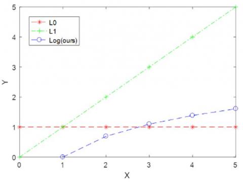
The distributions of rank function, l1 function, and log function were compared to further explain the different approximation effects.
Figure 1. Comparison of rank function, l1 function, and log function
As shown in Figure 1, log function fell between rank function and l1 norm, which can simultaneously increase the penalty on small values and decrease the penalty on large values.
Next, the DCA mentioned in Subsection 2.3 was employed to solve model (26).
Let $f(\chi)=\Phi(\chi)+\frac{1}{2 \mu}\|\mathcal{A}(\chi)-\mathrm{b}\|_{2}^{2}$. Then model (26) can be expressed as:
$\min \{f(\chi):=g(\chi)-h(\chi)\}$ (27)
where, $\chi \in R^{n_{1} \times n_{2} \times \cdots n_{N}}$. The DC components g(X) and h(X) can be respectively given by:
$g(\chi)=\frac{1}{2 \mu}\|\mathcal{A}(X)-\mathrm{b}\|_{2}^{2}+\|\mathcal{X}\|_*$ (28)
where, λ≥0 is a parameter; and
$h(\chi)=\|\chi\|_{*}-\Phi(\chi)$ (29)
According to Subsection 2.3, the DCA scheme for model (27) was determined by computing the two sequences {Xk} and {Yk} which satisfy the following conditions:
$y^{k} \in \partial h\left(\chi^{k}\right), x^{k+1} \in \partial g^{*}\left(y^{k}\right)$ (30)
The calculation process of ∂h(Xk) and ∂g*(Yk) will be repeated in the following subsections.
3.1 Calculation of ∂h(Xk)
From the previous discussion, we have:
$h\left(\chi^{k}\right)=\left\|\chi^{k}\right\|_{*}-\Phi\left(\chi^{k}\right)=\sum_{i=1}^{N}\left(\alpha_{i}\left\|X_{(i)}^{k}\right\|_{*}\right.-$$\left.\varphi\left(X_{(i)}^{k}\right)\right)$ (31)
where, $\Phi(\chi)=\sum_{i=1}^{N} \varphi\left(X_{(i)}\right)$; $\varphi(\mathrm{X})=\sum_{j=1}^{n} \log \left(\sigma_{j}\left(X_{(i)}\right)+\varepsilon\right)$. Then, the subdifferential of h(Xk) is:
$\partial h\left(X^{k}\right)=\sum_{i=1}^{N} \partial\left(\alpha_{i}\left\|X_{(i)}^{k}\right\|_{x}-\varphi\left(X_{(i)}^{k}\right)\right)=$$\sum_{i=1}^{N}\left(\alpha_{i} \partial f_{1} \circ \sigma\left(X_{(i)}^{k}\right)-\partial f_{2} \circ \sigma\left(X_{(i)}^{k}\right)\right)$ (32)
where, σ(X) denotes is the vector consisting of the singular values of matrix X, and ∀x∈Rn: $f_{1}(x)=\sum_{i=1}^{n} x_{i}$ and $f_{2}(x)=\sum_{i=1}^{n} \log \left(x_{i}+\epsilon\right)$.
By Theorem 2.1, we have:
$Y \in \partial(f \circ \sigma)(X)=$$\left\{U(\operatorname{Diag} \omega) V^{T} | \omega \in \partial f(\sigma(X)), X=U(\operatorname{Diag} \sigma(X)) V^{T}\right\}$ (33)
Thereby, following conclusion can be drawn:
$U\left(\begin{array}{cccc}\alpha_{i} & 0 & 0 & 0 \\ 0 & \alpha_{i} & 0 & 0 \\ 0 & 0 & \ddots & 0 \\ 0 & 0 & 0 & \alpha_{i}\end{array}\right)_{r_{i} \times r_{i}} V^{T} \in \alpha_{i} \partial f_{1} \circ \sigma\left(X_{(i)}^{k}\right)$ (34)
and
$U\left(\begin{array}{cccc}\frac{1}{\sigma_{1}\left(x_{(i)}^{k}\right)+\varepsilon} & 0 & 0 & 0 \\ 0 & \frac{1}{\sigma_{2}\left(x_{(i)}^{k}\right)+\varepsilon} & 0 & 0 \\ 0 & 0 & \ddots & 0 \\ 0 & 0 & 0 & \frac{1}{\sigma_{r_{i}}\left(x_{(i)}^{k}\right)+\varepsilon}\end{array}\right)_{r_{i} \times r_{i}}$ $V^{T} \in \partial f_{2} \circ \sigma\left(X_{(i)}^{k}\right)$ (35)
where, ri is the rank of matrix $X_{(i)}^{k}$. Therefore, an element Yk could be found in ∂h(Xk) which has the following form:
$\mathcal{Y}^{k}=\frac{1}{N} \sum_{i=1}^{N} f o l d M_{i}$ (36)
where,
$M_{i}=U\left(\begin{array}{cccc}\alpha_{i}-\frac{1}{\sigma_{1}\left(x_{(i)}^{k}\right)+\varepsilon} & 0 & 0 & 0 \\ 0 & \alpha_{i}-\frac{1}{\sigma_{2}\left(x_{(i)}^{k}\right)+\varepsilon} & 0 & 0 \\ 0 & 0 & \ddots & 0 \\ 0 & 0 & 0 & \alpha_{i}-\frac{1}{\sigma_{r_{i}}\left(x_{(i)}^{k}\right)+\varepsilon}\end{array}\right) V^{T}$ (37)
3.2 Calculation of ∂g*(Yk)
According to the preliminary knowledge in Subsection 2.3, ∂g*(Yk) is a solution to the convex program (22). $\forall \mathcal{Y}^{k} \in R^{n_{1} \times n_{2} \times \cdots n_{N}}$,
$\begin{aligned} \partial g^{*}\left(\mathcal{Y}^{k}\right) &=\arg \min \left\{g(\mathcal{X})-h\left(\mathcal{X}^{k}\right)-<\mathcal{X}-\mathcal{X}^{k}, \mathcal{Y}^{k}>: \mathcal{X} \in R^{n_{1} \times n_{2} \times \cdots n_{N}}\right\} \\ &=\arg \min \left\{g(\mathcal{X})-<\mathcal{X}-\mathcal{X}^{k}, \mathcal{Y}^{k}>: X \in R^{n_{1} \times n_{2} \times \cdots n_{N}}\right\} \end{aligned}$ (38)
Combining (28) and (38), the following optimization can be obtained:
$\min \frac{1}{2 \mu}\|\mathcal{A}(\mathcal{X})-\mathrm{b}\|_{2}^{2}+\|\mathcal{X}\|_{*}-<\mathcal{X}-\mathcal{X}^{k}, y^{k}>, y^{k} \in \partial h\left(\mathcal{X}^{k}\right)$ (39)
Since the optimal condition for minimization of a convex function is 0∈∂φ(x), $\mathcal{X}^{*}$ is optimal of formula (39) if and only if
$0 \in \frac{1}{\mu} \mathrm{P}\left(\mathcal{X}^{*}\right)+\partial\|\mathcal{X}\|_{*}-\mathcal{Y}^{k}$ (40)
where, $\mathrm{P}\left(\mathcal{X}^{*}\right)=\mathcal{A}^{*}\left(\mathcal{A}\left(\mathcal{X}^{*}\right)-\mathrm{b}\right)$ and $\mathcal{A}^{*}$ represents the adjoint of $\mathcal{A}$.
For ∀τ>0, formula (40) is equivalent to:
$0 \in \frac{1}{\mu} \tau P\left(\mathcal{X}^{*}\right)+\tau \partial\|\mathcal{X}\|_{*}-\tau \mathcal{Y}^{k}+\frac{1}{\mu} \mathcal{X}^{*}-\frac{1}{\mu} \mathcal{X}^{*}$ (41)
Then, it holds that
$0 \in \tau \partial\|\mathcal{X}\|_{*}+\frac{1}{\mu} \mathcal{X}^{*}-\frac{1}{\mu}\left(\mathcal{X}^{*}-\tau \mathrm{P}\left(\mathcal{X}^{*}\right)\right)-\tau y^{k}$ (42)
Let $\mathcal{Z}^{*}=\mathcal{X}^{*}-\tau \mathrm{P}\left(\mathcal{X}^{*}\right)$. Formula (42) can be reduced to:
$0 \in \tau \partial\|\mathcal{X}\|_{*}+\frac{1}{\mu} \mathcal{X}^{*}-\frac{1}{\mu}\mathcal{Z}^{*}-\tau y^{k}$ (43)
After combining, we have:
$0 \in \tau \partial\|\mathcal{X}\|_{*}+\frac{1}{\mu}\left(\mathcal{X}^{*}-\left(\mathcal{Z}^{*}+\mu \tau \mathcal{Y}^{k}\right)\right)$ (44)
i.e. $\mathcal{X}^{*}$ is the optimal solution to
$\min \tau\|\mathcal{X}\|_{*}+\frac{1}{2 \mu}\left\|\mathcal{X}-\left(\mathcal{Z}^{*}+\mu \tau \mathcal{Y}^{k}\right)\right\|_{F}^{2}$ (45)
Under the definition of mode-n unfolding, the problem of minimizing (45) can be written as:
$\min \tau \sum_{i=1}^{N} \alpha_{i}\left\|X_{(i)}\right\|_{*}+\frac{1}{2 N \mu} \sum_{i=1}^{N} \| X_{(i)}-\left(Z_{(i)}^{*}+\right.$$\left.\mu \tau Y_{(i)}^{k}\right) \|_{F}^{2}$ (46)
Problem (46) is difficult to solve due to the interdependent nuclear norms. Therefore, a series of new matrix variables Mi (i=1, 2, ..., N) were introduced such that they equal to X(1), X(2), ..., X(N), respectively, which represent the different mode-n unfoldings of the tensor X. With these new variables, formula (46) can be rewritten as:
$\min \tau \sum_{i=1}^{N} \alpha_{i}\left\|M_{i}\right\|_{*}+\frac{1}{2 N \mu} \sum_{i=1}^{N} \| M_{i}-\left(\mathrm{Z}_{(i)}^{*}+\right.$$\left.\mu \tau \mathrm{Y}_{(i)}^{k}\right) \|_{F}^{2}$ s.t. $M_{i}=X_{(i)}, \forall i \in\{1,2, \cdots, N\}$ (47)
Relaxing the constraint Mi=X(i), the following problem can be obtained:
$\min \tau \sum_{i=1}^{N} \alpha_{i}\left\|M_{i}\right\|_{*}+\frac{1}{2 N \mu} \sum_{i=1}^{N} \| M_{i}-\left(\mathrm{Z}_{(i)}^{*}+\right.$$\left.\mu \tau \mathrm{Y}_{(i)}^{k}\right)\left\|_{F}^{2}+\frac{1}{2 \beta} \sum_{i=1}^{N}\right\| M_{i}-X_{(i)} \|_{F}^{2}$ (48)
where, β>0 is a penalty parameter. An optimal solution of problem (48) approaches an optimal solution of formula (47) as β>0 [42]. For convenience, suppose β=μ in problem (48) and consider the following minimization:
$\min _{x, M_{i}} \tau \sum_{i=1}^{N} \alpha_{i}\left\|M_{i}\right\|_{*}+\frac{1}{2 N \mu} \sum_{i=1}^{N} \| M_{i}-\left(\mathrm{Z}_{(i)}^{*}+\right.$$\left.\mu \tau \mathrm{Y}_{(i)}^{k}\right)\left\|_{F}^{2}+\frac{1}{2 \mu} \sum_{i=1}^{N}\right\| M_{i}-X_{(i)} \|_{F}^{2}$ (49)
Computing Mi Fixing all variables except Mi (i=1, 2, ..., N), problem (49) can be transformed into the following matrix problem:
$\min _{M_{i}} \tau \alpha_{i}\left\|M_{i}\right\|_{*}+\frac{1}{2 N \mu}\left\|M_{i}-\left(Z_{(i)}^{*}+\mu \tau Y_{(i)}^{k}\right)\right\|_{F}^{2}+$$\frac{1}{2 u}\left\|M_{i}-X_{(i)}\right\|_{F}^{2}$ (50)
The optimal solution of problem (50) will be searched for by the following theorem.
Theorem 3.1 Suppose μ>0 and τ>0. For any given i∈{1, 2, ..., N}, $M_{i}^{*}$ is an optimal solution to problem (50) if and only if
$M_{i}^{*}=D_{\frac{\tau \alpha_{i} \mu N}{1+N}}\left(\frac{Z_{(i)}^{*}+\mu \tau Y_{(i)}^{k}+N X_{(i)}}{1+N}\right)$ (51)
Proof: $M_{i}^{*}$ is an optimal solution to problem (50) if and only if
$0 \in \partial \tau \alpha_{i}\left\|M_{i}^{*}\right\|_{*}+\frac{1}{N \mu}\left(M_{i}^{*}-\left(\mathrm{Z}_{(i)}^{*}+\mu \tau \mathrm{Y}_{(i)}^{k}\right)\right)+$$\frac{1}{\mu}\left(M_{i}^{*}-X_{(i)}\right)$ (52)
where, $\partial\left\|M_{i}^{*}\right\|_*$ is the subgradients of $\|\cdot\|_{*}$ at $M_{i}^{*}$. Through proper combining and deforming, we have:
$0 \in \partial \frac{\tau \alpha_{i}}{\frac{1+N}{\mu N}}\left\|M_{i}^{*}\right\|_{*}+M_{i}^{*}-\frac{\frac{1}{\mu N}}{\frac{1+N}{\mu N}}\left(\mathrm{Z}_{(i)}^{*}+\mu \tau \mathrm{Y}_{(i)}^{k}\right)-$$\frac{\frac{1}{\mu}}{\frac{1+N}{\mu N}} X_{(i)}$ (53)
which is equivalent to
$0 \in \partial \frac{\tau \alpha_{i} \mu N}{1+N}\left\|M_{i}^{*}\right\|_{*}+M_{i}^{*}-\frac{1}{1+N}\left(\mathrm{Z}_{(i)}^{*}+\right.$$\left.\mu \tau Y_{(i)}^{k}+N X_{(i)}\right)$ (54)
i.e. $M_{i}^{*}$ is an optimal solution to the following minimization problem
$\min \frac{\tau \alpha_{i} \mu N}{1+N}\left\|M_{i}\right\|_{*}+\frac{1}{2} \| M_{i}-\frac{1}{1+N}\left(\mathrm{Z}_{(i)}^{*}+\right.$$\left.\mu \tau Y_{(i)}^{k}+N X_{(i)}\right) \|_{F}^{2}$ (55)
According to the Theorem 3 in Ma et al. [43], an optimal solution to problem (55) must be the matrix shrinkage operator applied to $\frac{1}{1+N}\left(\mathrm{Z}_{(i)}^{*}+\mu \tau \mathrm{Y}_{(i)}^{k}+N X_{(i)}\right)$. Hence, the optimal solution of problem (55) is
$M_{i}^{*}=D_{\frac{\tau \alpha_{i} \mu N}{1+N}}\left(\frac{\mathrm{Z}_{(i)}^{*}+\mu \tau \mathrm{Y}_{(i)}^{k}+N X_{(i)}}{1+N}\right)$ (56)
For ∀νÎR+, the matrix shrinkage operator Dv(X) can be defined as:
$D_{v}(X)=U \operatorname{Diag}(\bar{\sigma}(X)) V^{T}$ (57)
Let $X=\operatorname{UDiag}(\sigma(X)) V^{T}$ be the SVD for matrix X,
$\bar{\sigma}(X)=\left\{\begin{array}{cl}\sigma_{i}(X)-v, & \text { if } \sigma_{i}(X)-v>0 \\ 0, & 0 . W\end{array}\right.$ (58)
Then, solution (56) is also the optimal solution to problem (50).
Q.E.D.
Computing X: Fixing all other variables except X(i), i=1, 2, ..., N, the following problem was considered to get the exact solution:
$\min \frac{1}{2 \mu}\left\|M_{i}-X_{(i)}\right\|_{F}^{2}$ s.t. $X_{(i)}^{*}=M_{i}$ (59)
From the previous discussion, Mi can be regarded as known in model (59). Hence, the solution to model (59) can be obtained easily as:
$\chi^{*}=\frac{1}{N} \sum_{i=1}^{N} f o l d\left(M_{i}\right)$ (60)
From formulas (56) and (60), the following iterative formula can be derived:
$\left\{\begin{array} & Y^k_{(i)}=U\left(\begin{array}{ccc}\alpha_{i}-\frac{1}{\sigma_{1}\left(x_{(i)}^{k}\right)+\varepsilon} & 0 & 0 & 0 \\ 0 & \alpha_{i}-\frac{1}{\sigma_{2}\left(x_{(i)}^{k}\right)+\varepsilon} & 0 & 0 \\ 0 & 0 & \ddots & 0 \\ 0 & 0 & 0 & \alpha_{i}-\frac{1}{\sigma_{r_{i}}\left(x_{(i)}^{k}\right)+\varepsilon}\end{array}\right)V^T \\ Z_{(i)}^{k}=\chi^{k}-\tau \mathrm{P}\left(\chi^{k}\right) & & \\ \chi^{k+1}=\frac{1}{N} \sum_{i=1}^{N} f \text { old } D_{\frac{\tau \alpha_{i} \mu N}{1+N}}\left(\frac{\mathrm{z}_{(i)}^{k}+\mu \tau \mathrm{Y}_{(i)}^{k}+N X_{(i)}}{1+N}\right) & & \end{array}\right.$ (61)
Through the above discussion, the Log-TC algorithm can be established to solve tensor completion problem (Algorithm 1).
|
Algorithm 1: Log-TC algorithm |
|
Input: $\mathcal{A}$, b, $\mu$, and $\tau$ Initialization: Set k:=0, and $\chi^{k}:=0$ for μ→0, do while not converged, do P($$\chi^{k}$)=$\mathcal{A}^{*}\left(\mathcal{A}\left(\mathcal{X}^{*}\right)-b\right)$ $z^{k}=\chi^{k}-\tau P\left(\chi^{k}\right)$ for i = 1:N $M_{i}^{k}=D_{\frac{\tau \alpha_{i} \mu N}{1+N}}\left(\frac{Z_{(i)}^{k}+\mu \tau Y_{(i)}^{k}+N X_{(i)}}{1+N}\right)$ end $\chi^{k+1}=\frac{1}{N} \sum_{i=1}^{N} f o l d\left(M_{i}^{k}\right)$ end while end for Output: $\chi_{u l t}$ |
To verify its empirical performance, the proposed Log-TC algorithm was compared with fixed point iterative method for low-rank tensor completion (FP-LRTC) [44] and fast low rank tensor completion algorithm (FaLRTC) [10] through numerical experiments. The FP-LRTC, which combines a fixed-point iterative method for solving the low n-rank tensor pursuit problem, and a continuation technique, has been applied to solve the relaxation model of the low-rank tensor completion problem. The FaLRTC utilizes a smoothing scheme to transform the original nonsmooth problem into a smooth problem, and was found more efficient than simple low rank tensor completion (SiLRTC), and high accuracy low rank tensor completion (HaLRTC).
This section is separated into two subsections. In Subsection 4.1, our algorithm was tested on the randomly generated low n-rank tensors. In Subsection 4.2, our algorithm was tested on color image recovery problem. All experiments were carried out in MATLAB R2016a on a computer running on Windows 10, with a 3.20GHz CPU and 4GB of memory. For fair comparison, each number is the average over 10 separate runs.
4.1 Synthetic data
First, our Log-TC algorithm was tested on several synthetic datasets for the tensor completion tasks. Following the method proposed by Rauhut et al. [45], a n-order tensor $\mathcal{J} \in R^{n_{1} \times n_{2} \times \cdots \times n_{N}}$ was created randomly with the n-rank (r1, r2, ..., rN) of the form $\mathcal{T}:=\mathcal{M} \times_{1} U_{1} \times_{2} \cdots \times_{N} U_{N}$, where $\mathcal{M} \in R^{r_{1} \times r_{2} \times \cdots \times r_{N}}$ is the core tensor and $U_{i} \in R^{n_{i} \times r_{i}}(i=1,2, \cdots, N)$. Each entry of the core tensor $\mathcal{M}$ was sampled independently from a standard Gaussian distribution $\mathcal{N}(0,1)$. Then, m entries were sampled randomly from tensor $\mathcal{T}$ in a uniform manner. The sample ratio, denoted by SR, was defined as $\mathrm{SR}=m / I_{1} \cdots I_{N}$. The relative error (RelErr) of the recovered tensor defined as:
$\operatorname{Rel} \mathrm{Err}=\frac{\left\|x_{u l t}-\mathcal{T}\right\|_{F}}{\|\mathcal{T}\|_{F}}$ (62)
is used to estimate the closeness of $x_{u l t}$ to $\mathcal{T}$, where $x_{u l t}$ is the optimal solution to model (26) produced by the algorithms.
The ratio “fr” [44] between the degree of freedom (DOF) in a rank r matrix to the number of samples in the matrix completion was extended to tensor completion problem and denoted by FR:
$\mathrm{FR}=\frac{1}{N} \sum_{i=1}^{N} f r_{i}=\frac{1}{N} \sum_{i=1}^{N} \frac{r_{i}\left(I_{i}+\Pi_{i}-r_{i}\right)}{I_{1} \cdots I_{N} \times S R}$ (63)
where, $r_{i}=\operatorname{rank}\left(X_{(i)}\right)$; $\Pi_{i}=\prod_{k=1, k \neq i}^{N} I_{k}$. In the following results, “FR” is used to represent the hardness of the tensor completion. If FR is greater than 0.6, then the problems are “hard problems”; otherwise, the problems are “easy problems”. The parameters wee configured as: μ=1, θμ=1-sr, $\bar{\mu}=$$1 \times 10^{-8}$, τ=10, and λ=1.
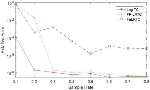
The simulated performance of FP-LRTC, FaLRTC and Log-TC for random tensor completion problem, as measured by relative error and running time, are reported in Figure 2 and Table 1.
As shown in Figure 2, the relative error for tensor of size 60×60×60 with the n-rank was fixed at (6,6,6), and the sample rate changed from 10% to 80%. As it is known, when the n-rank is fixed, the complexity of the problem increases with the decrease of the SR. The plot illustrates that Log-TC is clearly superior to FP-LRTC and FaLRTC. The superiority is particularly evidence in the situation of SR=10%: Log-TC recovered the tensor with the relative error about 10-4, while FaLRTC and FP-LRTC with 100.
Figure 2. The relative error on tensors of size 60×60×60 with sample rate (SR) between 10% to 80% and fixed n-rank (6,6,6)
Table 1. Comparison of running time on tensors of size 60×60×60 with sample rate (SR) 70% and -rank (6,6,6)
|
Relative Error |
Log-TC Time (s) |
FP-LRTC Time (s) |
FaLRTC Time (s) |
|
$10^{-9}$ |
67.23 |
79.04 |
132.41 |
|
$10^{-8}$ |
26.62 |
32.75 |
40.42 |
|
$10^{-6}$ |
11.07 |
16.36 |
36.21 |
|
$10^{-4}$ |
2.82 |
4.51 |
41.17 |
Table 1 shows the performance of each algorithm with SR 70% in terms of the running time. Log-TC obviously outperformed the contrastive algorithms, under the same relative error. Even when the precision requirement is ultrahigh (10-9), Log-TC can complete the trask in one minute.
Figure 3 shows the relative error for tensor of size 60×60×60, when the sample rate was fixed at SR=40% and n-rank r changed from 2 to 40. Like the previous situation, when sample rate is fixed, the complexity of the problem increases with the increase of the rank. As shown in Figure 3, Log-TC outperformed FP-LRTC and FaLRTC in all cases. Log-TC performed especially well at r=20: Log-TC recovered the tensors with the relative error about 10-8, while FP-LRTC and FaLRTC with only about 10-1. It can also be seen that, when r=24, our algorithm solved the problem with the relative error 10-3, but the other two methods failed to effectively recover the tensors.
Figure 3. The relative error on tensors of size 60×60×60 n-rank (r,r,r) between 2 and 40 and fixed sample rate (SR=40%).
Next, the numerical results of the three algorithms on easy problems and hard problems were reported. Tables 2 and 3 list the numerical results of several cases in which the test tensors have different sizes, n-ranks and sample rates.
According to the results on easy problems (Table 2), the Log-TC outshined the other two algorithms in relative error and running time. FaLRTC is inferior to FP-LRTC and Log-TC in terms of relative error. FP-LRTC and Log-TC performed similarly on relative error, but Log-TC consumed the shorter time. Overall, Log-TC achieved the best performance on easy problems.
According to the results on hard problems (Table 3), Log-TC also realized better performance than the contrastive algorithms. With the increase of tensor order, the robustness of FaLRTC was getting worse. FP-LRTC and Log-TC were always capable of recovering the tensors efficiently, but the running time of FP-LRTC is about 2.5 times more than that of the Log-TC.
Table 2. Comparison results for easy problems
|
Tensor |
Rank |
SR |
FR |
Log-TC |
FP-LRTC |
FaLRTC |
|||
|
RelErr |
Time |
RelErr |
Time |
RelErr |
Time |
||||
|
20×30×40 |
(2,2,2) |
0.5 |
0.15 |
1.72e-08 |
1.11 |
3.36e-08 |
1.82 |
1.23e-06 |
3.53 |
|
30×30×30 |
(5,5,5) |
0.3 |
0.57 |
5.42e-08 |
3.24 |
8.27e-07 |
4.39 |
4.83e-06 |
2.72 |
|
60×60×60 |
(5,5,5) |
0.7 |
0.12 |
4.57e-09 |
2.83 |
6.71e-09 |
4.65 |
1.11e-05 |
7.88 |
|
100×100×100 |
(10,10,10) |
0.4 |
0.25 |
3.95e-09 |
50.40 |
5.90e-09 |
87.28 |
1.21e-05 |
36.63 |
|
20×20×30×30 |
(5,5,5,5) |
0.6 |
0.35 |
4.40e-09 |
13.57 |
5.76e-09 |
22.87 |
5.94e-07 |
90.76 |
|
50×50×50×50 |
(6,6,6,6) |
0.7 |
0.17 |
1.23e-09 |
90.77 |
1.64e-09 |
139.19 |
2.36e-08 |
189.6 |
|
30×30×30×30×30 |
(2,2,2,2,2) |
0.5 |
0.13 |
1.83e-09 |
635.81 |
2.44e-09 |
1573.9 |
9.83e-08 |
2896 |
|
30×30×30×30×30 |
(6,6,6,6,6) |
0.6 |
0.33 |
1.43e-09 |
905.60 |
1.47e-09 |
1649.1 |
8.63e-08 |
2765 |
Table 3. Comparison results for hard problems
|
Tensor |
Rank |
SR |
FR |
Log-TC |
FP-LRTC |
FaLRTC |
|||
|
RelErr |
Time |
RelErr |
Time |
RelErr |
Time |
||||
|
20×30×40 |
(2,2,2) |
0.1 |
0.75 |
3.90e-04 |
50.82 |
5.72e-01 |
67.61 |
2.11e-01 |
6.73 |
|
30×30×30 |
(5,5,5) |
0.1 |
1.71 |
8.30e-10 |
57.83 |
8.45e-7 |
62.09 |
8.74e-01 |
1.31 |
|
70×70×70 |
(10,10,10) |
0.2 |
0.72 |
2.28e-08 |
324.83 |
2.71e-08 |
422.34 |
2.35e-04 |
56.42 |
|
100×100×100 |
(10,10,10) |
0.2 |
0.63 |
1.20e-08 |
119.29 |
1.67e-08 |
187.10 |
1.09e-04 |
191.5 |
|
20×20×30×30 |
(5,5,5,5) |
0.3 |
0.7 |
1.34e-08 |
241.36 |
4.76e-07 |
373.09 |
3.42e-07 |
896.3 |
|
50×50×50×50 |
(5,5,5,5) |
0.2 |
0.69 |
7.18e-09 |
754.08 |
5.43e-08 |
1271.51 |
2.72e-01 |
1732 |
|
20×20×20×20×20 |
(5,5,5,5,5) |
0.3 |
0.83 |
3.04e-08 |
398.47 |
6.28e-06 |
1689.23 |
3.92e-01 |
2874 |
|
20×20×20×20×20 |
(8,8,8,8,8) |
0.4 |
1.00 |
4.48e-09 |
746.92 |
8.52e-08 |
1939.63 |
4.53e-08 |
2145 |
4.2 Image simulation
This subsection compared the three algorithms on the recovery of color images. Color images can be expressed as third order tensors. If the images are of low rank, the image recovery can be solved as a low n-rank tensor completion problem. Assuming that the images are well structured, FP-LRTC, FaLRTC and Log-TC were applied separately to solve the recovery problem.
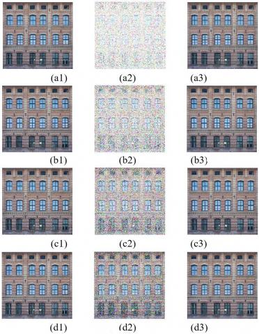
The recovery effects of the Log-TC are illustrated in Figure 4 and Table 4. In Figure 4, (a1), (b1), (c1), and (d1) are original color images. Then, 80%, 60%, 40% and 20% entries were randomly removed, creating corrupted images (a2), (b2), (c2), and (d2), respectively. The images recovered by the Log-TC are (a3), (b3), (c3), and (d4), respectively. Only the effects of the Log-TC were provided, because the three algorithms achieved similar recovery accuracy. The recovery accuracy and running time of each algorithm are listed in Table 4.
Figure 4. Original images, corrupted images, and recovered image by Log-TC in the recovery of natural images
Table 4. Numerical results on the color images
|
SR |
Log-TC |
FP-LRTC |
FaLRTC |
|||
|
Relative Error |
Time (s) |
Relative Error |
Time (s) |
Relative Error |
Time (s) |
|
|
20% |
9.14e-02 |
1300 |
9.62e-02 |
1681 |
8.31e-02 |
2137 |
|
40% |
6.36e-02 |
598 |
8.45e-02 |
740 |
7.74e-02 |
1402 |
|
60% |
4.89e-02 |
362 |
5.71e-02 |
298 |
2.57e-02 |
978 |
|
80% |
3.40e-02 |
209 |
4.21e-02 |
302 |
3.91e-02 |
721 |
As shown in Figure 4, the Log-TC recovered the natural images with missing information. Table 4 shows that our algorithm achieved a recovery accuracy of about 10-2, and a clear edge over the contrastive methods in running time.
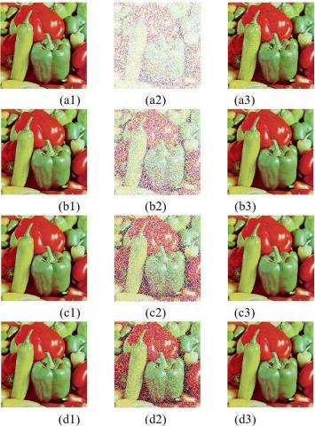
Figure 5. Original images, corrupted images, recovered images by the Log-TC in the recovery of images with poor texture
Table 5. Numerical results on the color image with poor texture
|
SR |
Log-TC |
FP-LRTC |
FaLRTC |
|||
|
Relative Error |
Time(s) |
Relative Error |
Time(s) |
Relative Error |
Time(s) |
|
|
20% |
1.17e-01 |
1835 |
5.72e-01 |
1920 |
4.53e-01 |
2341 |
|
40% |
6.71e-02 |
857 |
8.45e-02 |
1103 |
7.47e-02 |
1780 |
|
60% |
5.02e-02 |
493 |
2.71e-02 |
631 |
3.87e-02 |
1285 |
|
80% |
3.37e-02 |
291 |
4.42e-02 |
329 |
2.57e-02 |
943 |
This paper firstly defines a log function of tensor, and uses it as an approximation of tensor rank function. Furthermore, a simple yet efficient algorithm named Log-TC algorithm was proposed to recover an underlying low n-rank tensor. The log function strikes a balance between rank minimization and nuclear norm. It can simultaneously increase the penalty on small values and reduce the penalty on large values. After that, our algorithm was compared with FP-LRTC and FaLRTC through numerical experiments on randomly generated tensors and color image recovery. The numerical comparisons demonstrate that the Log-TC outperformed the other two algorithms. The future research will investigate the largescale cases by other techniques, and test the performance of our algorithm for image inpainting problems.
The authors would like to thank the anonymous reviewers for the useful comments and suggestions. This work is partially supported by National Natural Science Foundation of China Grant (No. 11626080), Natural Science Foundation of Hebei Province (No. A2017207011), National Statistical Science Research Project of China (No. 2019LY27) and Department of Education of Hebei Province under Grant (No. QN2018018).
[1] Symeonidis, P. (2016). Matrix and tensor decomposition in recommender systems. In Proceedings of the 10th ACM Conference on Recommender Systems, pp. 429-430. https://doi.org/10.1145/2959100.2959195
[2] Peng, J., Zeng, D.D., Zhao, H., Wang, F.Y. (2010). Collaborative filtering in social tagging systems based on joint item-tag recommendations. In Proceedings of the 19th ACM International Conference on Information and Knowledge Management, pp. 809-818. https://doi.org/10.1145/1871437.1871541
[3] Xiong, L., Chen, X., Huang, T.K., Schneider, J., Carbonell, J.G. (2010). Temporal collaborative filtering with Bayesian probabilistic tensor factorization. In Proceedings of the 2010 SIAM International Conference on Data Mining, pp. 211-222. https://doi.org/10.1137/1.9781611972801.19
[4] Baltrunas, L., Kaminskas, M., Ludwig, B., Moling, O., Ricci, F., Aydin, A., Lüke, K.H., Schwaiger, R. (2011). Incarmusic: Context-aware music recommendations in a car. In International Conference on Electronic Commerce and Web Technologies, pp. 89-100. https://doi.org/10.1007/978-3-642-23014-1_8
[5] Cichocki, A., Mandic, D., De Lathauwer, L., Zhou, G., Zhao, Q., Caiafa, C., Phan, H.A. (2015). Tensor decompositions for signal processing applications: From two-way to multiway component analysis. IEEE Signal Processing Magazine, 32(2): 145-163. https://doi.org/10.1109/MSP.2013.2297439
[6] Cichocki, A., Lee, N., Oseledets, I., Phan, A.H., Zhao, Q., Mandic, D.P. (2016). Tensor networks for dimensionality reduction and large-scale optimization: Part 1 low-rank tensor decompositions. Foundations and Trends® in Machine Learning, 9(4-5): 249-429. https://doi.org/10.1561/2200000059
[7] Cichocki, A., Phan, A.H., Zhao, Q., Lee, N., Oseledets, I.V., Sugiyama, M., Mandic, D. (2017). Tensor networks for dimensionality reduction and large-scale optimization: Part 2 applications and future perspectives. Foundations and Trends R in Machine Learning, 9(6): 431-673. https://doi.org/10.1561/2200000067
[8] Sidiropoulos, N.D., De Lathauwer, L., Fu, X., Huang, K., Papalexakis, E.E., Faloutsos, C. (2017). Tensor decomposition for signal processing and machine learning. IEEE Transactions on Signal Processing, 65(13): 3551-3582. https://doi.org/10.1109/TSP.2017.2690524
[9] Signoretto, M., Van de Plas, R., De Moor, B., Suykens, J. A. (2011). Tensor versus matrix completion: A comparison with application to spectral data. IEEE Signal Processing Letters, 18(7): 403-406. https://doi.org/10.1109/LSP.2011.2151856
[10] Liu, J., Musialski, P., Wonka, P., Ye, J. (2012). Tensor completion for estimating missing values in visual data. IEEE Transactions on Pattern Analysis and Machine Intelligence, 35(1): 208-220. https://doi.org/10.1109/TPAMI.2012.39
[11] Wang, W., Sun, Y., Eriksson, B., Wang, W., Aggarwal, V. (2018). Wide compression: Tensor ring nets. In Proceedings of the IEEE Conference on Computer Vision and Pattern Recognition, pp. 9329-9338.
[12] He, W., Yuan, L., Yokoya, N. (2019). Total-variation-regularized tensor ring completion for remote sensing image reconstruction. In ICASSP 2019-2019 IEEE International Conference on Acoustics, Speech and Signal Processing (ICASSP), Brighton, United Kingdom, United Kingdom, pp. 8603-8607. https://doi.org/10.1109/ICASSP.2019.8682696
[13] Huang, H., Liu, Y., Liu, J., Zhu, C. (2020). Provable tensor ring completion. Signal Processing, 171: 107486. https://doi.org/10.1016/j.sigpro.2020.107486
[14] Liu, Y., Shang, F., Jiao, L., Cheng, J., Cheng, H. (2014). Trace norm regularized CANDECOMP/PARAFAC decomposition with missing data. IEEE transactions on cybernetics, 45(11): 2437-2448. https://doi.org/10.1109/TCYB.2014.2374695
[15] Jenatton, R., Roux, N.L., Bordes, A., Obozinski, G.R. (2012). A latent factor model for highly multi-relational data. In Advances in neural information processing systems, pp. 3167-3175.
[16] Guo, X., Yao, Q., Kwok, J.T.Y. (2017). Efficient sparse low-rank tensor completion using the Frank-Wolfe algorithm. In Thirty-First AAAI Conference on Artificial Intelligence.
[17] Sorber, L., Van Barel, M., De Lathauwer, L. (2013). Optimization-based algorithms for tensor decompositions: Canonical polyadic decomposition, decomposition in rank-(Lr, Lr, 1) terms, and a new generalization. SIAM Journal on Optimization, 23(2): 695-720. https://doi.org/10.1137/120868323
[18] Goulart, J.H.D.M., Boizard, M., Boyer, R., Favier, G., Comon, P. (2015). Tensor CP decomposition with structured factor matrices: Algorithms and performance. IEEE Journal of Selected Topics in Signal Processing, 10(4): 757-769. https://doi.org/10.1109/JSTSP.2015.2509907
[19] Tucker, L.R. (1966). Some mathematical notes on three-mode factor analysis. Psychometrika, 31(3): 279-311. https://doi.org/10.1007/BF02289464
[20] De Lathauwer, L., De Moor, B., Vandewalle, J. (2000). On the best rank-1 and rank-(r1, r2, ..., rN) approximation of higher-order tensors. SIAM Journal on Matrix Analysis and Applications, 21(4): 1324-1342. https://doi.org/10.1137/S0895479898346995
[21] Tsai, C.Y., Saxe, A.M., Cox, D. (2016). Tensor switching networks. In Advances in Neural Information Processing Systems, pp. 2038-2046.
[22] Oseledets, I.V. (2011). Tensor-train decomposition. SIAM Journal on Scientific Computing, 33(5): 2295-2317. https://doi.org/10.1137/090752286
[23] Phien, H.N., Tuan, H.D., Bengua, J.A., Do, M.N. (2016). Efficient tensor completion: Low-rank tensor train. arXiv preprint arXiv:1601.01083.
[24] Yang, Y., Krompass, D., Tresp, V. (2017). Tensor-train recurrent neural networks for video classification. In Proceedings of the 34th International Conference on Machine Learning, 70: 3891-3900. https://doi.org/10.5555/3305890.3306083
[25] Hu, Y., Zhang, D., Ye, J., Li, X., He, X. (2012). Fast and accurate matrix completion via truncated nuclear norm regularization. IEEE Transactions on Pattern Analysis and Machine Intelligence, 35(9): 2117-2130. https://doi.org/10.1109/TPAMI.2012.271
[26] Lu, C., Tang, J., Yan, S., Lin, Z. (2014). Generalized nonconvex nonsmooth low-rank minimization. In Proceedings of the IEEE Conference on Computer Vision and Pattern Recognition, pp. 4130-4137.
[27] Yao, Q., Kwok, J.T., Wang, T., Liu, T.Y. (2018). Large-scale low-rank matrix learning with nonconvex regularizers. IEEE Transactions on Pattern Analysis and Machine Intelligence, 41(11): 2628-2643. https://doi.org/10.1109/TPAMI.2018.2858249
[28] Fan, J., Ding, L., Chen, Y., Udell, M. (2019). Factor group-sparse regularization for efficient low-rank matrix recovery. In Advances in Neural Information Processing Systems, pp. 5105-5115.
[29] Huang, L.T., So, H.C., Chen, Y., Wang, W.Q. (2014). Truncated nuclear norm minimization for tensor completion. In 2014 IEEE 8th Sensor Array and Multichannel Signal Processing Workshop (SAM), pp. 417-420. https://doi.org/10.1109/SAM.2014.6882431
[30] Han, Z.F., Leung, C.S., Huang, L.T., So, H.C. (2017). Sparse and truncated nuclear norm based tensor completion. Neural Processing Letters, 45(3): 729-743. https://doi.org/10.1007/s11063-016-9503-4
[31] Xue, S., Qiu, W., Liu, F., Jin, X. (2018). Low-rank tensor completion by truncated nuclear norm regularization. In 2018 24th International Conference on Pattern Recognition (ICPR), Beijing, China, pp. 2600-2605. https://doi.org/10.1109/ICPR.2018.8546008
[32] Kiers, H.A. (2000). Towards a standardized notation and terminology in multiway analysis. Journal of Chemometrics: A Journal of the Chemometrics Society, 14(3): 105-122. https://doi.org/10.1002/1099-128X(200005/06)14:3%3C105::AID-CEM582%3E3.0.CO;2-I
[33] De Lathauwer, L., De Moor, B., Vandewalle, J. (2000). A multilinear singular value decomposition. SIAM Journal on Matrix Analysis and Applications, 21(4): 1253-1278. https://doi.org/10.1137/S0895479896305696
[34] Lewis, A.S. (1994). The convex analysis of unitarily invariant matrix norms. Faculty of Mathematics, University of Waterloo, 2: 173-183.
[35] Geng, J., Wang, L., Xu, Y., Wang, X. (2014). A weighted nuclear norm method for tensor completion. International Journal of Signal Processing, Image Processing and Pattern Recognition, 7(1): 1-12. http://dx.doi.org/10.14257/ijsip.2014.7.1.01
[36] Han, Z.F., Leung, C.S., Huang, L.T., So, H.C. (2017). Sparse and truncated nuclear norm based tensor completion. Neural Processing Letters, 45(3): 729-743. https://doi.org/10.1007/s11063-016-9503-4
[37] Xue, S., Qiu, W., Liu, F., Jin, X. (2018). Low-rank tensor completion by truncated nuclear norm regularization. In 2018 24th International Conference on Pattern Recognition (ICPR), Beijing, China, pp. 2600-2605. https://doi.org/10.1109/ICPR.2018.8546008
[38] Horst, R., Thoai, N.V. (1999). DC programming: overview. Journal of Optimization Theory and Applications, 103(1): 1-43. https://doi.org/10.1023/A:1021765131316
[39] Le Thi Hoai, A., Tao, P.D. (1997). Solving a class of linearly constrained indefinite quadratic problems by DC algorithms. Journal of Global Optimization, 11(3): 253-285. https://doi.org/10.1023/A:1008288411710
[40] Tao, P.D. (2005). The DC (difference of convex functions) programming and DCA revisited with DC models of real world nonconvex optimization problems. Annals of Operations Research, 133(1-4): 23-46. https://doi.org/10.1007/s10479-004-5022-1
[41] Tao, P.D., An, L.T.H. (1997). Convex analysis approach to DC programming: Theory, algorithms and applications. Acta Mathematica Vietnamica, 22(1): 289-355.
[42] Bertsekas, D.P. (1997). Nonlinear programming. Journal of the Operational Research Society, 48(3): 334-334. https://doi.org/10.1057/palgrave.jors.2600425
[43] Ma, S., Goldfarb, D., Chen, L. (2011). Fixed point and Bregman iterative methods for matrix rank minimization. Mathematical Programming, 128(1-2): 321-353. https://doi.org/10.1007/s10107-009-0306-5
[44] Yang, L., Huang, Z.H., Shi, X. (2013). A fixed point iterative method for low n-rank tensor pursuit. IEEE Transactions on Signal Processing, 61(11): 2952-2962. https://doi.org/10.1109/TSP.2013.2254477
[45] Rauhut, H., Schneider, R., Stojanac, Ž. (2017). Low rank tensor recovery via iterative hard thresholding. Linear Algebra and Its Applications, 523: 220-262. https://doi.org/10.1016/j.laa.2017.02.028