Sufen Zhang
OPEN ACCESS
In recent years, the time dimension of geographic objects has been introduced to the geographic information system (GIS), marking a great progress in geographic information science (GIScience). The mining and knowledge discovery of spatial pattern and spatiotemporal evolution of geographical elements and phenomena have become the hotspot of GIScience research. Based on graph theory, abstract definitions were given to geographical simple objects and composite objects, involving spatial relationships, morphological features and semantic features. These features, attributes and relationships were integrated into a novel relational attribute neighborhood graph (RANG) through the design of a series of algorithms. The RANG was successfully applied to the automatic classification of urban land use, providing a desirable tool for land use classification in the context of rapid urbanization.
geographic information system (GIS), relational attribute neighborhood graph (RANG), graph theory, classification, urban land use
Space, time and attribute are the three inherent features of any geographical element and phenomenon [1]. The three basic features evolve continuously with the constant changes in real-world geography. The dynamic variations of the three features must be considered in the geographic information system (GIS).
Traditionally, the GIS is largely static, focusing only on the spatial features. In recent years, the time dimension has been gradually integrated in the GIS. In this way, the GIS can reflect the changes of geographical elements and phenomena over time, and provide high-quality spatiotemporal information and services, laying the basis for geographical analysis, simulation and prediction.
The GIS integrated with the time dimension can be referred to as the temporal GIS. With the development of the temporal GIS, the spatial data has gradually evolved into spatiotemporal data. The information embedded in spatiotemporal data boasts great application potential in today’s world, as people long to observe, understand and describe geographical phenomena on different spatial and temporal scales.
The temporal GIS and its spatiotemporal data provide a novel solution to many geographical problems, ranging from navigation, traffic control to land use planning. Among them, land use planning, especially in urban areas, is a common concern in many countries. The intensive urban growth in recent decades has brought various problems, calling for better classification of urban land use.
This paper aims to accurately classify urban land use based on graph theory and the GIS. First, the spatiotemporal representation of geographic objects was discussed, revealing the hierarchical structure between composite objects and their lower-level simple objects. Then, the relational attribute neighborhood graph (RANG) was proposed based on the graph theory, involving the semantic, spatial, connectivity and morphological features of land cover elements. Taking land cover elements as simple objects and land use units as composite objects, the RANG and the random forest algorithm were adopted to classify the land use in an urban area.
In geographic information science (GIScience), object-based geospatial expression is a superior way to abstract features and describe semantic meaning of geographic entities and phenomena, thanks to its similarity to human thinking and behavioral patterns [2, 3]. Klien [4] suggested that, based on objects, entities in geo-space could be abstracted into different objects, each of which has its unique behaviors, attributes and rules. Baja et al. [5] held that multiscale features belong to such three levels as geometry, attribute and semantics; therefore, multiple geographic objects could be aggregated into a composite geographic object through different levels of abstraction, depending on their geometric, attribute and semantic features. Lü et al. [6] developed the data structures and models for organizing and expressing the multiscale features of geographic objects.
Besides the GIScience, the object-based methods have also received much attention from scholars engaging in remote sensing. Wang et al. [7] segmented the remote sensing image into a series of objects, and analyzed the objects based on their semantics, spectra and context, revealing that object-based analysis facilitates the interpretation and perception of remote sensing images. Mimicking the image cognition of human brain, Pinheiro et al. [8] combined automatic computer classification with artificial information extraction to segment images of different scales, according to the object information (i.e. hue, shape, texture and level) and the inter-class information (i.e. the features of adjacent objects, sub-objects and parent objects). The combined strategy has been applied in various fields, ranging from urban built-up area extraction, building extraction, to land use classification [9-11].
During object-based image analysis, the target image carries geospatial connotation if its covers part of or all the object in geo-space. Borna et al. [12] developed the geographic object-based image analysis method, and determined the relationship between image objects and geographic objects in the geo-space, in the light of the spatial, spectral and temporal information. Worboys [13] believed that objects have a series of spatial attributes and relationships that can be utilized in image analysis. Mo et al. [14] argued that the image objects should be replaced by the sub-objects, and proposed to establish the hierarchical relationship circularly in image segmentation and classification.
To disclose the hierarchical relationship of objects, researchers have been integrating human cognition and thinking patterns into semantics and ontology in the context of GIScience. For instance, Yue et al. [15] discovered complex geospatial objects based on geospatial semantics and services. Barr and Barnsley [16] designed a region-based extended relational attribute graph structure, and used the structure to express the spatial and semantic relationships between image regions. Starting with the attributes of image objects, Belgiu and Drăguţ [17] identified urban structures with the aid of graph theory and random forest.
The development of remote sensing makes it possible to acquire surface features quickly, giving birth to the concept of land use classification. Gao et al. [18] proposed a four-level land cover classification system, which relies on remote sensing to obtain the attributes of surface features. Wang et al. [19] classified the land cover in China into 22 types, using the SPOT VEGETATION (SPOT/VGT) data with the resolution of 1km. Jansen et al. [20] analyzed the data on land use/cover classification and social statistics, and constructed a land function classification system, which divides land functions into 21 subclasses in 6 classes.
Every geographic object contains information in two dimensions: space and time. Similarly, each geographical phenomenon varies with time and space. To truly understand a geographical phenomenon, it is necessary to fully recognize the spatial and temporal information, and express the two types of information in a unified format.
3.1 Time expression
In geography, time is generally considered as a dimension of spatiotemporal data, and analogized as a straight line linking up the past, present and future. Time exists in three forms: discrete, dense and continuous.
In discrete form, time is described as a sequence of discrete moments: $T=\left\langle T_{1}, T_{2}, \ldots, T_{n}\right\rangle$, where Ti is a moment. In dense form, a moment can be inserted between any two discrete moments. In continuous form, there exists a moment T3 between any two moments T1 and T2 ( $T_{1}<T_{2}$) that satisfy $T_{1}<T_{3}<T_{2}$.
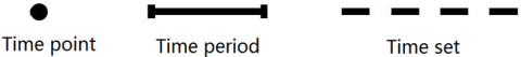
The different forms of time can be expressed by time elements, which are represented by time attributes. Based on time granularity, time elements can be attributed to three categories: time point, time period and time set (Figure 1).
Figure 1. Classification of time elements
The time point, corresponding to the discrete time, is defined as the unit of time obtained when the time is discretized to a certain granularity. The time period refers to an interval $\left\langle T_{i}, T_{j}\right\rangle$ between the start time and the end time. It is often adopted to describe the continuous changes of geographical phenomena. The time set is a union of multiple time periods: $\left\{\left\langle T_{i 1}, T_{j 1}\right\rangle, \ldots,\left\langle T_{i k}, T_{j k}\right\rangle\right\}$. Once the time element is determined, the topological relationship can be defined between different time elements.
3.2 Geographic object
In the visual sense, geographic objects mean the entities, which are larger than a minimum size on the surface, that can be expressed on maps. Typical examples of geographic objects include cities, lakes and mountains. In other words, an object refers to a discrete geographic entity, which is unique in identity and geographically different from the surrounding objects. In object-based data representation, an object is considered as an independent aggregation of the relevant entity features and functions.
The geographic features of an object be represented as a tuple $\left(\mathrm{x}, \mathrm{y}, \mathrm{z}_{1}, \mathrm{z}_{2}, \dots, \mathrm{z}_{n}\right)$, where (x, y) are coordinates, and $Z_{1}, Z_{2}, \dots, Z_{n}$ are attributes. Then, an geographic object can be expressed as $\left(o, a_{1}, a_{2}, \dots, a_{n}\right)$, where o is the object, and $a_{1}, a_{2}, \dots, a_{n}$ are the attributes of the object. On this basis, the geographic object can be formally defined as:
Geographic object(O)=Identity(I)+State(S)+Behavior(B)
where, Identity (I) is a necessary component of geographic object (O) that differentiates it from the other objects in the same area; State (S) describes all the information and conditions of the geographic object at a specific time, including time attributes, spatial attributes and nonspatial attributes; Behavior (B) stands for the changes of the state attributes of the geographic object, such as the shape change.
3.3 Simple object and composite object
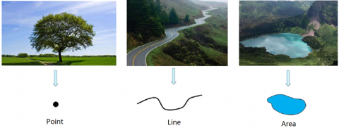
In the geographic world, many entities and phenomena can be expressed with three kinds of simple objects: point, line and area (Figure 2). Together, these three types of simple objects can abstract the same geospatial entity and phenomenon excellently.
Figure 2. Simple geographic objects
Composite objects can be broken down into multiple simple objects. Hence, a composite object can be defined as an object on a superior level to simple objects. All the simple objects belong to the superior composite object.
There are three types of spatial relationships among geographic objects: topological relationship, metric relationship and directional relationship. Topological relationship refers to the connections between geographic objects satisfying the principle of topological geometry, namely, the adjacency, inclusion and connectivity between geographic objects. The topological relationships among geographic objects are often very complex, because the objects are made up differently with points, lines and areas. The measurement relationship describes the link between geographic objects with the measured results in geo-space, including distance and area between the objects. The directional relationship showcases the orientation and sequence of geographic objects in the geo-space.
3.4 Spatial information extraction from composite objects
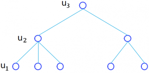
In the GIS, the objects are organized orderly as hierarchies. The complex objects belong to high hierarchies. The sequence between the objects can be expressed as:
$u_{1} \leq u_{2} \quad$ if $f \exists f: u_{2}=f\left\{u_{i}\right\} ; u_{1}=f\left\{u_{i}\right\}$
where, the hierarchy of u1 is lower than that of u2, and u2 can be derived from ui by function f . The orderly structure can be represented by a tree structure (Figure 3).
Figure 3. The orderly hierarchical structure of objects
In the above tree structure, the level of each node represents the hierarchy of the corresponding object. Obviously, the nodes with the same depth corresponds to the objects on the same hierarchy. The deeper the tree structure, the more the number of hierarchies (Figure 4).
Figure 4. The structure of the hierarchies
In terms of the abstraction mechanism, a hierarchy either performs association or aggregation. The association hierarchy can be expressed as:
$u_{1} \leq u_{2}$ if $f \exists f_{a s s}: u_{2}=f_{a s s}\left\{u_{i}\right\}$
where, the hierarchy of u1 is lower than that of u2, and u2 can be derived from ui by function fass.
The aggregation hierarchy, a.k.a. the nested hierarchy, is constructed by aggregating objects at the next hierarchy into high-level composite objects. The aggregation hierarchy can be expressed as:
$u_{1} \leq u_{2}$ iff $\exists f_{a g g}: u_{2}=f_{a g g}\left\{u_{i}\right\}$
where, the hierarchy of u1 is lower than that of u2, and u2 can be derived from ui by function fass.
4.1 Relational attribute neighborhood graph (RANG)
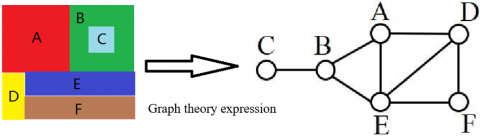
Graph theory is the most popular method to describe the attributes of simple and composite objects, as well as the relationship between them [21]. In the analysis of remote sensing images, graph theory is often adopted to analyze the correlation and structure between image units. Figure 5 expresses the spatial distribution of geographical
In order to realize the description of attributes and relationships from simple objects to composite objects, the most used method is graph theory. In the field of remote sensing image analysis, graph theory is also used to analyze the relationship and structure between image units. Figure 5 shows an example of graph theory expression of spatial distribution of geographic objects.
Figure 5. Graph theory expression of spatial distribution of geographic objects
In this paper, the relational attribute neighborhood graph (RANG) is proposed to represent the hierarchical structure of simple objects and composite objects. The RANG was defined as a seven tuple $(V, E, V P, E P, S, A, P)$, where V is the set of simple objects, E is the set of spatial relationships between simple objects, VP is the set of attributes of simple objects, EP is the set of attributes related to E, S is the set of labels of composite objects, A is the set of attributes of composite objects, and P is the probability that a composite object is assigned with a label in S, which meaures the accuracy of the label assignment. Below is a detailed introduction to each element in the tuple.
Each simple object in V has a unique identity, which can be directly used. The set E can be expressed as:
$E=\left\{r_{1}, r_{2}, \ldots, r_{i}\right\}$
where, $r_{i} \in E$ is a spatial relationship. The spatial relationship between two objects is equivalent to an edge between them:
$r_{i}=\left\{\left\{v_{1}, v_{2}\right\}, \ldots\left\{v_{i}, v_{j}\right\}\right\}$
where, vi and vj is a pair of objects with the spatial relationship of ri.
The set VP records the nonspatial features of each node, including both morphological features and semantic attributes. The morphological features cover plane attributes (e.g. area, perimeter, length and width), shape attributes (e.g. compactness, ellipticity, rectangularity, fractal dimension, and angle) and 3D surface and volume attributes (e.g. volume, height, and surface area). The semantic attributes stand for the subject semantics between simple objects and the most representative semantic attributes of composite objects.
In this paper, two centrality measures, degree centrality and betweenness centrality, are adopted to extract semantic attributes. The centrality measures describe the dominant simple object, i.e. the simple object with the greatest impact on the formation of the corresponding composite object. The degree centrality is defined as the number of nodes directly connected to the current node, that is, the node degree. The degree centrality of node v can be defined as:
$C_{D}(v)=k(v)$
where, k is the node degree. The degree centrality of the network can be defined as:
$C_{D}=\frac{\sum_{i}^{n}\left|C_{D}\left(v^{*}\right)-C_{D}\left(v_{i}\right)\right|}{(n-1)(n-2)}$
where, v* is the node with the highest centrality.
The betweenness centrality, a.k.a. the intermediate centrality, a measure of centrality in a graph based on shortest paths. It mainly evaluates the impact of a simple object on the information flow of the entire composite network. The betweenness centrality of node v can be defined as:
$C_{B}(v)=\sum_{s \neq v \neq t \in V} L_{s t}(v) / L_{s t}$
where, $L_{s t}(v)$ is the number of shortest paths between nodes s and t through node v; $L_{s t}$ is the number of shortest paths between nodes s and t.
Therefore, the VP can be expressed as:
$V P=\left\{m_{1}, m_{2}, \ldots, m_{n}, L_{s}, C_{D}, C_{B}\right\}$
where, $m_{i}$ is the i-th morphological feature; $L_{S}$ is the semantic information on the labels of nodes; $C_{D}$ and $C_{B}$ are degree centrality and betweenness centrality, respectively.
The set EP records the spatial attributes of each edge, such as distance and spatial arrangement. The frequency of each spatial arrangement is also saved in the set to quantify the spatial relationship between simple objects. This attribute of spatial arrangement is also called adjacency-event measurement. Apart from measuring the spatial relationship between simple objects, EP can be coupled with VP to extract more measurement features.
The definition of EP can be established based on the connectivity, an important index of graph structure in graph theory. The connectivity has a positive correlation with the stability of the graph structure. In general, the connectivity level equals the ratio between the number of edges (e) and the number of nodes (v) in the graph:
$\beta=e / v$
Therefore, the set EP can be expressed as:
$E P=\left(\begin{array}{ccc}{p_{11}} & {\cdots} & {p_{1 t}} \\ {\vdots} & {\ddots} & {\vdots} \\ {p_{t 1}} & {\cdots} & {p_{t t}}\end{array}\right)$
where, $p_{i j}$ is the number of adjacent labels i and j of different objects; t is total number of object labels.
The set S contains the semantic labels of composite objects. Each label records the semantic properties of the corresponding object. The label of a composite object can be completed through comprehensive analysis on the morphological attributes, spatial relations and semantics of the lower-level simple objects. The set S can be expressed as:
$S=\left\{s_{1}, s_{2}, \dots, s_{v}\right\}$
where, $S_{i} \in S$ is the i-th semantic label.
The set A stores the morphological attributes of composite objects. It can be expressed as:
$A=\left\{a_{1}, a_{2}, \dots, a_{n}\right\}$
where, $a_{i} \in A$ is the i-th morphological attribute.
The element P represents the probability that a composite object is assigned with a label in S:
$P=\left\{p_{1}, p_{2}, \dots, p_{v}\right\}$
where, $p_{i} \in P$ is the probability that the composite object is assigned with the i-th semantic label. To ensure the correctness of assignment, a composite object is generally given the semantic label with the maximum probability.
As a conceptual expression, the RANG synthesizes the attribute relationships, spatial relationships, semantic relationships and structural relationships involved in the abstraction of composite objects from simple objects, organizes simple and composite objects in a logical geometry, and records the orderly hierarchical relationships between the two types of objects. The RANG provides a data model about the transition to advanced knowledge system and information mining.
4.2 RANG-based classification of urban land use
In this paper, the land cover elements are regarded as simple objects, while the land use units are considered as composite objects. The RANG was adopted to extract the information about land use.
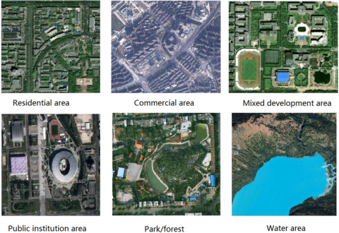
Firstly, the land cover data were classified into six classes: water, trees, grasses/shrubs, bare land, buildings and impermeable ground. The land use data were selected to verify the effectiveness of the RANG-based classification. The data cover six types of land use: residential area, commercial area, mixed development area, public institution area, park/forest and water area. Figure 6 shows the high-definition remote sensing images of the six types of land use.
The RANG-based classification of urban land use was carried out in the following steps. Firstly, the land cover data were objectified, creating the land cover elements (simple objects). Next, the block boundaries were delineated, and the RANG of the relationship between the land cover elements was established for each block was established. From the RANG, the semantic features, spatial relationship features, connectivity features and morphological features were obtained for each block. Taking the blocks as the units of spatial analysis, the random forest algorithm was adopted to evaluate the importance of relevant features, identify the most important features and classify the land use units (composite objects). Finally, the classification results were compared with the actual data on land use.
Figure 6. The high-definition remote sensing images of the six types of land use
Drawing on the relevant literature, 32 feature indices (Table 1) were extracted from the sets VP and EP of the RANG, according to the prior knowledge of the study area.
The four types of features in Table 1 were synthetized, producing a 1D vector containing the 32 feature indices for each block. This vector provides a panorama of the land cover elements in the corresponding block, and can be directly used to identify the type of land use.
As mentioned before, the random forest algorithm, a combinatory algorithm with multiple decision tree-based classifiers, was adopted to classify the land use in the study area. To establish the random forest model, 1,922 blocks were randomly selected as training samples, and the remaining 4,538 blocks were taken as test samples [22].
First, all 32 feature indices were inputted into the random forest training. The error curve of the model was observed through trial and error. The results show that the model has the minimum error with eight split nodes and 500 decision trees. The trained model was adopted to classify the 4,538 blocks in the test set. The overall classification accuracy was 89.11%.
To verify the robustness of our method, different training samples were used to carry out 30 repeated experiments. The producer precision (PA) and user precision (UA) of each type of land use type are shown in Table 2.
Table 1. Feature indices for random forest algorithm
|
Type of features |
Feature indices |
|
Semantic features |
Type of land cover with the highest centrality ($L_1$) |
|
Type of land cover with the highest betweenness centrality ($L_2$) |
|
|
Type of land cover with the second highest centrality ($L_3$) |
|
|
Type of land cover with the second highest betweenness centrality ( $L_4$) |
|
|
Mean centrality of buildings ($L_5$) |
|
|
Spatial features |
Proportion of edges adjacent to water area ($L_6$) |
|
Proportion of edges adjacent to trees ($L_7$) |
|
|
Proportion of edges adjacent to grasses/shrubs ($L_8$) |
|
|
Proportion of edges connected by buildings and trees ($L_9$) |
|
|
Proportion of edges connected by buildings and grasses/shrubs ($L_{10}$) |
|
|
Proportion of buildings adjacent to trees ($L_{11}$) |
|
|
Proportion of buildings adjacent to grasses/shrubs ($L_{12}$) |
|
|
Proportion of buildings surrounded by trees ($L_{13}$) |
|
|
Proportion of buildings surrounded by grasses/shrubs ($L_{14}$) |
|
|
Adjacent diversity of buildings ($L_{15}$) |
|
|
Connectivity features |
Beta index ($L_{16}$) |
|
Morphological features |
Water coverage ratio ($L_{17}$) |
|
Trees coverage ratio (($L_{18}$) |
|
|
Grasses /shrubs coverage ratio ($L_{19}$) |
|
|
Bare land coverage ratio (($L_{20}$) |
|
|
Building coverage ratio ($L_{21}$) |
|
|
Mean compactness of buildings ($L_{22}$) |
|
|
Mean rectangularity of buildings ($L_{23}$) |
|
|
Maximum building area ($L_{24}$) |
|
|
Building average area ($L_{25}$) |
|
|
Number of buildings ($L_{26}$) |
|
|
Building density ($L_{27}$) |
|
|
Block area ($L_{28}$) |
|
|
Block circumference ($L_{30}$) |
|
|
Block compactness ($L_{31}$) |
|
|
Block rectangularity ($L_{32}$) |
Table 2. Statistical results of 30 repeated experiments
|
Precision |
Measurement |
Commercial area |
Mixed development area |
Park/forest |
Public institution area |
Residential area |
Water area |
|
PA |
Mean |
0.781 |
0.703 |
0.858 |
0.585 |
0.964 |
0.872 |
|
Standard deviation |
0.037 |
0.046 |
0.027 |
0.061 |
0.013 |
0.012 |
|
|
UA |
Mean |
0.847 |
0.836 |
0.691 |
0.672 |
0.939 |
0.911 |
|
Standard deviation |
0.028 |
0.041 |
0.019 |
0.045 |
0.011 |
0.012 |
As shown in Table 2, mean accuracy of 30 repeated experiments was 86.2%, with a standard deviation of 2.8%. Among the six types of land use, residential area and water area were recognized and classified at the highest accuracy and stability, while the public institution area saw great fluctuations in the accuracy of recognition and classification.
This paper proposes a novel way to classify urban land use based on graph theory and the GIS. Firstly, the abstraction of composite objects from simple objects, and the hierarchical structure between the objects, were discussed in details. On this basis, each land use unit (composite object) was considered the combination of multiple land cover elements (simple objects). This is in line with our perception of land use in urban areas. Next, a RANG was plotted between land cover elements and four kinds of attributes of these units: semantic features, spatial features, connectivity features and morphological features. In this way, the hierarchical structure of land cover elements and land use units were established. Drawing on the object-based method, the random forest algorithm was introduced to classify the land use in an urban area, and achieved the mean classification accuracy of 86.2%. The research results provide a desirable tool for land use classification, which is of great applicability in the context of rapid urbanization.
[1] Goodchild, M.F. (1992). Geographical data modeling. Computers and Geosciences, 18(4): 401-408. https://doi.org/10.1016/0098-3004(92)90069-4
[2] Tiede, D. (2014). A new geospatial overlay method for the analysis and visualization of spatial change patterns using object-oriented data modeling concepts. Cartography and Geographic Information Science, 41(3): 227-234. https://doi.org/10.1080/15230406.2014.901900
[3] Alesheikh, A.A. (1998). Modeling and managing uncertainty in object-based geospatial information systems, Calgary.
[4] Klien, E. (2007). A rule-based strategy for the semantic annotation of geodata. Transactions in GIS, 11(3): 437-452. https://doi.org/10.1111/j.1467-9671.2007.01054.x
[5] Baja, S., Chapman, D.M., Dragovich, D. (2002). A conceptual model for defining and assessing land management units using a fuzzy modeling approach in GIS environment. Environmental Management, 29(5): 647-661. https://doi.org/10.1007/s00267-001-0053-8
[6] Lü, G., Batty, M., Strobl, J., Lin, H., Zhu, A.X., & Chen, M. (2019). Reflections and speculations on the progress in Geographic Information Systems (GIS): A geographic perspective. International Journal of Geographical Information Science, 33(2): 346-367. https://doi.org/10.1080/13658816.2018.1533136
[7] Wang, C., Xu, M., Wang, X., Zheng, S., & Ma, Z. (2013). Object-oriented change detection approach for high-resolution remote sensing images based on multiscale fusion. Journal of Applied Remote Sensing, 7(1): 073696. https://doi.org/10.1117/1.JRS.7.073696
[8] Pinheiro, P.O., Lin, T.Y., Collobert, R., Dollár, P. (2016). Learning to refine object segments. In European Conference on Computer Vision, pp. 75-91. https://doi.org/10.1007/978-3-319-46448-0_5
[9] Zhang, J., Li, P.J., Wang, J.F. (2014). Urban built-up area extraction from Landsat TM/ETM+ images using spectral information and multivariate texture. Remote Sensing, 6(8): 7339-7359. https://doi.org/10.3390/rs6087339
[10] Gavankar, N.L., Ghosh, S.K. (2018). Automatic building footprint extraction from high-resolution satellite image using mathematical morphology. European Journal of Remote Sensing, 51(1): 182-193. https://doi.org/10.1080/22797254.2017.1416676
[11] Hu, F., Xia, G.S., Hu, J.W., Zhang, L.P. (2015). Transferring deep convolutional neural networks for the scene classification of high-resolution remote sensing imagery. Remote Sensing, 7(11): 14680-14707. https://doi.org/10.3390/rs71114680
[12] Borna, K., Moore, A.B., Sirguey, P. (2016). An intelligent geospatial processing unit for image classification based on geographic vector agents (GVAs). Transactions in GIS, 20(3): 368-381. https://doi.org/10.1111/tgis.12226
[13] Worboys, M. (1998). Imprecision in finite resolution spatial data. GeoInformatica, 2(3): 257-279. https://doi.org/10.1023/A:1009769705164
[14] Mo, L.J., Cao, Y., Hu, Y.M., Liu, M., Xia, D. (2012). Object-oriented classification for satellite remote sensing of wetlands: A case study in southern Hangzhou bay area. Wetland Science, 10(2): 206-213.
[15] Yue, P., Di, L.P., Wei, Y.X., Han, W.G. (2013). Intelligent services for discovery of complex geospatial features from remote sensing imagery. ISPRS Journal of Photogrammetry and Remote Sensing, 83: 151-164. https://doi.org/10.1016/j.isprsjprs.2013.02.015
[16] Barr, S., Barnsley, M. (1997). A region-based, graph-theoretic data model for the inference of second-order thematic information from remotely-sensed images. International Journal of Geographical Information Science, 11(6): 555-576. https://doi.org/10.1080/136588197242194
[17] Belgiu, M., Drăguţ, L. (2016). Random forest in remote sensing: A review of applications and future directions. ISPRS Journal of Photogrammetry and Remote Sensing, 114: 24-31. https://doi.org/10.1016/j.isprsjprs.2016.01.011
[18] Gao, Z.Q., Ning, J.C., Gao, W. (2009). Response of land surface temperature to coastal land use/cover change by remote sensing. Transactions of the Chinese Society of Agricultural Engineering, 25(9): 274-281.
[19] Wang, L.W., Wei, Y.X., Niu, Z. (2008). Spatial and temporal variations of vegetation in Qinghai Province based on satellite data. Journal of Geographical Sciences, 18(1): 73-84. https://doi.org/10.1007/s11442-008-0073-x
[20] Jansen, L.J.M., Di Gregorio, A. (2002). Parametric land cover and land-use classifications as tools for environmental change detection. Agriculture, Ecosystems & Environment, 91(1-3): 89-100. https://doi.org/10.1016/S0167-8809(01)00243-2
[21] Vergniory, M.G., Elcoro, L., Wang, Z.J., Cano, J., Felser, C., Aroyo, M.I., Andrei Bernevig, B., Bradlyn, B. (2017). Graph theory data for topological quantum chemistry. Physical Review E, 96(2): 023310. https://doi.org/10.1103/PhysRevE.96.023310
[22] Chen, W., Xie, X.S., Peng, J.B., Shahabi, H., Hong, H.Y., Bui, D. T., Duan, Z., Li, S.J., Zhu, A.X. (2018). GIS-based landslide susceptibility evaluation using a novel hybrid integration approach of bivariate statistical based random forest method. Catena, 164: 135-149. https://doi.org/10.1016/j.catena.2018.01.012