Bo Guan* | Minghui Liu
OPEN ACCESS
To solve the narrow bandwidth and high error rate of video transmission on the wireless channel, this paper reviews the current video coding standard and improves the original code rate control algorithm. The improvement mainly includes modifying the calculation method for the first quantization parameter QPst and enhancing the effect of the previous group of pictures (GOP) on the QPst of the current GOP. The improved algorithm effectively overcomes the constraint of the channel bandwidth of wireless sensor network (WSN) on the code rate outputted by the video encoder. Considering the cause of the high bit error rate of WSN channel transmission, the inaccuracy of the side matching algorithm (SMA) in processing boundary macroblocks with high difference in pixel luminance was corrected by the boundary matching algorithm (BMA), and the secondary error concealment was introduced to better utilize the completely concealed macroblock information and improve the quality of the reconstructed image. The improved error concealment algorithm was proved more effective than the original algorithm in the quality of image reconstruction through experiments.
wireless sensor network (WSN), rate control, error concealment
The video transmission on the wireless channel faces such problems as narrow bandwidth, great bandwidth volatility and high error rate. This calls for a video compression coding standard, which is suitable for a low bandwidth environment and capable of maximizing the video quality at a given code stream.
The videos processed by the H.264 coding standard support video communication. So far, many improved rate control algorithms have been developed based on this standard. For instance, Andrew Armstrong, [1] proposed a method to optimize the initial QP, in which the QP value is determined through binary search. [2] created an enhanced rate and rate-distortion model, which solves the “chicken or the egg causality dilemma” in H.264 standard using QP estimation and update, and enhances the accuracy by adjusting the number of bits occupied by the header information at a low bit rate. [3] set up a rate-distortion model in ρ domain according to the statistical relationship between the proportion of non-zero values of discrete cosine transform (DCT) coefficients in the coefficient table and the code rate.
In addition, many scholars have proposed error concealment techniques. For example, [4] developed a zero-motion vector method for images with weak motion intensity, which makes up for the data loss at the decoder with the macroblock at the same position in the reference frame. [5] put forward the boundary matching algorithm (BMA) capable of preventing boundary problems like edge breakage and object deformation; By this method, the error is concealed by multiple motion vectors in different regions of the damaged macroblock instead of a single motion of the macroblock.
In light of the above, this paper probes into the video compression technology in the wireless transmission environment, aiming to achieve efficient video encoding and decoding and make the encoded code stream suitable for transmission in wireless sensor network (WSN) channels. Two key problems are tackled in this research: How to handle the compressed video stream at the encoder end to make the bandwidth suitable for wireless transmission without sacrificing video quality; how to decode the error-containing video sequence received at the decoder end to minimize the video quality degradation in wireless transmission.
2.1 Rate-distortion theory
The rate-distortion theory lays the theoretical basis for the quantization process in video processing. The theory mainly tackles the difference between the symbols received by the sink and the signals sent by the source after encoding, error-free transmission and decoding. The difference can be measured by the amount of information, that is, entropy. The rate-distortion function, denoted as the R(D) function, describes the minimum amount of mutual information to be transmitted for a given source, when the average distortion does not exceed a pre-set degree of distortion. For source coding, the function specifies the lower limit of the code stream information rate after the message sent by the source is compression-encoded under the pre-set degree of distortion. The rate-distortion function can be expressed as:
$R(D)=\min I(A ; B)$ (1)
where D is a given mean distortion value.
2.2 Predictive coding
In video compression encoding, the predictive coding can be classified into intra-frame prediction coding and inter-frame prediction coding by the positions of the pixels selected for prediction. In intra-frame prediction, the pixels to be predicted are selected from adjacent positions in the local frame of the elements to be encoded; In inter-frame coding, the elements in temporally adjacent frames are selected for prediction.
Both intra- and inter-frame prediction coding modes are adopted in the H.264 standard. The encoder can recognize the pattern of each macroblock, and determine the suitable coding mode for the current macroblock need. The inter-frame prediction coding will be changed by the encoder into the intra-frame mode, when the image quality is degraded due to error accumulation or the motion threshold is not reached.
2.3 Quantification
The compression by block-based video encoder is essentially a quantization of the transform coefficients. Here, quantization refers to the process of converting continuous input signals into a finite number of output signals. During the quantization, the DCT-transformed coefficients are mapped to reduced values, thereby reducing the number of bits of block coding. The number of output bits of block-based encoder can be adjusted through the control of the quantizer. This strategy is adopted in this paper to control the output rate of the encoder.
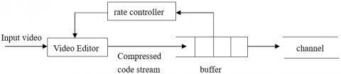
As its name suggests, the rate control problem aims to control the bit rate outputted by the encoder through adjustment of coding parameters (e.g. frame rate, motion detection threshold and QP) according to the actual state information (e.g. code rate, delay and buffer) and the rate-distortion theory. The philosophy of rate control is presented in Figure 1. During the rate control, the rate controller controls the output code stream of the video encoder, while the buffer smooths the output bit rate. The code rate at the input of the buffer is varying, while that at the output of the buffer depends on the rate control algorithm.
Figure 1. Philosophy of rate control
The rate control in this paper attempts to ensure the match between the video stream and the available network bandwidth, thereby mitigating network congestion and smoothing the output stream of the encoder.
3.1 H.264 rate control algorithm
The H.264 rate control algorithm was developed on the basis of the basic unit, the fluid motion traffic model, and the mean absolute difference (MAD) linear prediction model. If a basic unit is divided into sub-units in the size of one frame, then the rate control only involves two layers, namely, the group of pictures (GOP) layer and the frame layer. The GOP layer rate control algorithm includes two steps: determining the target number of bits and initializing the QP.
Step 1. Determining the number of bits to be coded for the GOP layer
Before the encoding of the i-th GOP, the total number of bits to be allocated to the GOP can be calculated as:
$T_{r}\left(n_{i, 0}\right)=\frac{u\left(n_{i, 1}\right)}{F_{r}} \times N_{g o p}-B_{c}\left(n_{i-1, N_{g o p}}\right)$ (2)
where $N_{g o p}$ is the number of frames contained in the GOP. Since the channel has a time-varying bandwidth, Tr is continuously updated in units of frames according to the following equation:
$T_{r}\left(n_{i, j}\right)=T_{r}\left(n_{i, j-1}\right)+\frac{u\left(n_{i, j}\right)-u\left(n_{i, j-1}\right)}{F_{r}}\left(N_{g o p}-j\right)-b\left(n_{i, j-1}\right)$ (3)
If the code rate is fixed, then $u\left(n_{i, j}\right)=u\left(n_{i, j-1}\right)$ can be simplified to equation (4), that is, equation (2) specifies the number of bits to be allocated to a GOP under a fixed code rate.
$T_{r}\left(n_{i, j}\right)=T_{r}\left(n_{i, j-1}\right)-b\left(n_{i, j-1}\right)$ (4)
Step 2. Initializing the QP
The initial QP, denoted as QP0, is estimated based on the available channel bandwidth and the GOP length. QP0 is the QP used to encode the I frame and the first P frame of the first GOP in the frame sequence. In general, the QP0 value should be negatively correlated with the channel bandwidth, and reduced by a unit every time the GOP length increases by 30. The value of QP0 can be calculated as:
$Q P_{0}=\left\{\begin{array}{ll}{40} & {b p p \leq l_{1}} \\ {30} & {l_{1}<b p p<l_{2}} \\ {20} & {l_{2}<b p p \leq l_{3}} \\ {10} & {b p p>l_{3}}\end{array}\right.$ (5)
$b p p=u\left(n_{0,0}\right) / F_{r} N_{p i x e l}$ (6)
where bpp is the number of bits occupied by each pixel; $N_{p i x e l}$ is the total number of pixels per each frame of image.
Except for the first GOP, the first QP QPst in other GOPs can be calculated as:
$Q P_{s t}=\frac{\operatorname{sum}_{P Q P}}{N_{p}}-\frac{8 \times \operatorname{Tr}\left(n_{i-1, N_{g o p}}\right)}{\operatorname{Tr}\left(n_{i, 0}\right)}-\min \left\{2, \frac{N_{g o p}}{15}\right\}$ (7)
where Np is the number of all P frames in the previous GOP; $Sum_{pep}$ is the sum of the QPs of all P frames in the previous GOP.
3.2 Improvement of rate control algorithm
In the GOP layer rate control of the H.264 standard, the QP of the I frame and the first P frame of the first GOP in the frame sequence, denoted as QP0, is configured in advance, while the initial QPs of the other GOPs, denoted as QPst, are calculated by equation (7). However, it has been proved through repeated experiments that the H.264 rate control algorithm may lead to a huge difference in peak signal-to-noise ratio (PSNR) at different initial PQs of the same video sequence, especially when the initial QPs are extremely small.
The PSNR, an objective evaluation indicator of video quality, can be calculated as:
$P S N R=10 \times \log \left(\frac{255^{2}}{M S E}\right)$ (8)
$M S E=\frac{1}{M \times N} \sum_{i=0}^{M-1} \sum_{j=0}^{N-1}(x(i, j)-y(i, j))^{2}$ (9)
where M is the width of the image; N is the height of the image; x(i,j) is the luminance or chrominance at (i,j) of the original image; y(i,j) is the luminance or chrominance at (i,j) after decoding. The unit of PSNR is dB.
$P S N R_{a v g}=\left(4 \times P S N R_{Y}+P S N R_{U}+P S N R_{V}\right) / 6$ (10)
where the variables PSNRY, PSNRU and PSNRV are the PSNR values of components Y, U and V obtained by the Joint Model (JM).
JM8.6 was adopted for our experimental platform. The parameter settings of the encoder in the JM test model are stored in the file encoder.cfg, and the corresponding parameter settings of the decoder are stored in the file decoder.cfg. In the rate control experiment, the encoder functions can be controlled by modifying the corresponding parameters in the file encoder.cfg. Some of the parameters in our experiment were configured as follows:
(1) FramesToBeEncoded=100;
(2) Framerate=30;
(3) Number Frames=0;
(4) Frame Skip=0;
(5) Search Range=16;
(6) InitialQP=15;
(7) RateControlEnable=1。
The first 100 frames in news_qcif and those in grandma_qcif were taken as the standard test sequences used in our experiment, with target bit rates of 128kbps and 64 kbps, respectively. The experimental results on the two sequences are listed in Table 1 below.
Table 1. Experimental results on sequences news_qcif and grandma_qcif
|
InitialQP |
news_qcif Actual code rate (kbps) |
news_qcif Actual PSNRavg (dB) |
grandma_qcif Actual code rate (kbps) |
grandma_qcif Actual PSNRavg (dB) |
|
15 |
154.98 |
39.39 |
118.76 |
40.21 |
|
16 |
142.26 |
38.89 |
107.28 |
39.77 |
|
17 |
131.33 |
38.41 |
97.99 |
39.27 |
|
18 |
129.29 |
38.45 |
88.57 |
38.80 |
|
19 |
129.20 |
38.58 |
80.94 |
38.31 |
|
20 |
128.94 |
38.66 |
73.36 |
37.84 |
|
21 |
129.01 |
38.59 |
66.42 |
37.38 |
|
22 |
129.37 |
38.65 |
64.13 |
37.28 |
|
23 |
129.12 |
38.65 |
64.32 |
37.47 |
|
24 |
129.59 |
38.55 |
64.44 |
37.54 |
|
25 |
129.47 |
38.58 |
64.39 |
37.42 |
|
26 |
128.93 |
38.38 |
64.56 |
37.43 |
|
27 |
128.94 |
38.31 |
64.50 |
37.31 |
|
28 |
129.05 |
38.20 |
64.60 |
37.16 |
|
29 |
129.08 |
38.26 |
64.63 |
37.07 |
|
30 |
129.32 |
38.23 |
64.44 |
37.06 |
As shown in Table 1, when the QP was small (e.g. InitialQP=15), the actual code rate deviated from the target code rate by more than 21 %; moreover, the actual code rate and PSNR generated by the encoder fluctuated greatly with the InitialQPs. This is attributable to the underestimation of the impact of GOP code rate on QPst when the GOP layer rate control algorithm computed the initial QP QPst . As a result, the initial QP of the I frame and the first P frame was not calculated accurately, leading to inaccurate bit number allocation to the GOP, which in turn affected the quality and code rate of the video.
The above problem was solved through the improvement below.
Step 1. Calculation of QP0
When the encoder starts to process a video sequence, the first frame of the first GOP is treated as an I frame. Because it is the first frame, there is no reference information. Hence, the encoder uses the inherent QP. The initial QP QP0 is still calculated by equation (5), where l1, l2 and l3 are 0.1, 0.3 and 0.6, respectively.
Step 2. Calculation of QPst
According to the rate-distortion (R-D) model, the number of bits generated after the encoding of the i-1-th GOP, denoted as bi-1, can be expressed as:
$b_{i-1}=M A D \times\left(\frac{a_{1}}{Q_{ {avestep}}}+\frac{a_{2}}{Q_{{avestep}}^{2}}\right)$ (11)
where Qavestep is the quantization step length corresponding to the mean QP of the P frames in the i-1-th GOP.
Let Qststep be the quantization step length of QPst . Then, the number of bits generated after the encoding of the i-th GOP, denoted as bi, can be expressed as:
$b_{i}=M A D \times\left(\frac{a_{1}}{Q_{s t s t e p}}+\frac{a_{2}}{Q_{s t s t e p}^{2}}\right)$ (12)
$\alpha=\frac{b_{i-1}}{b_{i}}, \beta=\frac{a_{2}}{{ Q_{avestep} } \times a_{1}}$ and $\gamma=\frac{Q_{ {ststep}}}{ {Q_{avestep}}}$. Dividing equation (11) by equation (12), we have:
$\gamma^{2}-\frac{\alpha}{1+\beta} \times \gamma-\frac{\alpha \times \beta}{1+\beta}=0$ (13)
Solving equation (13), we have:
$Q_{ {ststep}}=\frac{2}{\sqrt{1+\frac{4 \times(1+\beta)}{\alpha}}} \times Q_{ {avestep}}$ (14)
The QP QPst can be obtained according to equation (14).
Let QPave be the QP corresponding to Qavestep. Then, QPst must be subjected to the following constraint:
$Q P_{s t}=\min \left(\max \left(Q P_{a v e}-2, Q P_{s t}\right), Q P_{a v e}+2\right)$ (15)
where α is calculated during the determination of the number of bits needed for each GOP; β is initialized as 1 and updated constantly during the encoding process.
3.3 Experiment and analysis
The improved algorithm was applied in another experiment on JM8.6 under the same experimental conditions as the previous experiment. The experiment targets the standard test sequences of news_qcif and grandma_qcif, with target bit rates of 128kbps and 64 kbps, respectively. The experimental results of the improved algorithm are recorded in Table 2 below.
Table 2. Experimental results of the improved algorithm
|
InitialQP |
news_qcif Actual code rate (kbps) |
news_qcif Actual PSNRavg (dB) |
grandma_qcif Actual code rate (kbps) |
grandma_qcif Actual PSNRavg (dB) |
|
15 |
128.77 |
38.65 |
64.19 |
36.89 |
|
16 |
129.30 |
38.86 |
64.40 |
37.14 |
|
17 |
129.55 |
38.95 |
64.37 |
37.95 |
|
18 |
128.78 |
39.07 |
64.45 |
38.04 |
|
19 |
129.10 |
39.15 |
64.31 |
37.85 |
|
20 |
129.11 |
38.99 |
64.35 |
38.69 |
|
21 |
128.82 |
38.98 |
64.41 |
38.63 |
|
22 |
128.56 |
38.90 |
64.25 |
38.53 |
|
23 |
128.97 |
38.87 |
64.35 |
38.34 |
|
24 |
128.82 |
38.75 |
64.36 |
38.18 |
|
25 |
128.53 |
38.52 |
64.42 |
37.96 |
|
26 |
129.05 |
38.38 |
64.36 |
37.70 |
|
27 |
128.69 |
38.29 |
64.44 |
37.44 |
|
28 |
128.86 |
38.23 |
64.39 |
37.42 |
|
29 |
128.76 |
38.34 |
64.38 |
37.38 |
|
30 |
128.97 |
38.32 |
64.42 |
37.32 |
As mentioned before (Table 1), the initial QP of the original rate control algorithm greatly affected the code rate outputted by the video encoder and the PSNR, an indicator of video quality. By contrast, the improved algorithm performed well in the control of the code rate and the PSNR (Table 2). Compared with the original algorithm, the improved algorithm solved the variation in code rate with initial QP values, outputted a close-to-target code rate, and enhanced the controllability of the code rate. In addition, the improved algorithm realized a smaller error and a higher PSNR than the original algorithm.
4.1 Improvement of the BMA
The side matching algorithm (SMA) is a popular way to conceal the error of missing macroblocks in the P frame, thanks to its good performance in treating homogenous pixels. However, the SMA may suffer from a huge error if applied to macroblocks with a significant difference in pixel luminance. This defect can be overcome by the BMA, which offsets the matching error between the boundary pixels of the macroblocks adjacent to the target macroblock and those of the macroblocks adjacent to the missing macroblock.
Here, the SMA is improved to conceal the erroneous P frame in two steps. Firstly, all erroneous macroblocks in the predictive frame, which contains such macroblocks, are concealed to roughly improve the image quality, laying the basis for error correction in the second step. Secondly, the motion vectors of the erroneous macroblocks treated in the first step are assigned proper weights and subjected to error correction, aiming to achieve accurate error processing.
Step 1: Primary concealment
A motion vector is roughly estimated for each missing macroblock, and a motion compensation block is found in the corresponding reference frame to replace the missing macroblock. Let MBcurrent be the current erroneous macroblock to receive concealment, MBtop be the adjacent macroblock directly above the current erroneous macroblock, MBdown be the adjacent macroblock directly below the current erroneous macroblock, and MBbefore be the macroblock in the previous frame at the same position as the current erroneous macroblock. Then, the motion vector of MBcurrent for primary concealment is one of the three motion vectors corresponding to MBtop, MBdown and MBbefore. Considering the difference of macroblock size in different frames (the macroblocks in each frame are either all 8x8 or all 4x4), the mean motion vector of all sub-blocks in a macroblock is taken as the motion vector of the entire macroblock. The motion vector of MBcurrent for primary concealment can be calculated as:
1. The motion vector of MBbefore should be adopted as that of MBcurrent, provided that MBbefore has no damage, adopts inter-frame coding, and its motion vector moves within 8 pixels in the horizontal and vertical directions. In this case, the images in the frame sequence move slowly, and MBcurrent basically maintains the motion trend of MBbefore .
2. The motion vector of MBtop should be adopted as the primary concealment motion vector, provided that MBtop has no damage, adopts inter-frame coding and lies not on boundaries. In this case, the images in the frame sequence move violently and the motion of MBcurrent is not very consistent with that of MBbefore. Thus, the motion correlation between adjacent macroblocks in the current frame should be considered.
3. The motion vector of MBdown should be adopted as the primary concealment motion vector, provided that MBdown has no damage, adopts inter-frame coding and lies not on boundaries.
4. Otherwise, the zero-motion vector should be taken as the motion vector for primary concealment.
Step 2. Weighted boundary matching
The motion vector of the macroblock that has received primary error concealment is adopted to maximize the image quality. The boundary matching is performed for the entire missing macroblock using multiple weights according to equation (16). The motion vector with the minimal V value should be selected from the set of candidate motion vectors C to serve as the motion vector for secondary error concealment.
$V(x, y)=\underset{v(x, y) \in C}{\operatorname{argmin}}\left(W_{U} B M E_{U}+W_{D} B M E_{D}+W_{L} B M E_{L}+{W_{R} B M E_{R} )}\right)$ (16)
where WU, WD, WL and WR are the weights of the matching errors with the upper, lower, left and right boundaries of the erroneous macroblock, respectively. The complete macroblock, the primarily concealed macroblock, and the completely concealed macroblock have different weights, which are respectively 1, 0.125 and 0.25.
In this step, the motion vectors of the correct macroblocks adjacent to the erroneous macroblock, that of the macroblock at the same position as the erroneous macroblock in the previous frame, and those of the primarily concealed and completely concealed macroblocks adjacent to the erroneous macroblock are all taken as candidate motion vectors for secondary error concealment algorithm. In this way, the set of candidate motion vectors is enriched and the reconstruction quality of the image is improved.
4.2 Experiment and analysis
The JM8.6 was adopted for our experiment. The packet loss rate of the bit stream generated by video encoding was set to 5%. The parameters in the file encoder.cfg were configured as follows:
(1) Input File="football_qcif.yuv";
(2) FramesToBeEncoded=30;
(3) FrameRate=30;
(4) OutFileMode=1;
(5) Slice Mode=1;
(6) num_slice_groups_minus1=1.
The files formed after compression and encoding were processed randomly at different packet loss rates by rtp_loss. The processed files were then decoded by the decoder, to present the PSNR and subjective quality of the reconstructed image.
Table 3 compares the decoding PSNRavgs of the proposed improved algorithm with the SMA on different standard video sequences at different packet loss rates. It can be seen that the proposed improved algorithm outperformed the original SMA in the quality of the reconstructed video, when the video sequence (e.g. football_qcif) moved relatively violently (i.e. the sum of the mean motion vectors for the horizontal and vertical motions of video images is greater than 8 pixels). Moreover, the proposed algorithm also prevented the degradation of the reconstructed video for the video sequence moving smoothly (e.g. news_qcif).
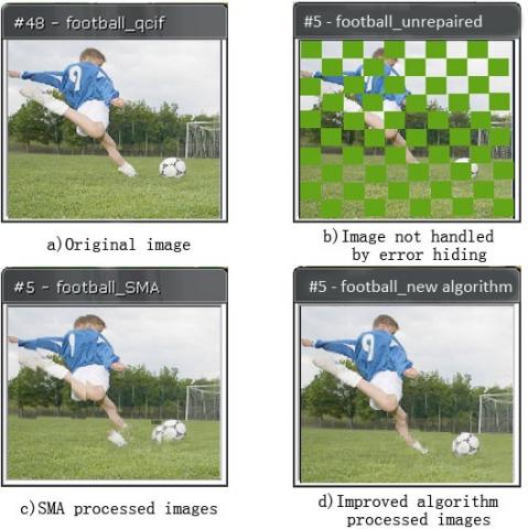
Figure 2 shows the subjective quality of the video images reconstructed from a video stream encoded in chessboard mode by the SMA and the improved algorithm, respectively. It can be seen that the football_qcif sequence processed by the SMA, which is only suitable for video sequences with relatively smooth motion, had a high error in boundary matching, leading to a poor video quality. This is because the sequence has a relatively strong motion. By contrast, the proposed improved algorithm reconstructed high quality video images whether the video sequence moved smoothly or violently.
Table 3. Objective comparison of error concealment effects
|
Sequence of Test Use |
algorithm |
1% packet loss rates PSNRavg (dB) |
5% packet loss rates PSNRavg (dB) |
8% packet loss rates PSNRavg (dB) |
10% packet loss rates PSNRavg (dB) |
|
football_qcif |
SMA |
27.56 |
24.75 |
23.47 |
23.00 |
|
Improved Algorithm |
28.42 |
25.67 |
24.26 |
23.60 |
|
|
mobile_qcif |
SMA |
29.34 |
27.23 |
26.24 |
25.47 |
|
Improved Algorithm |
30.11 |
28.16 |
27.34 |
26.48 |
|
|
news_qcif |
SMA |
38.15 |
36.05 |
35.72 |
35.67 |
|
Improved Algorithm |
38.15 |
36.05 |
35.72 |
35.67 |
Figure 2. Error concealment effect of football_qcif sequence
Through in-depth analysis, the rate control technology in the H.264 standard was found to be unsuitable for the code rate features required for WSN channel transmission. Therefore, the original rate control algorithm was improved to enhance the stability and controllability of the code rate. The improvement mainly includes modifying the calculation method for QPst and enhancing the effect of the previous GOP on the QPst of the current GOP. Considering the cause of the high bit error rate of WSN channel transmission, the inaccuracy of the SMA was corrected by the BMA, and the secondary error concealment was introduced to overcome the shortcoming of the BMA, aiming to better utilize the completely concealed macroblock information and improve the quality of the reconstructed image. The improved algorithm was proved effective through experiments.
This paper is the relevant research result of the Planning Project of the Department of Education "13th Five-Year Plan" Humanities and Social Sciences in Jilin Province in 2018, (Grant No. JJKH20180392SK), and the Planning Project of the Department of Education “13th Five-Year Plan” for Education Science in Jilin Province in 2018(Grant No. GH180074).
[1] Armstrong, A., Beesley, S., Grecos. C. (2006). Selection of initial quantisation parameter for rate controlled. H.264 Video Coding Research in Microelectronics and Electronics, 13(6): 249-252. http://doi.org/10.1109/RME.2006.1689943
[2] Kwon, D.K., Shen, M.Y. (2007). Rate control for h.264 video with enhanced rate and distortion models. IEEE Trans. on Circuits Systems. for Video Techno, 4(7): 517-529. http://doi.org/10.1109/TCSVT.2007.894053
[3] He, Z. (2001). Domainrate-Distortion analysis and rate control for visual coding and communications. Dissertation of University of California Santa Barbara.
[4] Aign, S. (1995). Error concealment enhancement by using the reliability outputs of a SOVA in MPEG-2 video decoder. URSI Int. Symp. Signal Systems and Electronics, pp. 59-62. http://doi.org/10.1109/ISSSE.1995.497934
[5] Chen, T., Zhang, X., Shi, Y.Q. (2005). Error concealment using refined boundary matching algorithm. Information Technology Research and Education, 27(1): 55-59. http://doi.org/10.1109/ITRE.2003.1270571
[6] Zhang, J.L., Wu, C.K., Gao, X.B. (2007). A video error hide algorithm based on double domain Lagrangian interpolation. Electronic Journal, 10(3): 653-658. http://doi.org/10.1109/IIHMSP.2011.93
[7] Shen, L.S., Zhuo, L., Tian, D. (2009). Video coding and low rate transmission. Electronic Industry Press, 12(5): 2-13.
[8] Sun, L.M. (2009). Wireless sensor network. Tsinghua University Press. 2009, 9(5):110-112.
[9] Wang, Y., Zhu, Q.F. (2008). Error control and concealment for video communication. Proceedings of the IEEE. 3(6): 974-977. http://doi.org/10.1109/5.664283
[10] Kim, D., Yang, S., Jeong, J. (2005). A New temporal error concealment method for h.264 using adaptive block sizes. IEEE International Conference on, 38(4): 11-12. http://doi.org/10.1109/ICIP.2005.1530545
[11] Chen, T. (2003). Error concealment using refined boundary matching algorithm. Information Technology, 2(1): 55-59. http://doi.org/10.1109/ITRE.2003.1270571
[12] Yan, B. (2004). A novel motion vector recovery algorithm for error concealment in video transmission. Consumer Communications and Networking Conference, 4(7): 621-623. http://doi.org/10.1109/CCNC.2004.1286934
[13] Park, J., Chul, P.D. (2005). Recovery of image blocks using the method of alternating projectiongs. IEEE Trans. on Image Processing, 13(5): 461-467. http://doi.org/10.1109/TIP.2004.842354
[14] Park, J., Chul, P.D. (2005). Content-based adaptive Spatio-temporal methods for MPEG repair. IEEE Transactions on Image Processing, 5(6): 1066-1077. http://doi.org/10.1109/TIP.2003.822615
[15] Zhang, J., Arnold, J.F., Frater, M.R. (2005). A Cell-loss concealment technique for MPEG-2 coded video. IEEE Transactions on Circuits and Systems for Video Technology, 28(6): 659-665. http://doi.org/10.1109/76.845011
[16] Zhang, J., Zhang, C.T. (2005). Control technology of bitrate in video transmission. Journal of Circuits and Systems, 8(10): 106-110. http://doi.org/10.3969/j.issn.1007-0249.2005.03.023