Biyao Zhang | Kaisong Zhang* | Luo Zhong | Xuanya Zhang
OPEN ACCESS
This paper aims to develop a clustering method that need not predefine the number of clusters or incur a high computing cost. For this purpose, Dirichlet Process Mixture Model (DPMM) which based on nonparametric Bayesian method was introduced. Three datasets, from simple to complex, were selected for experiment. The results of the first two datasets showed that the DPMM is highly flexible and reliable, because it did not need to know the number of clusters in advance and had robustness for different rational parameters. However, the DPMM failed to achieve desirable results in the third dataset. To overcome the limitation of one-time DPMM clustering on complex datasets, the notion of hierarchical clustering was adopted to form the hierarchical DPMM algorithm, which outputted better clustering results than DPMM. In this paper, the rules of selecting parameters and the algorithm of hierarchical DPMM are provided for the effective using of DPMM.
clustering, nonparametric Bayesian, DPMM, hierarchical DPMM
Clustering is an important unsupervised method of data analyzing. The classic clustering algorithms fall into K-means algorithms [1, 2], finite mixture models and density-based methods. The first two categories require the estimation of the number of clusters in the dataset. One of the typical density-based methods is clustering by fast search and find of density peaks (CFDP) [3], which is good at locating the center point of big clusters. However, the location performance is realized at the cost of heavy computing resources. Several attempts [4, 5] have been made to reduce its computing cost and enhance its efficiency. Against this backdrop, it is necessary to develop a clustering method that need not predefine the number of clusters or incur a high computing cost.
The Dirichlet process mixture model (DPMM) [6-10] offers a good basis to design such a clustering method. DPMM is an infinite mixture model which bases on probability distribution and does not have a certain form. The realization of DPMM requires the method of nonparametric Bayesian. To be specific, it relies on Bayesian analysis to figure out the conjugate equation of posterior, and then through sampling, nonparametric means, to obtain the clustering result.
Much research has been done to modify and improve the DPMM. For instance, Reference [11] solves the maximum a posteriori probability (MAP) problem for the DPMM. Reference [12] improves the run-time efficiency of parallel Gibbs sampler of the DPMM. Reference [13] enhances the prediction performance of the DPMM by enriched Dirichlet process. Reference [14] develops a new R package for the DPMM, named PReMiuM. References [15-18] extend the application scope of the DPMM to many new areas.
This paper aims to optimize the applicability of the DPMM for clustering operation. Firstly, the concepts and equations of the DPMM were introduced in details. Then, the effects of parameter estimation rules on result accuracy were investigated. Finally, a hierarchical DPMM algorithm was developed to solve the problems that cannot be handled simply through parameter adjustment.
Clustering can be realized by the model based on probability distribution. It is assumed that the samples are from several different distributions, and each distribution represents a cluster. For the reason of building an infinite mixture model, DPMM adds a new layer of “distribution” onto these different distributions, forming a “distribution of distributions”. The additive “distribution” is the Dirichlet process (DP). The DPMM can be expressed as [19]:
$G \sim D P(\alpha, H)$
$\boldsymbol{\theta}_{i} \sim G$
$\boldsymbol{x}_{i} \sim F\left(\boldsymbol{\theta}_{i}\right)$
Because DP cannot be directly applied to data analysis, the above model can be written as:
$\boldsymbol{\pi} \sim G E M(\alpha)$
$\boldsymbol{Z}_{i} \sim \boldsymbol{\pi}$
$\boldsymbol{\theta}_{k} \sim H(\lambda)$
$\boldsymbol{x}_{i} \sim F\left(\boldsymbol{\theta}_{z_{i}}\right)$
where $\boldsymbol{\pi} \sim G E M(\alpha)$ represents:
$\beta_{k} \sim {Beta}(1, \alpha)$
$\pi_{k}=\beta_{k} \prod_{l=1}^{k-1}\left(1-\beta_{l}\right)=\beta_{k}\left(1-\sum_{l=1}^{k-1} \pi_{l}\right)$
The model has some important equations form [19]:
$p\left(z_{i}=k | z_{-i}, x, \alpha, \lambda\right)\propto p\left(z_{i}=k | z_{-i}, \alpha\right) p\left(x_{i} | x_{-i}, z_{i}=k, z_{-i}, \lambda\right)$ (1)
This equation was obtained by Bayesian Analysis. The left side is posterior, and the right side is the conjugate equation of it. For the first item from the right side of (1):
$p\left(z_{i}=k | \mathbf{z}_{-i}, \alpha\right)=\frac{p\left(\mathbf{z}_{1 : N} | \alpha\right)}{p\left(\mathbf{z}_{-i} | \alpha\right)}=\frac{N_{k,-i}+\frac{\alpha}{K}}{N+\alpha-1}$
because
$\lim _{K \rightarrow \infty} \frac{N_{k,-i}+\frac{\alpha}{K}}{N+\alpha-1}=\frac{N_{k-i}}{N+\alpha-1}$
and
$1-\sum_{k=1}^{K} \frac{N_{k,-i}}{N+\alpha-1}=\frac{\alpha}{N+\alpha-1}$
$p\left(z_{i}=k | \mathbf{z}_{-i}, \alpha\right)=\left\{\begin{array}{ll}{\frac{N_{k-i}}{\alpha+N-1}} & {\text { Existing cluster }} \\ {\frac{\alpha}{\alpha+N-1}} & {\text { New cluster }}\end{array}\right.$ (1.1)
And for the second item from the right side of (1):
$p\left(\boldsymbol{x}_{i} | \boldsymbol{x}_{-i}, z_{i}=k, \boldsymbol{z}_{-i}, \lambda\right)=\left\{\begin{array}{ll}{p\left(\boldsymbol{x}_{i} | D_{k,-i}\right)} & {\text { Existing cluster }} \\ {p\left(\boldsymbol{x}_{i} | \lambda\right)} & {\text { New cluster }}\end{array}\right.$ (1.2)
Then, combining (1.1) and (1.2) the function can be written as:
$p\left(z_{i}=k | \mathbf{z}_{-i}, \boldsymbol{x}, \alpha, \lambda\right) \propto\left\{\begin{array}{ll}{\frac{N_{k-i}}{\alpha+N-1} p\left(\boldsymbol{x}_{i} | D_{k,-i}\right)} & {\text { Existing cluster }} \\ {\frac{\alpha}{\alpha+N-1} p\left(\boldsymbol{x}_{i} | \lambda\right)} & {\text { New cluster }}\end{array}\right.$ (2)
where, $D_{k,-i}=\left\{x_{j} : z_{i}=k, j \neq i\right\}, N_{k,-i}$ is the number of samples in $D_{k,-i}$.
After these calculations, because the model has no specific form of distributions, the clustering result need to be obtained by nonparametric means, Gibbs sampling, which can be referred from Reference [20].
For better understanding, (2) can be transformed into:
$\left\{\begin{array}{ll}{p\left(\boldsymbol{x}_{i} \in c_{k}\right)=\frac{N_{k-i}}{\alpha+N-1} p\left(\boldsymbol{x}_{i} | D_{k,-i}\right)} & {\boldsymbol{x}_{i} \text { belongs to existing cluster } k} \\ {p\left(\boldsymbol{x}_{i} \in c_{n e w}\right)=\frac{\alpha}{\alpha+N-1} p\left(\boldsymbol{x}_{i} | \lambda\right)} & {\boldsymbol{x}_{i} \text { belongs to new cluster }}\end{array}\right.$ (3)
where $\boldsymbol{x}_{i}$ means sample i; ck Means cluster k; $D_{k,-i}=\left\{x_{j} : z_{i}=k, j \neq i\right\} ; N_{k,-i}$ is the number of samples in cluster ck Without $\boldsymbol{x}_{i}$; $\lambda$ is the parameter of base distribution H.
The process of Gibbs sampling is shown below:
Algorithm 1. Gibbs sampling for DPMM
Input: raw dataset
Begin
Normalize and shuffle the raw dataset to get a new set.
Initialize n samples as n different clusters.
For each $\boldsymbol{x}_{i}$ In the new set do:
Remove $\boldsymbol{x}_{i}$ From its current cluster.
For each ck Do:
Compute $p\left(\boldsymbol{x}_{i} \in c_{k}\right)$
End
Compute $p\left(\boldsymbol{x}_{i} \in c_{n e w}\right)$
Find the maximum p.
If $p_{\max }=p\left(\boldsymbol{x}_{i} \in c_{k}\right)$
Assign $\boldsymbol{x}_{i}$ To cluster k.
Else $p_{\max }=p\left(\boldsymbol{x}_{i} \in c_{n e w}\right)$
Assign $\boldsymbol{x}_{i}$ To a new cluster.
End
End
End
Output: the set of data marked by clusters’ number
In this section, three datasets were cited to demonstrate the clustering by the DPMM. The experiment was carried out on MATLAB R2018a (Win 64) in a computer running on Windows 10 (64bit) with Intel® Core™ i7-7700HQ Processor and 32GB RAM.
3.1 Testing of simulated data
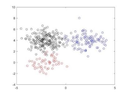
The sample dataset was generated from three 2D-Gaussian distributions: Cluster 1 has 200 samples from $N([-2\,4], I)$, Cluster 2 has 100 samples from $N([2\,4], I)$ and Cluster 3 has 50 samples form $N([-2\,0], I)$. The original point diagram and histogram are shown in Figure 1 below.
Figure 1. Samples of three 2D-Gaussian distributions
In the left part of Figure 1, each cluster is marked in a different color. The Gaussian distribution was taken as the base distribution of the DPMM. Some settings are presented below:
$H(\lambda)=N(0, I)$
$\lambda=\{0, I\}$
$p\left(x_{i} | D_{k,-i}\right)=p\left(x_{i}, | x_{k,-i}, \lambda\right)=\frac{p\left(x_{i}, x_{k,-i} | \lambda\right)}{p\left(x_{k,-i} | \lambda\right)}$
$=\int p\left(x_{i} | \boldsymbol{\theta}_{k}\right) H\left(\boldsymbol{\theta}_{k} | \lambda\right) d \boldsymbol{\theta}_{k}=N\left(\boldsymbol{x}_{i} | \boldsymbol{\theta}_{k}\right)$
$p\left(\boldsymbol{x}_{i} | \lambda\right)=\int p\left(\boldsymbol{x}_{i} | \boldsymbol{\theta}\right) H(\boldsymbol{\theta} | \lambda) d \boldsymbol{\theta}=N\left(\boldsymbol{x}_{i} | \lambda\right)$
$\boldsymbol{\theta}_{k}=\widehat{\boldsymbol{\theta}}_{k}=\left\{\frac{1}{n+1} \sum_{i=1}^{n_{k}} \boldsymbol{x}_{i}, I\right\}$ biased estimation of mean, $x_{i} \in\{\text { cluster } k\}$
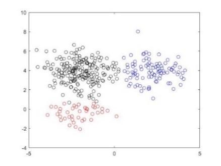
Because $P\left(x_{i} \in[\mu-3 \sigma, \mu+3 \sigma]\right) \approx 99.731 \%$ in Gaussian distribution, each dimension was normalized into the interval [-3, 3]. Then, the clustering results at α=0.100 and H(λ)=N(0, I) were obtained (Figure 2).
The results show that the DPMM automatically divided the sample dataset into three clusters at the accuracy of 95.430 %. Five iterations were completed before the convergence. The parameters estimated from the results are displayed in Table 1 below. It can be seen that the estimated parameters were close to the real parameters.
Figure 2. Results of DPMM
Table 1. Estimated parameters and statistics of the result
|
Cluster number |
Mean of dimension 1 |
Mean of dimension 2 |
Variance of dimension 1 |
Variance of dimension 2 |
The number of elements |
|
1 |
-1.981 |
3.858 |
0.962 |
1.310 |
214 |
|
2 |
2.220 |
3.913 |
0.876 |
1.141 |
95 |
|
3 |
-2.083 |
-0.420 |
0.860 |
0.446 |
41 |
3.2 Rules of parameters
To begin with, a dataset was cited from Reference [23]. Then, the data were normalized into the ranges [-3, 3], [-5, 5] and [-7, 7]. Next, the clustering results of different ranges at α=0.100 and H(λ)=N(0,I) were obtained (Figure 3).
Normalizing range [-3, 3]
Normalizing range [-5, 5]
Normalizing range [-7, 7]
Figure 3. Result of different normalizing ranges with fixed α
Figure 3 reveals an interesting rule that the normalizing range is positively correlated with the number of clusters. To observe the impact of α, the clustering was performed at different values of α but a fixed normalizing range [-5, 5]. The clustering results are shown in Figure 4.
As shown in Figure 4, the number of clusters will be increased by the increasing of α. And a smaller α performs better than a larger one, for a large α can generate a lot of single-point clusters. Thus, to optimize the clustering result, more emphasis should be put on the normalizing range than α, and the latter should be kept at a relatively small value. When normalizing range is [-5, 5] and α=0.100 or α=0.001, each cluster can be marked accurately in different colors, that is, the results are optimized under these two pairs of parameters. In addition, the optimized results also reflect model’s robustness for different parameters at the same time.
α=0.001
α=1
α=1000
Figure 4. Result of different α with fixed normalizing range
As can be seen from Table 2, the mean of each cluster is successfully found, which can represent the center of each cluster.
The above phenomenon can be explained by the rules derived from equation (3). The value of $p\left(\boldsymbol{x}_{i} \in c_{n e w}\right)$ will be increased by the growing of α significantly. This is why a large α can lead to a lot of single-point clusters in the result. When the normalizing range is enlarged, the value of $p\left(\boldsymbol{x}_{i} | \widehat{\boldsymbol{\theta}_{k}}\right)$ for the point far from the center of some existing big clusters will be very small, thus the point has more possibility to fall into the nearest cluster than one big cluster.
Table 2. Estimated parameters and statistics of the best result
|
Cluster number |
Mean of dimension 1 |
Mean of dimension 2 |
Variance of dimension 1 |
Variance of dimension 2 |
The number of elements |
|
1 |
17.420 |
7.180 |
13.821 |
7.751 |
273 |
|
2 |
9.367 |
22.952 |
8.290 |
11.894 |
170 |
|
3 |
32.695 |
22.138 |
3.512 |
9.828 |
128 |
|
4 |
33.143 |
8.793 |
3.405 |
8.296 |
104 |
|
5 |
21.543 |
23.003 |
3.090 |
1.375 |
45 |
|
6 |
7.282 |
11.810 |
1.477 |
1.037 |
34 |
|
7 |
6.517 |
3.541 |
1.115 |
0.715 |
34 |
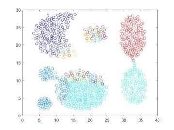
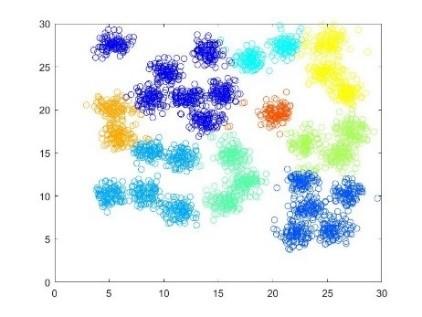
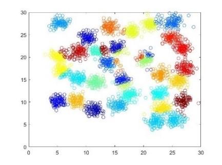
The data set in this part is from Reference [22]. It contains 31 clusters and each cluster has 100 elements. In this sub-section, H(λ)=N(0,I) is still the setting. Firstly, trying range [-5, 5], [-25, 25] and α=0.001. The clustering results are plotted in Figure 5 below.
From Figure 5, there are a lot of undivided clusters for each result. And the second result has too many erroneous small clusters after the normalizing range was increased largely. Thus, continually enlarging the normalizing range goes into invalid for this dataset.
Normalizing range [-5, 5]
Normalizing range [-25, 25]
Figure 5. Clustering result of different normalizing range with fixed α
To solve this problem, these inaccurate big clusters need to be break into several precise small clusters. Here, an algorithm which combines DPMM with the notion of Hierarchical Clustering is raised. The algorithm of Hierarchical DPMM is shown below.
Algorithm 2. Recursion algorithm of Hierarchical DPMM
Input: dataset
Begin
do Algorithm 1 for data set and get a set of clusters $C=$ clustering $(\text {set})$
if size of C equals to 1
do nothing
else
for each ci in C do:
if size of $c_{i}>$ threshold:
do Algorithm 2 for ci
end
end
end
End
Output: the set of data marked by clusters’ number
In this algorithm, one condition for ending the recursion loop is that the size of clustering result equals to one, which means the cluster cannot be separated if it is accurate. However, because the optimal normalizing range and α are different for each cluster’s re-clustering, a constant pair of parameters will lead to the inaccurate dividing in the recursion loop. As the result, Algorithm 1 needs a method that can dynamically produce reasonable parameters for different cluster.
Aiming at the data of this section, two-step normalization is a good way to generate parameters dynamically. First, the original data were normalized to the range [-halfRange, halfRange]. Then, the minimum variance of each dimension was obtained, and taken as the newHalfRange. Finally, the data was normalized again into the range [-newHalfRange, newHalfRange]. The algorithm is shown as below.
Algorithm 3. Two-step Normalization
Input: dataset
Begin
normalize the dataset into the range $[-{halfRange, halfRange}]$ to get newSet
for each column $\mathrm{col}_{j}$ in newSet do:
$\sigma_{j}^{2}=\frac{\sum_{i=1}^{N}\left(x_{i j}-\mu_{j}\right)^{2}}{N}$
end
find the minimum variance $\sigma_{\min }^{2}$
normalize the newSet into the range $\left[-\sigma_{m i n}^{2}, \sigma_{m i n}^{2}\right]$
End
Output: two-step normalized newSet
Another condition to end the recursion loop is a setting of threshold as the minimum number of elements for every cluster. If the amount of points in one cluster is smaller than the threshold, this cluster does not need dividing.
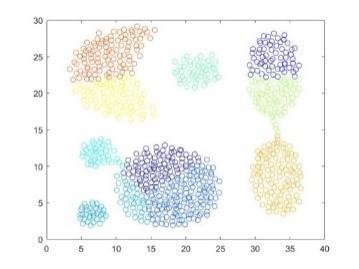
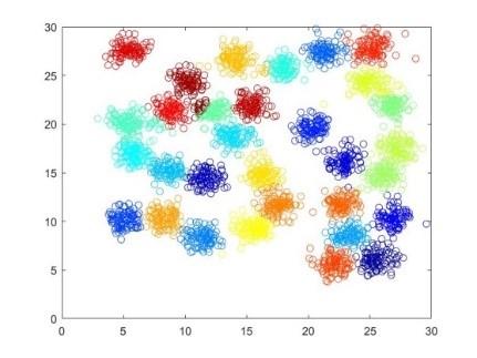
For the case of this section, setting $threshold=200$, $half Range=3.800$ and $\alpha=0.025 \times half Range$. The result of Hierarchical DPMM is shown as follows:
Figure 6. Clustering results of hierarchical DPMM
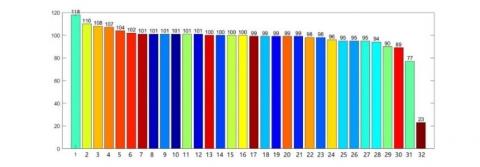
Table 3. Estimated parameters and statistics of first ten clusters
|
Cluster number |
Mean of dimension 1 |
Mean of dimension 2 |
Variance of dimension 1 |
Variance of dimension 2 |
The number of elements |
|
1 |
5.640 |
20.084 |
1.270 |
0.671 |
118 |
|
2 |
24.963 |
24.218 |
0.948 |
0.482 |
110 |
|
3 |
14.170 |
26.633 |
0.897 |
0.678 |
108 |
|
4 |
17.510 |
11.691 |
0.552 |
0.657 |
107 |
|
5 |
22.106 |
5.620 |
0.531 |
0.580 |
104 |
|
6 |
25.191 |
27.827 |
0.821 |
0.709 |
102 |
|
7 |
15.401 |
21.940 |
0.478 |
0.565 |
101 |
|
8 |
11.692 |
14.428 |
0.543 |
0.528 |
101 |
|
9 |
11.368 |
8.337 |
0.553 |
0.539 |
101 |
|
10 |
25.568 |
6.060 |
0.646 |
0.637 |
101 |
From equation (1) to Algorithm 1, this paper provides one path for the realization of the DPMM. Next, three examples were cited to verify the clustering ability of the DPMM algorithm. In the first example, the clustering accuracy reached 95.430 %, and the number of clusters equaled the setting of simulated data. In the second example, the results could be optimized by parameter adjustment, and the normalizing range had more influence on the results than α. In the third example, the DPMM failed to provide accurate results, while the clustering results of hierarchical DPMM were close to the dataset setting. Overall, the three examples can prove the flexibility of the DPMM and the excellent clustering effect of hierarchical DPMM. of course, the hierarchical DPMM also faces the dissimilarity of each sub-cluster in optimal parameters (i.e. normalizing range and α). Thus, the future research will look for a self-adaption method to provide faithful parameters for the DPMM.
We would like to thank the anonymous reviewers for their suggestions to improve this article. This work was supported by National Natural Science Foundation of China (61003130), National Science and Technology Support Program (2012BAH33F03) and Natural Science Foundation of Hubei Province (2015CFB525).
[1] Cui, X.L., Zhu, P.F., Yang, X., Li, K.Q., Ji, C.Q. (2014). Optimized big data K-means clustering using MapReduce. Journal of Supercomputing, 70(3): 1249-1259.
[2] Jain, A.K. (2010). Data clustering: 50 years beyond K-means. Lecture Notes in Computer Science, 5211: 3-4. https://doi.org/10.1007/978-3-540-87479-9_3
[3] Rodriguez, A., Laio, A. (2014). Clustering by fast search and find of density peaks. Science, 344(6191): 1492-1496. https://doi.org/10.1126/science.1242072
[4] Bai, L., Chen, X.Q., Liang, J.Y., Shen, H.W., Guo, Y.K. (2017). Fast density clustering strategies based on the K-means algorithm. Pattern Recognition, 71: 375-386. http://dx.doi.org/10.1016/j.patcog.2017.06.023
[5] Nanda, S.J., Panda, G. (2015). Design of computationally efficient density-based clustering algorithms. Data & Knowledge Engineering, 95: 23-38. https://doi.org/10.1016/j.datak.2014.11.004
[6] Antoniak, C.E. (1974). Mixtures of Dirichlet processes with applications to Bayesian nonparametric problems. Annals of Statistics, 2(6): 1152-1174. http://dx.doi.org/10.1214/aos/1176342871
[7] Escobar, M.D., West, M. (1995). Bayesian density estimation and inference using mixtures. Journal of the American Statistical Association, 90(430): 577-588. http://dx.doi.org/10.1080/01621459.1995.10476550
[8] Shahbaba, B., Neal, R. (2009). Nonlinear models using Dirichlet process mixtures. Journal of Machine Learning Research, 10: 1829-1850. http://dx.doi.org/10.1145/1577069.1755846
[9] Ishwaran, H., Zarepour, M. (2000). Markov chain monte Carlo in approximate Dirichlet and beta two-parameter process hierarchical models. Biometrika, 87(2): 371-390. http://dx.doi.org/10.1093/biomet/87.2.371
[10] Ishwaran, H., James, L.F. (2003). Generalized weighted Chinese restaurant processes for species sampling mixture models. Statistica Sinica, 13(4): 1211-1235.
[11] Raykov, Y.P., Boukouvalas, A., Little, M.A. (2016). Simple approximate MAP inference for Dirichlet processes mixtures. Electronic Journal of Statistics, 10(2): 3548-3578.
[12] Yerebakan, H.Z., Dundar, M. (2017). Partially collapsed parallel Gibbs sampler for Dirichlet process mixture models. Pattern Recognition Letters, 90: 22-27. http://dx.doi.org/10.1016/j.patrec.2017.03.009
[13] Wade, S., Dunson, D.B., Petrone, S., Trippa, L. (2014). Improving prediction from Dirichlet process mixtures via enrichment. Journal of Machine Learning Research, 15: 1041-1071. http://dx.doi.org/10.1016/j.datak.2013.07.003
[14] Liverani, S., Hastie, D.I., Azizi, L., Papathomas, M., Richardson, S. (2015). PReMiuM: An R package for profile regression mixture models using Dirichlet processes. Journal of Statistical Software, 64(7): 1-30. https://doi.org/10.18637/jss.v064.i07
[15] Haines, T.S.F., Xiang, T. (2014). Background subtraction with Dirichlet process mixture models. IEEE Transactions on Pattern Analysis and Machine Intelligence, 36(4): 670-683. https://doi.org/10.1109/TPAMI.2013.239
[16] Sun, X., Yung, N.H.C., Lam, E.Y. (2016). Unsupervised tracking with the doubly stochastic Dirichlet process mixture model. IEEE Transactions on Intelligent Transportation Systems, 17(9): 2594-2599. https://doi.org/10.1109/TITS.2016.2518212
[17] Prabhakaran, S., Rey, M., Zagordi, O., Beerenwinkel, N., Roth, V. (2014). HIV haplptype inference using a propagating Dirichlet process mixture model. IEEE-ACM Transactions on Computational Biology and Bioinformatics, 11(1): 182-191.
[18] Huang, X.L., Hu, F., Wu, J., Chen, H.H., Wang, G., Jiang, T. (2015). Intelligent cooperative spectrum sensing via. IEEE Journal on Selected Areas in Communications, 33(5): 771-787. https://doi.org/10.1109/JSAC.2014.2361075
[19] Murphy, K.P. (2012). Machine Learning: A Probabilistic Perspective. The MIT Press, USA.
[20] Neal, R. (2000). Markov chain sampling methods for Dirichlet process mixture models. Journal of Computational and Graphical Statistics, 9: 249-265. https://doi.org/10.1080/10618600.2000.10474879
[21] Gionis, A., Mannila, H., Tsaparas, P. (2007). Clustering aggregation. ACM Transactions on Knowledge Discovery from Data, 1(1): 1-30. https://doi.org/10.1007/978-0-387-30164-8_125
[22] Veenman, C.J., Reinders, M.J.T., Backer, E. (2002). A maximum variance cluster algorithm. IEEE Transactions Pattern Analysis and Machine Intelligence, 24(9): 1273-1280. https://doi.org/10.1109/TPAMI.2002.1033218