I Gede Agung Krisna Pamungkas | Tohari Ahmad* | Royyana Muslim Ijtihadie
© 2022 IIETA. This article is published by IIETA and is licensed under the CC BY 4.0 license (http://creativecommons.org/licenses/by/4.0/).
OPEN ACCESS
Exchanging data between devices is getting easier and faster just by using a network. Nevertheless, many factors threaten this process and the network itself. Implementing an Intrusion Detection System (IDS) may minimize the risk since it can identify and prevent attacks on the network. There are many methods to design an IDS to work optimally only by reducing data dimensions, one of which is by using the Autoencoder. However, its data dimensions may not have been optimal, which affects the IDS performance. In this study, we work on this problem. This study shows that one of the dimensional reduction methods can get optimal results. It indicates that it is implementable to secure the network.
computer network, intrusion detection system, network infrastructure, network security
Currently, most information is obtained from network technology, from which we can easily access various information and exchange data. Despite its advantages, a network is vulnerable to an attack, where illegal parties may compromise and destroy the data and other resources. Therefore, systems preventing a network from attacks are introduced, one of which is an Intrusion Detection System (IDS) [1, 2] that can identify attack attempts by examining activities in a network or system.
In general, IDS can be divided into host-based and network-based IDS, known as HIDS and NIDS, respectively. HIDS monitors activities where it has been installed. This analysis includes file integrity and finding malicious activities in log files. Slightly different, NIDS focuses on evaluating infrastructure. Analyzing network packets, including headers and contents, makes it feasible to recognize flows for identifying an attack in the network [1].
Furthermore, both IDS types evaluate incoming packets considering either signature-based or anomaly-based mechanisms. In the first approach, detection is done according to existing attacks' defined signatures or rules. The system detects current attacks by comparing their activities with stored signatures without identifying new attack types. The second approach searches for deviation from normal behaviors using machine learning to detect activities [1].
Current IDS is developed using machine learning algorithms focusing on either feature extraction or type classification. For example, Megantara and Ahmad [2] employ feature importance and RFE to extract features, Ahmad and Aziz [3] implement CFS-PSO feature selection, and Muttaqien and Ahmad [4] reduce dimension. In this study, we take Autoencoder to compress data, inspired by Farahnakian and Heikkonen [5], which implement Autoencoder and the Softmax classifier to the KDDCup99 dataset. Autoencoder is a well-known scheme to use in this field [5]. Different from [5] that implements the system in only one dataset, we evaluate the method in four datasets. This has made it easier to analyze the characteristics and environment where the system is more appropriate to implement. Furthermore, we also evaluate several compression sizes to improve the performance further.
The remainder of this paper is organized as follows. Section 2 reviews literature relating to Autoencoder-based feature extraction in IDS. Section 3 explains the method, while Section 4 analyses and compares the experimental results with other methods. Finally, we conclude them in Section 5.
Autoencoder-based feature extraction in IDS has been introduced, such as that proposed by Farahnakian and Heikkonen [5], and Potluri and Diedrich [6]. These two methods [5, 6] compress data using an encoder and then return it using a decoder. The encoder produces data with fewer features than the original one, called code, and the output of the decoder is made as close as possible to its original. Autoencoder has three parts, encoder, decoder, and code. The encoder compresses the input to lower-dimensional output (code), and the decoder generates input from the lower dimensional output produced by the encoder [5]. Overall, the Autoencoder output is not the same as the input because it only translates data. Therefore, a minimal loss is made.
By implementing their method in the KDDCup99 dataset, Farahnakian and Heikkonen [5] transform categorical data using One-Hot Encoding, so the number of features has become more than the original. One-Hot Encoding is a type of mapping converting categorical features into numerical features with binary coding. For example, TCP, UDP, and ICMP are mapped to (1,0,0), (0,1,0), and (0,0,1) [5]. They consider four layers of Autoencoder architecture for feature extraction with (32, 32, 32, 32). They take Softmax by calculating the multiclass and binary classification. Potluri and Diedrich [6] transform categorical data using label encoding in the NSL dataset, where the number of features is the same as the original. Label encoding converting categorical to numerical values. For example, TCP, UDP, and ICMP are converted to 1, 2, and 3, respectively. They also use two layers Autoencoder architecture for feature extraction with (20, 10). Furthermore, Softmax is also implemented by calculating four types of classification. The first is binary classification; the second has three classes with one normal, a type of attacks (i.e., DoS), and one remaining total attack type; the third has three classes with one normal, two types of attacks (i.e., DoS, Probe), and one remaining total attack types; the last comprises one normal and four types of attacks.
By taking the NSL-KDD dataset, Al-Qatf et al. [7] transform categorical data using One-Hot Encoding. They also implement Autoencoder architecture as feature extraction with only one layer. The SVM classifier is implemented by calculating the binary and multiclass classification. The model is evaluated based on training and testing data, and various compression amounts from 10 to 120 are considered. Several Autoencoder-based methods for feature extraction are also proposed, such as [8] using Autoencoder as data compression in the NSL-KDD dataset; [9] using Autoencoder as feature extraction in CICIDS 2017 dataset; and [10] using CNN and LSTM as layer autoencoder for feature extraction. In general, the best architecture is Autoencoder using architecture Stacked-CNN-LSTM-SAE-NN.
Based on those previous studies, it is found that there are many variants of the Autoencoder implementation based on the number of layers, the type of classification, and the used dataset. However, previous research still needs to be evaluated using different parameters to improve its performance. Furthermore, some metrics should also be implemented to measure that performance further.
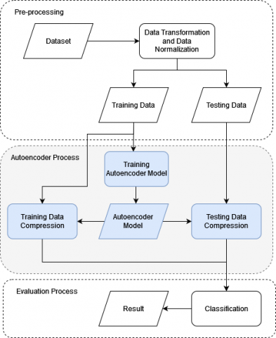
Figure 1. Stages of the proposed method
In this research, the Autoencoder reduces the number of features by 75%, 50%, and 25%. Those percentages are chosen because these values represent various data sizes with reasonable differences. The main process flow is described as follows:
Pre-processing: We use One-Hot-Encoder to convert categorical data into numerical data for preprocessing. Then, data are normalized using MinMaxScaler.
Autoencoder Process: The Autoencoder model is trained to produce this model. The next is to compress data training and testing with that Autoencoder.
Evaluation Process: The data evaluation uses Softmax, k-NN, and Naïve Bayes classification.
Each stage of this scheme is illustrated in Figure 1. The focus of this experiment is the Autoencoder process, where we compress the data in different amounts, namely 25%, 50%, and 75% for each dataset, whose process is described as follows.
3.1 Preprocessing
In this stage, first, we convert categorical data using One-Hot-Encoder, a method to transform categorical data to numerical with binary coding. It results in 0 or 1, representing "not in this category" and "in a category", respectively. After converting to numerical features, all datasets have more features. The NSL-KDD dataset is from 41 to 122, UNSW-NB15 is from 42 to 196, KDDCup99 is from 41 to 119, and Kyoto is from 23 to 46. Next, all datasets are normalized with MinMaxScaler to make 0 to 1.
3.2 Autoencoder process
After preprocessing data, we create an Autoencoder model by compressing all features to 75%, 50%, and 25%. Each compressed ratio creates a different layer, so we have nine models consisting of 75% one-layer, two-layer, three-layer; 50% one-layer, two-layer, three-layer; 25% one-layer, two-layer, three-layer
The process starts by training the first Autoencoder with training data and compressing. Then, training the second Autoencoder with compressed data in the first Autoencoder creates the compression. Last, train the third Autoencoder with compressed data in the second Autoencoder.
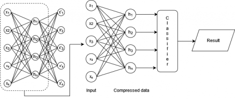
Figure 2. Autoencoder model
After Autoencoder was trained, we have 3 Autoencoders: the first Autoencoder is one layer, the first to second Autoencoder is a two-layer, and the first to third Autoencoder is a three-layer. Those are trained again with different compressed ratios. Compressing data training and testing with trained Autoencoder, which is used for classification, produces fewer features than the original. Figure 2 shows an autoencoder model consisting of 3 layers, each of which is trained with a different autoencoder.
3.3 Evaluation process
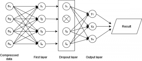
The compressed data are evaluated using Softmax, k-NN, and Naïve Bayes Classification. Softmax classifier expands the Logistic Regression (LR) method that LR only categories two labels. On the other hand, Softmax extends it into multi-category labels; this characteristic is more appropriate to implement for multiclass environments. Furthermore, Softmax can be applied to map N-dimensional vectors into categories [11]. For Softmax classification, we use 100 batches for training with Binary Crossentropy loss and Adam Optimizer, whose architecture contains two layers. In the first layer, the number of neurons is the same as the number of compressed features, and in the output layer, the number of neurons is the same as the number of classifications. After the first layer, we perform the dropout layer for combat overfitting. The classification architecture is shown in Figure 3.
Figure 3. Softmax classification model
The k-NN algorithm is a supervised learning method by storing previous data and classifying incoming data according to its distance to those previous ones, and the close neighborhood of k is checked. The incoming data are included in their closest class by measuring the Euclidean, Minkowski, or Manhattan to find the distance [12]. On the other hand, Naïve Bayes classifies data according to the probabilistic values in the Bayes theorem and the naïve independence assumptions. The algorithm consolidates the existence of a specific feature that is irrelevant to the current environment. As a supervised learning method, it is trained for small data sets to detect many attributes later [13]. This environment has been considered based on the previous supervised and unsupervised learning comparison [14].
In the experiment, we used four datasets, namely NSL-KDD, UNSW-NB15, Kyoto, and KDDCup99, to get diverse comparisons. Furthermore, multiclass and binary classifications are performed whenever the dataset supports it (e.g., the Kyoto dataset is binary only). Like other research, we generate a confusion matrix containing True Positive (TP), True Negative (TN), False Positive (FP), and False Negative (FN) to find the True Positive Rate (TPR) and the False Negative Rate (FPN) of the experimental results. TP is the number of correctly detected attacks, TN is the number of correctly detected normal, FP is the number of normal detected as an attack, and FN is attack detected as normal.
For the NSL-KDD dataset, we use KDDTrain+.txt as training and KDDTest+.txt as testing with 125973 and 22544 data, respectively. NSL-KDD has 23 classes and is reduced to 5 classes with one normal and four attacks (Denial of Service (DoS), Use to Root (U2R), Remote to Local (R2L), and Probe. As for the Kyoto dataset, we use 20151231.txt as the dataset with a total data size of 309068 data. It has two classes with a value of 1 as normal and a -1 as an attack. For the UNSW-NB15 dataset, we use UNSW_NB15_training-set.csv for training, and UNSW_NB15_testing-set.csv for testing with a total of 82332 and 175341 data, respectively. The UNSW-NB15 dataset has ten classes with one normal and nine attacks (Analysis, Backdoor, DoS, Exploits, Fuzzers, Generic, Reconnaissance, Shellcode, and Worms). In the KDDCup99 Dataset, kddcup.data_10_percent_corrected is taken for training and corrected for data testing containing 494021 and 311029 for data training and testing, respectively. This dataset has redundant data; we reduced it to 145586 and 77291 data.
4.1 Difference number of hidden layers and hidden units
We use an Autoencoder with three amounts of compression, namely 25%, 50%, and 75%. Furthermore, we also implement several layers, from one to three, as described in the following scenarios.
4.1.1 Scenario 1
We compress data using Autoencoder to 25% for each dataset. In the NSL-KDD, the number of features reduces from 122 to 30; in the UNSW-NB15, it is from 196 to 49; the Kyoto dataset is from 46 to 11; lastly, for KDDCup99, the number goes down from 119 to 30. In this scenario, the highest accuracy on multiclass classification is 93.40% in 3 layers with Softmax and KDDCup99 datasets, while that in binary is 98.79% in 3 layers with k-NN and Kyoto datasets. The results are provided in Table 1, where B, M, and k are the binary classification, multiclass classification, and the number of nearest neighbors in k-NN, respectively. The sensitivity (SE) and specificity (SP) in binary and multiclass classification are shown in Table 2 and Table 3, respectively. It is shown that, overall, in terms of SE, Softmax and Naive Bayes are more appropriate to the multiclass environment. However, their SP values are comparable, depending on the dataset. In the binary classification, k-NN applied to the Kyoto and KDDCup99 dataset has the highest SE and SP values, respectively. For the multiclass, Softmax applied to UNSW-NB15 and k-NN with KDDCup99 datasets have the best SE and SP values, respectively.
4.1.2 Scenario 2
Unlike scenario 1, in scenario 2, we make the Autoencoder compression of 50% for each dataset. Here, the highest accuracy on multiclass is 93.16% in 3 layers with Softmax and KDDCup99 datasets, and that of binary is 99.00% in 1 layer with Softmax and Kyoto datasets. In this scenario, the experimental results are provided in Tables 4, 5, and 6. In general, this scenario produces similar patterns to the previous scenario 1.
4.1.3 Scenario 3
In the last scenario, we make the Autoencoder compression amount of 75% for each dataset. In scenario 3, the highest accuracy on multiclass classification is obtained using one layer with Softmax and KDDCup99 datasets, 93.55%; and that of binary is in 1 layer with Softmax and Kyoto datasets, which is 99.42%. Tables 7, 8, and 9 show the detail of the results. Same as scenario 2, this experiment shows similar patterns to scenario 1.
Table 1. The accuracy using 25% compression (B=binary, M=multiclass, k=nearest neighbors)
|
Layer |
Softmax Layer (%) |
k-NN Classification (%) for specified k |
Naïve Bayes Classification (%) |
|||||
|
B |
M |
k |
B |
k |
M |
B |
M |
|
|
NSL-KDD Dataset |
||||||||
|
1 |
75.16 |
78.15 |
37 |
79.78 |
37 |
78.19 |
75.12 |
62.49 |
|
2 |
79.36 |
82.78 |
29 |
80.05 |
29 |
78.60 |
75.20 |
61.40 |
|
3 |
75.23 |
80.69 |
23 |
80.12 |
29 |
78.50 |
76.50 |
63.52 |
|
UNSW-NB15 Dataset |
||||||||
|
1 |
85.99 |
67.21 |
3 |
88.31 |
5 |
72.02 |
73.81 |
58.75 |
|
2 |
90.20 |
67.35 |
3 |
88.17 |
7 |
71.93 |
73.92 |
55.26 |
|
3 |
86.05 |
66.89 |
3 |
88.06 |
13 |
71.31 |
74.07 |
58.47 |
|
Kyoto Dataset |
||||||||
|
1 |
98.53 |
- |
5 |
98.60 |
- |
- |
85.06 |
- |
|
2 |
97.14 |
- |
5 |
98.66 |
- |
- |
92.35 |
- |
|
3 |
97.52 |
- |
5 |
98.79 |
- |
- |
96.09 |
- |
|
KDDCup99 Dataset |
||||||||
|
1 |
94.27 |
92.37 |
41 |
94.38 |
3 |
9265.00 |
91.03 |
87.35 |
|
2 |
94.31 |
92.50 |
41 |
94.57 |
3 |
92.95 |
90.68 |
86.53 |
|
3 |
94.25 |
93.40 |
41 |
94.61 |
3 |
92.86 |
90.36 |
77.82 |
Table 2. Sensitivity (SE) and specificity (SP) of binary classification using 25% compression
|
Layer |
Softmax Layer |
k-NN Classification |
Naïve Bayes Classification |
|||
|
SE (%) |
SP (%) |
SE (%) |
SP (%) |
SE (%) |
SP (%) |
|
|
NSL-KDD Dataset |
||||||
|
1 |
62.06 |
92.48 |
70.34 |
92.25 |
63.04 |
91,09. |
|
2 |
67.26 |
95.36 |
70.78 |
92.30 |
62.97 |
91.36 |
|
3 |
61.90 |
92.84 |
70.86 |
92.36 |
65.38 |
91.20 |
|
UNSW-NB15 Dataset |
||||||
|
1 |
80.62 |
97.43 |
85.02 |
95.31 |
63.99 |
94.72 |
|
2 |
88.6 |
93.60 |
84.94 |
95.06 |
64.16 |
94.71 |
|
3 |
80.67 |
97.51 |
84.83 |
94.94 |
64.45 |
94.58 |
|
Kyoto Dataset |
||||||
|
1 |
99.88 |
74.41 |
99.43 |
80.77 |
85.27 |
80.50 |
|
2 |
97.89 |
81.09 |
99.40 |
82.62 |
92.93 |
79.64 |
|
3 |
98.34 |
79.77 |
99.52 |
82.94 |
96.9 |
78.6 |
|
KDDCup99 Dataset |
||||||
|
1 |
87.84 |
98.20 |
86.55 |
99.18 |
79.37 |
98.17 |
|
2 |
88.58 |
97.83 |
87.02 |
99.20 |
78.12 |
98.38 |
|
3 |
88.01 |
98.07 |
87.10 |
99.22 |
75.79 |
99.29 |
Table 3. Sensitivity (SE) and specificity (SP) of multiclass classification using 25% compression
|
Layer |
Softmax Layer |
k-NN Classification |
Naïve Bayes Classification |
|||
|
SE (%) |
SP (%) |
SE (%) |
SP (%) |
SE (%) |
SP (%) |
|
|
NSL-KDD Dataset |
||||||
|
1 |
77.32 |
91.16 |
70.18 |
92.26 |
67.79 |
87.92 |
|
2 |
80.02 |
94.77 |
70.67 |
92.33 |
69.54 |
90.64 |
|
3 |
77.13 |
95.43 |
70.57 |
92.37 |
70.86 |
86.86 |
|
UNSW-NB15 Dataset |
||||||
|
1 |
98.95 |
80.23 |
83.96 |
96.15 |
96.73 |
77.03 |
|
2 |
99.16 |
80.36 |
82.67 |
96.61 |
97.55 |
78.92 |
|
3 |
99.01 |
80.25 |
80.46 |
97.47 |
96.33 |
78.68 |
|
KDDCup99 Dataset |
||||||
|
1 |
91.40 |
97.33 |
85.92 |
98.36 |
86.04 |
95.16 |
|
2 |
91.85 |
96.99 |
85.73 |
99.13 |
87.98 |
93.86 |
|
3 |
92.82 |
97.31 |
86.11 |
99.11 |
86.33 |
96.17 |
Table 4. The accuracy using 50% compression (B=binary, M=multiclass, k=nearest neighbors)
|
Layer |
Softmax Layer (%) |
k-NN Classification (%)for specified k |
Naïve Bayes Classification (%) |
|||||
|
B |
M |
k |
B |
k |
M |
B |
M |
|
|
NSL-KDD Dataset |
||||||||
|
1 |
76.58 |
78.19 |
21 |
77.47 |
37 |
75.98 |
77.76 |
66.57 |
|
2 |
78.03 |
79.05 |
21 |
77.45 |
21 |
76.11 |
78.72 |
62.81 |
|
3 |
77.10 |
80.86 |
23 |
78.93 |
23 |
77.63 |
76.61 |
76.40 |
|
UNSW-NB15 Dataset |
||||||||
|
1 |
89.42 |
68.40 |
3 |
88.46 |
5 |
72.44 |
74.36 |
55.09 |
|
2 |
89.26 |
68.18 |
3 |
88.27 |
7 |
72.20 |
73.89 |
55.38 |
|
3 |
89.11 |
67.99 |
3 |
88.22 |
13 |
72.14 |
74.00 |
54.25 |
|
Kyoto Dataset |
||||||||
|
1 |
99.00 |
- |
3 |
98.47 |
- |
- |
84.27 |
- |
|
2 |
98.84 |
- |
3 |
98.25 |
- |
- |
84.79 |
- |
|
3 |
98.29 |
- |
3 |
98.08 |
- |
- |
86.06 |
- |
|
KDDCup99 Dataset |
||||||||
|
1 |
93.76 |
92.21 |
41 |
93.95 |
3 |
93.11 |
90.78 |
87.10 |
|
2 |
92.41 |
92.69 |
41 |
93.56 |
3 |
93.13 |
90.75 |
86.29 |
|
3 |
92.78 |
93.16 |
41 |
93.81 |
3 |
93.39 |
90.42 |
86.71 |
Table 5. Sensitivity (SE) and specificity (SP) of binary classification using 50% compression
|
Layer |
Softmax Layer |
k-NN Classification |
Naïve Bayes Classification |
|||
|
SE (%) |
SP (%) |
SE (%) |
SP (%) |
SE (%) |
SP (%) |
|
|
NSL-KDD Dataset |
||||||
|
1 |
64.88 |
92.05 |
66.00 |
92.63 |
67.89 |
90.80 |
|
2 |
63.67 |
97.01 |
65.92 |
92.68 |
69.47 |
90.95 |
|
3 |
64.02 |
94.39 |
65.85 |
96.23 |
65.36 |
91.48 |
|
UNSW-NB15 Dataset |
||||||
|
1 |
85.97 |
96.77 |
85.24 |
95.31 |
64.81 |
94.71 |
|
2 |
85.79 |
96.64 |
85.11 |
94.99 |
64.10 |
94.72 |
|
3 |
85.64 |
96.50 |
85.05 |
94.96 |
64.28 |
94.70 |
|
Kyoto Dataset |
||||||
|
1 |
99.49 |
88.50 |
99.12 |
84.25 |
84.30 |
83.57 |
|
2 |
99.27 |
89.59 |
98.89 |
84.48 |
84.76 |
85.43 |
|
3 |
98.76 |
88.10 |
98.69 |
84.93 |
86.16 |
83.71 |
|
KDDCup99 Dataset |
||||||
|
1 |
84.90 |
99.20 |
85.28 |
99.26 |
77.78 |
98.76 |
|
2 |
82.71 |
98.36 |
85.01 |
98.80 |
77.80 |
98.69 |
|
3 |
84.32 |
97.96 |
85.49 |
98.90 |
77.14 |
98.56 |
Table 6. Sensitivity (SE) and specificity (SP) of multiclass classification using 50% compression
|
Layer |
Softmax Layer |
k-NN Classification |
Naïve Bayes Classification |
|||
|
SE (%) |
SE (%) |
SE (%) |
||||
|
NSL-KDD Dataset |
||||||
|
1 |
77.05 |
90.99 |
65.92 |
92.66 |
74.92 |
90.51 |
|
2 |
74.41 |
95.37 |
65.87 |
92.68 |
71.85 |
88.52 |
|
3 |
76.22 |
95.59 |
65.82 |
96.24 |
72.94 |
93.37 |
|
UNSW-NB15 Dataset |
||||||
|
1 |
99.24 |
80.22 |
84.32 |
96.03 |
96.34 |
72.13 |
|
2 |
99.02 |
80.46 |
83.10 |
96.52 |
97.79 |
76.00 |
|
3 |
98.95 |
80.47 |
81.20 |
97.33 |
94.95 |
75.31 |
|
KDDCup99 Dataset |
||||||
|
1 |
88.58 |
97.17 |
85.37 |
99.16 |
87.73 |
95.01 |
|
2 |
89.82 |
97.22 |
84.91 |
99.15 |
87.57 |
93.87 |
|
3 |
91.49 |
97.24 |
85.80 |
99.16 |
86.72 |
95.09 |
Table 7. The accuracy using 75% compression (B=binary, M=multiclass, k=nearest neighbors)
|
Layer |
Softmax Layer (%) |
k-NN Classification (%)for specified k |
Naïve Bayes Classification (%) |
|||||
|
B |
M |
k |
B |
k |
M |
B |
M |
|
|
NSL-KDD Dataset |
||||||||
|
1 |
78.24 |
79.80 |
9 |
76.93 |
9 |
75.70 |
80.20 |
66.19 |
|
2 |
79.32 |
78.72 |
37 |
78.11 |
37 |
76.73 |
79.64 |
70.48 |
|
3 |
77.67 |
79.46 |
39 |
78.18 |
37 |
76.82 |
80.64 |
72.46 |
|
UNSW-NB15 Dataset |
||||||||
|
1 |
87.97 |
67.52 |
3 |
88.64 |
5 |
72.60 |
73.93 |
55.13 |
|
2 |
89.19 |
68.19 |
3 |
88.48 |
7 |
72.60 |
73.78 |
56.01 |
|
3 |
88.41 |
69.24 |
3 |
88.38 |
13 |
72.22 |
73.66 |
56.75 |
|
Kyoto Dataset |
||||||||
|
1 |
99.42 |
- |
3 |
98.69 |
- |
- |
84.24 |
- |
|
2 |
99.12 |
- |
3 |
98.60 |
- |
- |
83.55 |
- |
|
3 |
98.78 |
- |
3 |
97.87 |
- |
- |
84.96 |
- |
|
KDDCup99 Dataset |
||||||||
|
1 |
92.81 |
93.55 |
41 |
93.95 |
3 |
92.76 |
91.37 |
87.13 |
|
2 |
93.05 |
93.13 |
41 |
93.99 |
3 |
93.05 |
91.68 |
86.54 |
|
3 |
92.65 |
92.97 |
41 |
93.87 |
3 |
93.39 |
90.26 |
87.66 |
Table 8. Sensitivity (SE) and specificity (SP) of binary classification using 75% compression
|
Layer |
Softmax Layer |
k-NN Classification |
Naïve Bayes Classification |
|||
|
SE (%) |
SP (%) |
SE (%) |
SP (%) |
SE (%) |
SP (%) |
|
|
NSL-KDD Dataset |
||||||
|
1 |
65.84 |
94.63 |
64.94 |
92.78 |
69.04 |
94.94 |
|
2 |
66.14 |
96.74 |
67.07 |
92.69 |
71.34 |
90.62 |
|
3 |
66.35 |
92.63 |
67.28 |
92.60 |
73.75 |
89.74 |
|
UNSW-NB15 Dataset |
||||||
|
1 |
83.55 |
97.40 |
85.47 |
95.40 |
64.37 |
94.29 |
|
2 |
85.63 |
96.78 |
85.43 |
94.99 |
63.94 |
94.74 |
|
3 |
84.23 |
97.30 |
85.30 |
94.94 |
63.77 |
94.73 |
|
Kyoto Dataset |
||||||
|
1 |
99.95 |
89.86 |
99.36 |
84.30 |
84.27 |
83.66 |
|
2 |
99.61 |
88.50 |
99.28 |
83.85 |
83.54 |
83.66 |
|
3 |
99.27 |
88.10 |
98.54 |
83.35 |
85.01 |
83.94 |
|
KDDCup99 Dataset |
||||||
|
1 |
83.86 |
98.30 |
85.26 |
99.28 |
77.94 |
99.60 |
|
2 |
84.41 |
98.35 |
85.38 |
99.27 |
80.87 |
98.31 |
|
3 |
83.39 |
98.32 |
85.28 |
99.40 |
74.95 |
99.64 |
Table 9. Sensitivity (SE) and specificity (SP) of multiclass classification using 75% compression
|
Layer |
Softmax Layer |
k-NN Classification |
Naïve Bayes Classification |
|||
|
SE (%) |
SE (%) |
SE (%) |
||||
|
NSL-KDD Dataset |
||||||
|
1 |
76.08 |
95.03 |
64.81 |
92.79 |
74.02 |
90.81 |
|
2 |
78.63 |
95.37 |
67.05 |
92.69 |
75.90 |
88.78 |
|
3 |
77.03 |
95.51 |
67.26 |
92.63 |
75.33 |
87.32 |
|
UNSW-NB15 Dataset |
||||||
|
1 |
98.95 |
80.40 |
84.54 |
96.06 |
97.13 |
70.10 |
|
2 |
99.04 |
80.57 |
83.58 |
96.47 |
96.64 |
79.13 |
|
3 |
99.14 |
80.50 |
81.80 |
97.37 |
97.31 |
76.13 |
|
KDDCup99 Dataset |
||||||
|
1 |
90.60 |
97.82 |
85.28 |
98.41 |
87.56 |
95.12 |
|
2 |
90.99 |
97.60 |
85.60 |
98.59 |
89.19 |
93.62 |
|
3 |
87.26 |
98.28 |
85.80 |
99.22 |
86.72 |
95.09 |
4.2 Analysis of 3 scenarios
Generally, the increasing the compression proportionally increases the performance. This specifically works on the accuracy of using Softmax and Naïve Bayes classifiers, for both binary and multiclass classification in NSL-KDD dataset. Using k-NN in the same dataset causes the accuracy reduces gradually. Softmax and k-NN can be used for both binary and multiclass with accuracy around 80% at maximum. On the contrary, Naïve Bayes has about 14% difference of accuracy generated by binary and multiclass. So, it may not be applicable for mutliclass classification at any layer. In this NSL-KDD dataset, the best accuracy in binary classification is scenario 3 with three layers, using Naive Bayes reaching 80.64%. In multiclass classification, scenario 1 with two layers using the Softmax classifier obtains 82.78%. Next, in the UNSW-NB15 dataset, the best accuracy in binary classification is scenario 1 with two layers and using Softmax classification, 90.20%. In comparison, that in multiclass classification is scenario 3 with 1 and 2 layers, using k-NN classification, which is 90.20%.
In the UNSW-NB15 dataset, a relatively large difference between binary and multiclass occurs in all classifiers, where Naïve Bayes still has the highest difference. Here, multiclass classification results are lower than that in NSL-KDD. However, the binary classification results for Softmax and k-NN go up significantly.
As for the Kyoto dataset, there is only binary data, therefore multiclass cannot be evaluated. The experimental results show that the accuracy is higher than that of other datasets. Moreover, the 75% compression can reach 99.42% of accuracy in 1 layer of Softmax. The accuracy in KDDCup99 is lower than that of Kyoto but still higher than others. The change of layer numbers and compression may not much affect the results. The best binary classification in this Kyoto dataset is scenario 3 with one layer, using the Softmax classifier, 99.42%. Lastly, in the KDDCup99 dataset using binary classification, scenario 1 with three layers with k-NN, 94.61%, while in multi-classification is scenario 3 with one layer implementing Softmax, 93.55%.
From those three scenarios, the best result in multiclass is the one layer-Autoencoder on the KDDCup99 dataset, reducing the features to 75%. In binary class, the best result is generated by 1 layer-Autoencoder on the Kyoto dataset, decreasing the features to 75%.
4.3 Comparison with other evaluations
Table 10. Multiclass classification results
|
Methods |
Dataset |
Accuracy (%) |
Sensitivity (%) |
Specificity (%) |
|
DAE-IDS [5] |
KDDCup99 |
94.71 |
94.42 |
- |
|
DNN-IDS [6] |
NSL-KDD |
- |
97.50 |
95.00 |
|
SAE-SVM [7] |
NSL-KDD |
80.48 |
68.29 |
- |
|
Proposed method |
KDDCup99 |
93.55 |
90.63 |
97.82 |
Table 11. Binary classification results
|
Methods |
Dataset |
Accuracy (%) |
Sensitivity (%) |
Specificity (%) |
|
DAE-IDS [5] |
KDDCup99 |
96.53 |
95.65 |
- |
|
DNN-IDS [6] |
NSL-KDD |
- |
97.50 |
96.50 |
|
SAE-SVM [7] |
NSL-KDD |
84,.6 |
76.57 |
- |
|
Proposed method |
Kyoto |
99.42 |
99.95 |
89.86 |
We compare the proposed method [5-7], as shown in Tables 10 and 11 for multiclass and binary classification, respectively. From those tables, we find that binary classification is the best among other methods, with an accuracy of 99.42%, sensitivity of 99.95%, and specificity of 89.86%. However, its specificity is less than that of the study [6]. Imbalanced data likely cause in the Kyoto dataset that the number of attacks is more than the normal. In multiclass classification, the study [5] is the best with accuracy and sensitivity of 94.71% and 94.42% in the KDDCup99 dataset, where the proposed method has 93.55% and 90.63%, respectively. It is possible because the normal is more than the attacks, and the framework neural network is different from the other research.
It is found that the proposed method can produce better results in the Kyoto dataset for binary classification. Meanwhile, the multiclass classification in KDDCup99 is considerable, less than that in the study [5]. This research also shows that the Naive Bayes is less suitable for multiclass classification than k-NN and Softmax. Adding layers to the Autoencoder does not significantly improve performance, as shown by their accuracy. Furthermore, using Autoencoder can reduce computation because the number of features decreases. Nevertheless, this study has not been implemented to specific datasets, which may have different characteristics.
In future research, the performance may be improved by implementing other classifiers. Moreover, some feature selection algorithms can be combined to obtain the best features. To improve the analysis results, differences between compression sizes should be reduced, for example to 5%, so more detailed data can be obtained. Nevertheless, this reduction causes longer time because more data must be processed. More datasets should be taken to evaluate the methods, so that the analysis can be done deeper.
The authors gratefully acknowledge financial support from the Institut Teknologi Sepuluh Nopember for this work, under project scheme of the Publication Writing and IPR Incentive Program (PPHKI) 2022.
[1] Warzyński, A., Kołaczek, G. (2018). Intrusion detection systems vulnerability on adversarial examples. In 2018 Innovations in Intelligent Systems and Applications (INISTA), pp. 1-4. https://doi.org/10.1109/INISTA.2018.8466271
[2] Megantara, A.A., Ahmad, T. (2020). Feature importance ranking for increasing performance of intrusion detection system. In 2020 3rd International Conference on Computer and Informatics Engineering (IC2IE), pp. 37-42. https://doi.org/10.1109/IC2IE50715.2020.9274570
[3] Ahmad, T., Aziz, M.N. (2019). Data preprocessing and feature selection for machine learning intrusion detection systems. ICIC Express Lett, 13(2): 93-101. https://doi.org/10.24507/icicel.13.02.93
[4] Muttaqien, I.Z., Ahmad, T. (2016). Increasing performance of IDS by selecting and transforming features. In 2016 IEEE International Conference on Communication, Networks and Satellite (COMNETSAT), pp. 85-90. https://doi.org/10.1109/COMNETSAT.2016.7907422
[5] Farahnakian, F., Heikkonen, J. (2018). A deep auto-encoder based approach for intrusion detection system. In 2018 20th International Conference on Advanced Communication Technology (ICACT), pp. 178-183. https://doi.org/10.23919/ICACT.2018.8323688
[6] Potluri, S., Diedrich, C. (2016). Accelerated deep neural networks for enhanced intrusion detection system. In 2016 IEEE 21st International Conference on Emerging Technologies and Factory Automation (ETFA), pp. 1-8. https://doi.org/10.1109/ETFA.2016.7733515
[7] Al-Qatf, M., Lasheng, Y., Al-Habib, M., Al-Sabahi, K. (2018). Deep learning approach combining sparse autoencoder with SVM for network intrusion detection. IEEE Access, 6: 52843-52856. https://doi.org/10.1109/ACCESS.2018.2869577
[8] Ieracitano, C., Adeel, A., Morabito, F.C., Hussain, A. (2020). A novel statistical analysis and autoencoder driven intelligent intrusion detection approach. Neurocomputing, 387: 51-62. https://doi.org/10.1016/j.neucom.2019.11.016
[9] Thakur, S., Chakraborty, A., De, R., Kumar, N., Sarkar, R. (2021). Intrusion detection in cyber-physical systems using a generic and domain specific deep autoencoder model. Computers & Electrical Engineering, 91: 107044. https://doi.org/10.1016/j.compeleceng.2021.107044
[10] D’Angelo, G., Palmieri, F. (2021). Network traffic classification using deep convolutional recurrent autoencoder neural networks for spatial–temporal features extraction. Journal of Network and Computer Applications, 173: 102890. https://doi.org/10.1016/j.jnca.2020.102890
[11] Wang, Z., Liu, Y., He, D., Chan, S. (2021). Intrusion detection methods based on integrated deep learning model. Computers & Security, 103: 102177. https://doi.org/10.1016/j.cose.2021.102177
[12] Kilincer, I.F., Ertam, F., Sengur, A. (2021). Machine learning methods for cyber security intrusion detection: Datasets and comparative study. Computer Networks, 188: 107840. https://doi.org/10.1016/j.comnet.2021.107840
[13] Wang, K. (2019). Network data management model based on Naïve Bayes classifier and deep neural networks in heterogeneous wireless networks. Computers & Electrical Engineering, 75: 135-145. https://doi.org/10.1016/j.compeleceng.2019.02.015
[14] Sirisha, A., Chaitanya, K., Krishna, K.V.S.S.R., Kanumalli, S.S. (2021). Intrusion detection models using supervised and unsupervised algorithms - a comparative estimation. International Journal of Safety and Security Engineering, 11(1): 51-58. https://doi.org/10.18280/ijsse.110106