Kalyani Sunkara* | Venkata Rao K | Mary Sowjanya A
© 2021 IIETA. This article is published by IIETA and is licensed under the CC BY 4.0 license (http://creativecommons.org/licenses/by/4.0/).
OPEN ACCESS
Technology of Internet of Things (IoT) offers extensive applications for industrial productivity and safety improvement. Advanced miniature sensors are available for monitoring multiple process parameters in a complex industrial or an engineering system. An industrial plant's overall operational status is captured using a network of sensors and stored on a cloud storage platform, where it is evaluated using the machine learning algorithms to produce valuable insights. Finding the correlation among these sensor variables is essential before feeding the same to machine learning algorithms. The present study proposes a novel approach to choose a few critical sensors out of numerous sensors based on the Response Relationship methodology. The Response Relationship method enables the system to be fully autonomous and helps find the interrelation among variables. The Response Relationship among variables is quantified and used for calculating the Remaining Useful Life of a complex engineering system. The proposed methodology is also applied to binary and multi-class classification to demonstrate the efficiency of the Response Relationship method. The results obtained are compared with standard methods of prediction and classification in terms of suitable metrics.
remaining useful life, sensors, binary classification, multi-class classification, response relationship
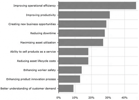
The Internet of Things (IoT) connects multiple machines and devices to the Internet in order to monitor their normal operation, aberrant operation, and the remaining useful life. The development of intelligent machines in aerospace, defense, and automotive needs frameworks that are self-powered and intelligent. With the advancement of cloud storage and processing capabilities, algorithms that run on edge devices offer increased benefits. There are numerous advantages to applying the IoT to manufacturing and engineering products. Figure 1 depicts the benefits of IoT applications like improving operational efficiency, improving safety, improving productivity, improving the well-being of workers, and creating new business opportunities. The application of IoT platforms has demonstrated less frequent downtime, asset planning and scheduling. These platforms can also learn from the product’s features from previously manufactured components and help develop process planning.
With the wide range of enhanced network access, capturing the essential data with sensors and storing it on a cloud storage platform has become much easier. It is estimated that there is an exponential growth in the number of devices connected and consequently the data to be stored proportionally increased giving rise to a new set of challenges for enterprises to make real-world things. In time-critical situations, the stored data may not be helpful if the analysis is delayed due to limited network availability or overloaded central systems. An extensive array of analytics, networking, storage, high computation power, and suitable infrastructure are essential to analyze large amounts of data.
In finance, insurance, and other closely related industries, generated data is examined using both conventional methods and models created during the last few decades. Though analytics is essential to IoT’s rapid growth and business value, conventional analytics approach may not fulfill different applications. Usually, such models cannot be directly used for sensor data analysis. Developing separate IoT application models is therefore highly essential. As sensors are located at various conditions, a new framework is required, which is applicable for industrial equipment. Data analysis techniques for analyzing the data captured in such platforms must therefore be improved and moved to edge devices to process the information efficiently. The primary challenge is to identify the most relevant predictors that will help predict each target time series. The current research presents a feature selection technique for multivariate time series forecasting.
The paper’s remaining section is structured as follows: Section 2 reviews the recent developments in feature engineering and feature selection aspects to estimate the Remaining Useful Life of complex engineering systems. Section 3 describes the dataset used and its exploratory data analysis, followed by the proposed methodology in Section 4. Section 5 presents the Experimental study, results obtained, and discussions. Finally, the conclusion and future work is presented in Section 6.
Figure 1. Advantages of industrial IoT
Data-Driven Modeling has increased momentum with huge growth of articles utilising a variety of algorithms. Yan and Zhang [1] proposed a method for analysing and selecting features from correlated gas sensor data. To achieve a promising performance, this model's recursive feature removal technique used a correlation bias reduction strategy with linear and nonlinear SVM-RFE algorithms. Day et al. [2] presented the concept of autonomic feature selection through the lens of two concepts: representation and transfer learning. A system's representations for various forms of monitoring data are learnt, and the resulting knowledge is shared and reused. Su et al. [3] investigated the sensor data's feature engineering elements. Their approach entailed gathering sensor data correlation changes in order to enhance the detection of IoT (Internet of Things) equipment anomalies. Mosallam et al. [4] established a comprehensive foundation for RUL Prediction that is applicable to a wide variety of issues via the Bayesian approach. Li et al. [5] proposed a novel promising strategy for remaining useful life projections that requires no prior experience or signal processing. They used a deep convolutional neural network-based method. They examined the effect of critical factors on model parameter optimization for prognostic performance. Yu et al. [6] established a cluster-based data analysis framework based on recursive principal component analysis (R-PCA) that aggregates correlated sensor data fast and accurately with outlier identification. Hromic et al. [7] extended the OpenIoTmiddleware's functionality for stream processing, providing real-time demand analytics on data streams. Ren et al. [8] proposed an integrated deep neural network approach for estimating the remaining useful life of a rolling bearing by combining time domain and frequency domain information. Le Son et al. [9] described a probabilistic approach to prognosis by integrating a data analysis technique (Principal Component Analysis) with a stochastic process (Wiener process) and applying it to the 2008 PHM Conference Challenge data. It simulates component deterioration in order to determine the RUL. Liao et al. [10] employed a logistic regression model and a proportional hazards model to develop a relationship between the numerous degradation characteristics of sensor inputs and the unit's specific reliability indices, allowing for the prediction of the unit's RUL. Liu et al. [11] developed a data-driven approach for RUL prediction that relies on sensor anomaly detection and data recovery. The associated algorithm detects and recovers aberrant sensor data in order to provide input to the RUL prediction algorithm. Mutual information, least squares support vector machine (LS-SVM), kernel principal component analysis (KPCA), and Gaussian process regression are all used (GPR). Medjaher et al. [12] developed a data-driven prognostics technique using Dynamic Bayesian Networks (DBNs) in conjunction with Mixture of Gaussian Hidden Markov Models (MoG-HMMs). The RUL assessment is based on the crucial component that has been identified and the sensors that have been deployed. The prognostics method was divided into two phases: a learning phase in which the behaviour model was generated, and an exploitation phase in which the present health state was estimated and the RUL was computed. Zhang et al. [13] discussed the evolution of Wiener-process-based approaches for analysing degradation data and estimating RUL. By taking into account nonlinearity, multi-source variability, confounders, and multivariate, the degradation process concentrated on Wiener process variations. Wang et al. [14] introduced a unique strategy for RUL estimation termed functional Multilayer Perceptron (functional MLP). This is a revolutionary Functional Data Analysis (FDA) technique. Wang et al. [15] suggested a method for obtaining massive run-to-failure data for an engineering system. With data from numerous units within the same subsystem, a library of deterioration patterns is built. Estimation is based on the actual mapped units to the library's patterns. Loutas et al. [16] present a data-driven approach for estimating the remaining usable life (RUL) of rolling element bearings using Support Vector Regression (SVR). Massive research on feature selection necessitates a pre-learning procedure that is difficult to scale for high-dimensional data analytics that needs dynamic feature selection. As a result, Hoi et al. [17] recommended two distinct research directions for feature selection approaches. One can infer that the number of features remains constant throughout while the rest change. Wang et al. [18] proposed an Online Feature Selection (OFS) technique based on the assumption that data instances are provided consecutively and that feature selection occurs as each data instance arrives. Wu et al. [19] introduced a straightforward but intelligent second-order online feature selection algorithm that is exceptionally efficient, scalable to large scale, and capable of handling extremely high dimensional data. Perkins and Theiler [20] presented the Grafting algorithm for this type of online feature selection. It is based on a stage-wise gradient descent approach. It regards convenient feature selection as an inherent aspect of learning a predictor in a regularised learning framework and gradually expanding a feature set while incrementally iteratively training a predictor model using gradient descent. Zhou et al. [21] proposed Alpha-investing as a new feature. Alpha-investing, on the other hand, requires previous knowledge of the original feature set and never assesses the redundancy among the selected features over time. Sunkara et al. [22] presented an integrated framework for IoT Systems that is suitable to engineering and industrial systems, with an emphasis on business and IoT intelligence integration. The current article expands on parts of integrated analysis by addressing the interdependence of sensor variables. Yu et al. [23] described a Scalable and Accurate Online Approach (SAOLA) technique for handling feature selection problems with exceptionally high dimensionality. It conducted a theoretical analysis and derived a lower bound on the correlations between features for paired comparisons, as well as proposing a set of online pairwise comparisons for the purpose of maintaining an economic model over time. Minor et al. [24] addressed the considerable issues associated in converting large-scale sensing data into judgments for real-world applications. Liu et al. [25] proposed a quantitative selection method based on information theory for sensor data in order to determine remaining useful life. Mosallam et al. [26] described a strategy for selecting unsupervised variables. Different health indicators (HIs) describe the degradation over time and are saved as reference models in the offline database. The approach identifies the offline HI that is the most comparable to the online HI in the online phase, and uses the k-nearest neighbour classifier as an RUL predictor. Djeziri et al. [27] studied wind turbine fault prognosis in the presence of numerous faults. The project sought to develop a physical model that could be utilised for structure analysis, sensor positioning, and cluster creation. Si et al. [28] discussed recent advances in modelling for calculating the RUL using statistical data-driven methodologies. They are divided between models that incorporate directly observable asset state information and those that do not. Zhang et al. [29] proposed a method for assembling multiobjective deep belief networks (MODBNE). The MODBNE approach combines a multiobjective evolutionary algorithm with the classic DBN training strategy to evolve several DBNs concurrently while balancing the competing aims of accuracy and diversity. Wu et al. [30] developed a quicker version of the Online Streaming Feature Selection (OSFS) algorithm, dubbed the Fast OSFS algorithm. Katukam et al. [31] employed a neural network approach to forecast the status of industrial equipment such as refrigerators, and this model contains an optimization strategy for guaranteeing that the equipment operates at the lowest possible energy and time consumption. Moraru et al. [32] used machine learning models to the processing of sensor data using the sensor node technique. The node senses parameters such as temperature (C), humidity (percent), light (Lux), and pressure (hPa), which are then processed by the internet gateway. Taha et al. [33] investigated the use of machine learning to create models for simulated aircraft sensor data provided by a turbofan aircraft engine. Although the engine is composed of several subsystems that each have their own set of parameters such as pressure, temperature, and flow rate, the suggested methodology estimates the remaining useful life (RUL) using only a fraction of the overall sensor data. The accuracy of the RUL forecast can be increased by considering as many parameters as possible. The model is constructed by removing the sensors' extreme values in order to approximate a Gaussian distribution. Okoh et al. [34] presented both regression-based and deep learning algorithms for estimating the remaining useful life. The computing costs of the methods discussed above become prohibitively expensive when the dimensionality is extremely high, on the order of millions or more. To summarize, the existing research of feature engineering seldom focuses on correlation changes, thus limiting the characteristics of correlation changes. Hence, the selection of good condition data is crucial for applying the data-driven methodology to be useful for the system with degradation characteristics.
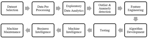
Data-driven models require data generated by sensors that measure physical characteristics such as pressure, temperature, and flow rate. The current research makes use of the publicly accessible NASA PCOE dataset, which contains the operational history of 100 aircraft engines, as well as readings from 21 sensors such as pressure, temperature, and flow rate. The dataset comprises around 100 cycles for each engine. The data set contains the averaged parameters of the model for each cycle of operation and are typically recorded until the engine reaches run-to-failure, which is the end of the engine’s life. Usually, the standard enterprise database collection system collects the sensor data and store the data in frameworks like SAP. The data is converted from the regular comma separated values (CSV) format to the panda framework using the panda analysis package in Python to facilitate data analysis on specific modules and to understand data's nomenclature such as missing values, null entries, and so on. Figure 2 illustrates the overall data analysis approach adapted in the current research.
The framework begins with a dataset that is typically available in enterprise databases such as SQL and Oracle. The data collection is first preprocessed to remove null values, NA values, and empty cells to ensure that the model runs smoothly and doesn’t interfere with model processing. The Key Performance Indicators are determined by exploratory data analysis. A suitable method is used to identify and remove outliers and anomalies. Feature engineering is used to extract few features from the available large number of sensors. An ensemble algorithm with various regression and neural network models including the machine and business intelligence are deployed [22]. This generates quick alarms and plans the operations and maintenance of any complex system automatically. A fraction of the training data captured from the engine is shown in the following Table 1.
Here, Id: Identity number of the engine
Cycle: Count of the cycle of operation
Setting 1: Operation mode 1
Setting 2: Operation mode 2
Setting 3: Operation mode 3
S1-21: Sensor Values captured for 21 sensors of various physical parameters.
The fundamental statistical distribution of sensor values is first understood through data analysis. The maximum, minimum, range, mean, and standard deviation were calculated for all variables and are shown in Table 2.
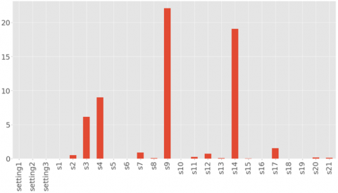
The standard deviation of any variable reflects the likelihood that the sensor will contribute significantly to the prediction of the target variable. For instance, Figure 3 demonstrates that sensor 9 has the highest standard deviation in comparison to all other sensors. Additionally, standard deviation plays a crucial role in discovering anomalies and detecting outliers.
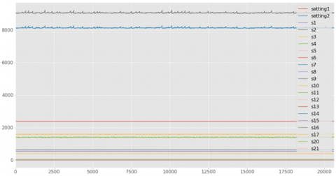
Multiple variables are included in the data, and the relationship between them is the fundamental phenomenon that must be considered while developing a predictive model. As a result, a pandas correlogram is used to find correlation between sensors. The correlation matrix depicts how each parameter is interdependent on the others. As a consequence, a greater correlation 1 indicates that they are more dependent on one another. The association between sensors and non-zero standard deviations, for example, is depicted in Figure 4.
Figure 2. Analytics framework for sensor data analysis
Table 1. Dataset of aircraft sensor data
Table 2. Key statistics of the variables
|
Id |
Cycle |
setting1 |
setting3 |
s1 |
s2 |
s3 |
s4 |
|
|
Count |
20631 |
20631 |
20631 |
20631 |
20631 |
20631 |
20631 |
20631 |
|
Mean |
51.506 |
108.807 |
-8.9E-06 |
100 |
518.67 |
642.68 |
1590.523 |
1408.93 |
|
Std |
29.227 |
68.8809 |
0.00218 |
0 |
6.54E-11 |
0.5000 |
6.13115 |
9.00060 |
|
Min |
1 |
1 |
-0.008 |
100 |
518.67 |
641.21 |
1571.04 |
1382.25 |
|
25% |
26 |
52 |
-0.0015 |
100 |
518.67 |
642.325 |
1586.26 |
1402.36 |
|
50% |
52 |
104 |
0 |
100 |
518.67 |
642.64 |
1590.1 |
1408.04 |
|
75% |
77 |
156 |
0.0015 |
100 |
518.67 |
643 |
1594.38 |
1414.55 |
|
Max |
100 |
362 |
0.0087 |
100 |
518.67 |
644.53 |
1616.91 |
1441.49 |
Figure 3. Standard deviation of all variables (Zero &Non-Zero)
Figure 4. Dataset with non-zero standard deviation
As described in Figure 4, out of all the 21 variables only variables which are having Non-zero standard deviation are considered for feature selection. Zero Standard deviation variables remain constant throughout the operation.
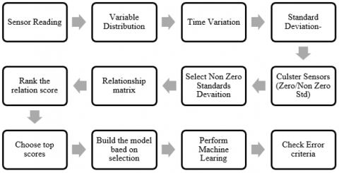
In this proposed methodology, a novel solution as illustrated in Figure 5 is presented to perform feature engineering, find the critical sensors and the relationship among them using the following ensemble of algorithms. Initially, sensor readings are supplied to the framework in a suitable data format. Then the distribution of all variables is studied using statistical tools, and statistical properties are evaluated. A time or cyclic variation of the data is derived using the difference of consecutive data points. The standard deviation of the whole dataset is computed initially, and the same is classified into zero or non-zeros clusters. All non-zero standard deviation variables are grouped to be eligible for participation in further computation. For a non-zero group of sensors, a relationship matrix is formed. The computed relationship matrix is based on the Vector Auto Regression approach. Vector Auto Regression approach is a multi-variable probabilistic model that will give the probabilistic relationships among two variables through the impulse response function. VAR computation methodology is a standard library. Hence the explanation of the same is beyond the scope of the current paper. VAR considers the Lead /Lag relationship and influence probability between two variables to build the relationship matrix. From the relationship table, a ranking algorithm is used to find the variables with higher relation. These chosen sets of variables will be further used for developing machine learning algorithms. An error criterion like Root Mean Square Error (RMSE) is used to cross-check the model’s accuracy for a chosen set of sensor values.
4.1 Response relation algorithm
Input: Multivariate Time Series Data.
Output: Significant features to be used in prediction.
Step 1: Consider time series data S=[s1,s2,s3…sn]
For each Si in S
Calculate Std(Si)
If Std(Si==0)
zs=append.Si //append to Zero Cluster of variables
else
nzs=append.S //append to Nonzero Cluster of Variables
Step 2: For each Si in nzs
res= ADFtest(Si)
If res is stationary
goto step3
else
apply transformations and goto step 2
Step 3: Granger casuality test (nzs)
For each Si in nzs
For each Sj in nzs
grangercasuality(Si,Sj)
If (P-Value<=0.05) && (Fvalue>Fmean)
Add(Si.Sj) to selected variables
Step 4: For each Si in selected variables list
sumlag(Si) //find the sum of all lags
Step 5: Rank them based on the highest value
Step 6: Choose the top most ranked variables to participate in the prediction of RUL.
Figure 5. Response Relation methodology
Given a variable, several statistical tools and machine learning models are used to forecast its future value. These are models capable of forecasting for a single or numerous variables. Typically, models are constructed using simple linear approaches or sophisticated neural networks and begin with a fundamental mathematical relationship between one or more independent variables and the dependent variable. Linear Regression is a machine learning approach that uses supervised learning to perform regression tasks. Regression modelling is used to create a target prediction value based on independent variables. It is mostly used to establish relationships between variables and to forecast their future values. The regression models vary in terms of the number of independent variables and the relationship between the independent and dependent variables. Linear regression models are more appropriate when the parameters are linearly dependent on one another. The current research is aimed at precisely calculating the remaining time to failure for all engines. As a result, the dependent variable is defined as the time to failure (TTF). A linear regression model is a critical component of any predictive study since it provides the initial estimate.
Table 3 indicates the statistical relationship value among all the variables after applying the selection ranking criteria as 0.05. This ranking can be chosen based on the dataset and domain expertise.
Table 3. Relationship table after selection
|
setting1 |
s4 |
s6 |
s7 |
s13 |
s14 |
s15 |
s17 |
s20 |
s21 |
ttf |
|
|
Variable |
0.35 |
0.00 |
0.00 |
0.00 |
0.00 |
0.00 |
0.00 |
0.00 |
0.00 |
0.00 |
0.00 |
|
setting2 |
0.03 |
0.03 |
0.60 |
0.98 |
0.37 |
0.23 |
0.31 |
0.68 |
0.42 |
0.09 |
0.05 |
|
s4 |
0.50 |
0.01 |
0.02 |
0.02 |
0.03 |
0.56 |
0.00 |
0.04 |
0.14 |
0.12 |
0.02 |
|
s8 |
0.45 |
0.00 |
0.90 |
0.00 |
0.00 |
0.00 |
0.00 |
0.05 |
0.14 |
0.06 |
0.00 |
|
s20 |
0.50 |
0.01 |
0.57 |
0.01 |
0.09 |
0.62 |
0.00 |
0.01 |
0.07 |
0.00 |
0.05 |
|
s6 |
0.81 |
0.21 |
0.04 |
0.62 |
0.01 |
0.75 |
0.05 |
0.30 |
0.35 |
0.62 |
0.02 |
|
s13 |
0.75 |
0.70 |
0.03 |
0.01 |
0.00 |
0.00 |
0.63 |
0.06 |
0.14 |
0.01 |
0.05 |
|
s11 |
0.80 |
0.00 |
0.71 |
0.00 |
0.00 |
0.57 |
0.00 |
0.00 |
0.00 |
0.01 |
0.04 |
From the above table, seven sensors are selected before feeding the machine learning prediction algorithm. These sensors are namely setting2, s4, s6, s8, s11, s13, and s20.
Once the selection of variables based on the response relation method is made, these variables are chosen to participate in machine learning prediction. In the current experimental study, seven variables are selected from 24 parameters of the aircraft system. To demonstrate the comparison of the proposed method against all variable method predictions of RUL, Binary, and Multi-Class classification is conducted separately for both approaches. Finally, a comparative analysis is performed on the results. The current work employs a combination of regression techniques such as Linear, RIDGE, Random Forest, LASSO, Polynomial Regression, Decision Tree, SVC and MLP Classifier.
5.1 Prediction of RUL (Remaining Useful Life)
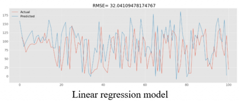
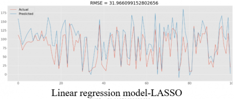
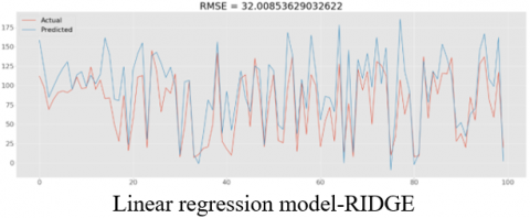
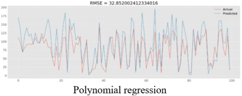
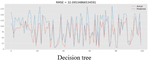
The graphs in Figure 6 represent the sample predicted and actual values using various models for all variable scenarios. In addition, a similar prediction is performed using Response Relation (RR) approach.
The key requirement of a predictive maintenance algorithm is to predict the time to failure. Different Models are investigated for time to failure, with the SVC model predicting the time to failure prior to 25 cycles with an RMSE of 25. The same is computed for the response relation method, and the results are presented in Table 4.
Figure 6. RMSE comparison of actual & predicted values for various models with sensors
As described in Figure 6 RMSE values range from 25 to 32 cycles. Out of all the algorithms SVC gave minimum RMSE.
Table 4. RUL prediction using different models
|
|
RMSE-All |
R2-All |
MAE-All |
RMSE-RR |
R2-RR |
MAE-RR |
|
Linear Regression Model |
32.041 |
0.4054 |
25.5917 |
34.459 |
0.3123 |
26.830 |
|
Linear –LASSO |
31.966 |
0.40827 |
25.5518 |
34.33 |
0.3171 |
26.730 |
|
Linear –RIDGE |
32.008 |
25.5702 |
0.40670 |
34.42 |
0.3137 |
26.795 |
|
Polynomial Regression |
32.852 |
0.37502 |
25.1062 |
33.81 |
0.3379 |
25.887 |
|
Random Forest |
28.899 |
0.51636 |
23.3600 |
32.58 |
0.3851 |
24.989 |
|
Decision Tree |
40.917 |
0.03047 |
26.3400 |
34.71 |
0.3020 |
26.736 |
|
MLP Classifier |
45.4794 |
0.1977 |
36.4800 |
38.62 |
0.1787 |
34.486 |
|
SVC |
25.50235 |
0.62338 |
19.6900 |
24.43 |
0.6123 |
18.583 |
RMSE-All: Root Mean Square Error considering all variables in the dataset.
R2-All: R squared error considering all the variables in the dataset.
MAE-All: Mean Absolute error considering all the variables in the dataset.
RMSE-RR: Root Mean Square Error with significant variables obtained from Relative Response.
R2-RR: R squared error with significant variables obtained from Relative Response.
MAE-RR: Mean Absolute error with significant variables obtained from Relative Response.
5.2 Binary classification
Any industrial IoT system must incorporate decision-making capabilities. The algorithm's output must be expressed in terms of the profits that the business can reap. Based on the projected costs and profits for maintenance and operation in the current analysis, the KNN model provided the largest commercial advantage. The results of Binary Classification using all the variables in the dataset and comparison for binary classification using only the significant features obtained from relative response method are presented in Table 5 and Table 6, respectively. We compared the different models based on True and False Positive Rates (TPR, FPR). Theoretical basis for the response relationship methodology which is basis for these experiments is presented in section 4.1. The Mathematical procedure for each algorithm is available in open literature.
Here, TP-True Positive FP-False Positive
TN-True Negative FN-False Negative
TPR-True positive Ratio FPR-False Positive Ratio
Table 5. Comparison of binary classification with all the variables in the dataset
|
Model |
TP |
FP |
TN |
FN |
TPR |
FPR |
|
|
1 |
KNN |
25 |
0 |
69 |
6 |
0.806 |
0 |
|
2 |
Random Forest |
25 |
0 |
67 |
8 |
0.757 |
0 |
|
3 |
Logistic Regression |
22 |
3 |
73 |
2 |
0.916 |
0.6 |
|
4 |
SVC Linear |
22 |
3 |
70 |
5 |
0.814 |
0.37 |
|
5 |
Gaussian NB |
21 |
4 |
67 |
8 |
0.724 |
0.33 |
|
6 |
SVC |
18 |
7 |
62 |
13 |
0.580 |
0.35 |
Table 6. Comparison of binary classification with the significant variables from response relation
|
Model |
TP |
FP |
TN |
FN |
TPR |
FPR |
|
|
1 |
Random Forest |
25 |
1 |
70 |
4 |
0.8631 |
0.085 |
|
2 |
KNN |
27 |
1 |
69 |
3 |
0.96 |
0.073 |
|
3 |
Logistic Regression |
25 |
2 |
69 |
5 |
0.917 |
0.073 |
|
4 |
Gaussian NB |
23 |
2 |
68 |
4 |
0.8558 |
0.084 |
|
5 |
SVC Linear |
24 |
3 |
68 |
5 |
0.8793 |
0.089 |
|
6 |
SVC |
24 |
1 |
70 |
5 |
0.8796 |
0.091 |
5.3 Multiclass classification
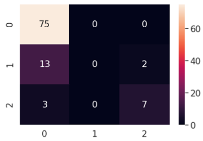
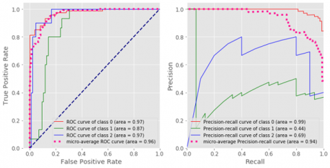
A multi-class classification is a valuable tool for decision-making in industrial IoT applications. Typically, the operator is interested in knowing the time in which an engine will fail. In current research multi-class label is generated for the RUL cycle of 30 cycles. Figures 7 to 18 show the multi-class Classification matrix along with respective multi-class classification Statistics for Logistic Regression, Gaussian NB, SVC, KNN MLP and Decision Tree. Similar Computations are performed for the proposed response relation method, and finally, a comparison of both is made as shown in Tables 7 and 8.
In current study classification results with multiple algorithm experiments to prove that response relationship method provides acceptable results.
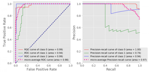
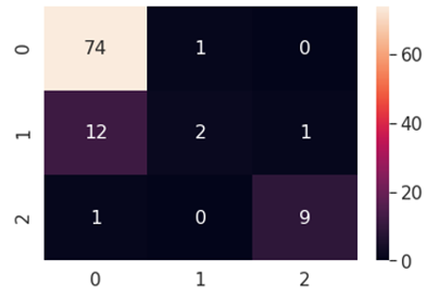
Figure 7. Multi-class confusion matrix –SVC
Figure 8. Multi-class classification statistics- SVC
Support Vector Classifier Linear model: The support vector classifier (SVC) is a statistical technique that is used to determine the linear relationship between two continuous variables. SVC is memory efficient, which means it takes a relatively lower calculation resource to train the model, giving enormous computational advantages.
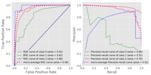
Logistic Regression Model: Logistic Regression is a machine learning approach for binary classification in which the dependent variable is a binary variable. It forecasts the likelihood of occurrence of a categorical dependent variable with data coded as 1 (yes, success, etc.) or 0. (no, failure, etc.).
Figure 9. Multi-class confusion matrix- logistic regression
Figure 10. Multi-class classification statistics- logistic regression
Figure 11. Multi-class confusion matrix – KNN model
Figure 12. Multi-class classification statistics – KNN model
Figure 13. Multiclass confusion matrix –GB model
Figure 14. Multi-class classification statistics –GB model
Figure 15. Multi-class confusion matrix –MLP model
Figure 16. Multi-class classification statistics –MLP model
K-Nearest Neighbors model: K-Nearest Neighbors (KNN) is a standard machine learning approach that is a non-parametric, lazy learning algorithm that makes no assumptions about the data it is learning. The numerical values are chosen based on their proximity to other data points, regardless of what feature they represent. Additionally, because this is a lazy learning method, there is minimal or no training step.
Gaussian Naive Bayes Model: Gaussian Naive Bayes is a variation of Naive Bayes that is based on the Gaussian normal distribution and is capable of handling continuous data. The model fitting is by calculating the mean and standard deviation of the points within each label, that is required to construct a distribution of this type. It is assumed that the data is characterised by a Gaussian distribution with no covariance between dimensions (independent dimensions).
Multi Layer Perceptron model: A Multi Layer Perceptron (MLP) can be thought of as a logistic regression classifier that uses a learned nonlinear transformation to alter the input. By projecting the input data to space, this transformation renders the data linearly separable. A hidden layer is a term which refers to this intermediary layer. MLPs can be used as a universal approximator with just one hidden layer.
Decision Tree model: A decision tree is both a Classification and Regression approach, typically used to solve Classification problems. It is a technique for Supervised Learning using a tree structure in which the internal nodes represent the features of a dataset, the branches represent the decision rules, and each leaf node represents the output. A Decision tree's two nodes symbolize the Decision Node and the Leaf Node. Decision nodes are used to make decisions and have numerous branches, whereas Leaf nodes represent the result of such decisions and contain no additional branches.
Figure 17. Multi-class classification confusion matrix-decision tree
Figure 18. Multi-class classification statistics-decision tree
Table 7. Comparison of multi classification using all variables of the dataset
|
Accuracy |
F1 |
Precision |
Recall |
ROC AUC |
|
|
Logistic Regression |
0.78 |
0.53 |
0.55 |
0.52 |
0.93 |
|
Decision Tree |
0.78 |
0.54 |
0.58 |
0.52 |
0.93 |
|
Random Forest |
0.79 |
0.56 |
0.56 |
0.55 |
0.94 |
|
SVC Linear |
0.79 |
0.53 |
0.62 |
0.50 |
0.91 |
|
KNN |
0.83 |
0.63 |
0.72 |
0.58 |
0.93 |
|
Gaussian NB |
0.68 |
0.68 |
0.60 |
0.87 |
0.91 |
|
Neural Net MLP |
0.83 |
0.64 |
0.75 |
0.60 |
0.94 |
Table 8. Comparison of multi classification using significant variables from relative response method
|
Accuracy |
F1 |
Precision |
Recall |
ROC AUC |
|
|
Logistic Regression |
0.81 |
0.56 |
0.55 |
0.56 |
0.95 |
|
Decision Tree |
0.84 |
0.68 |
0.82 |
0.67 |
0.91 |
|
Random Forest |
0.82 |
0.61 |
0.78 |
0.57 |
0.96 |
|
SVC Linear |
0.60 |
0.46 |
0.60 |
0.38 |
0.93 |
|
KNN |
0.83 |
0.64 |
0.80 |
0.60 |
0.90 |
|
Gaussian GB |
0.74 |
0.76 |
0.66 |
0.98 |
0.95 |
|
Neural Net MLP |
0.84 |
0.75 |
0.85 |
0.69 |
0.95 |
Based on all the Models MLP Model is chosen as the most suitable model for the current dataset. MLP model gave an accuracy of 84% and AUC of 95%. Multi Layer Perception Model proves better accuracy due to multiple layers of Neural Networks used in the architecture. Working Details of MLP Algorithm is available in open literature. Based on the two metrics of accuracy and AUC, multi-class classification is selected as the most suitable model for this dataset. The results from all variable methods and the Relative Response Method are in good agreement, as depicted in Figure 19 and Figure 20. Furthermore, the proposed Relative Response Method matches very well with the results of all variable method. The Primary reason for effectiveness of response relationship method lies in deriving the relationship variables that are responsible for the outcome variable, in this case RUL. The current procedure eliminated non response variables, hence better accuracy.
Figure 19. Comparing binary classification results
Figure 20. Comparing multi classification results
Industrial IoT is an emerging technology that can significantly assist in enhancing machine’s secure and intelligent operation. A practical application of such technology integrates machine learning models facilitating the business benefits. An integrated framework is developed for Industrial IoT with feature selection as one of the critical aspects of IoT system development and application. Feature elimination ranges from using a standard deviation-based approach to complex energy-based indicators unlike Physics-driven models which rely on the interrelation of variables that are participating in a phenomenon. In data-driven approach, the relationship needs to be established using interrelation among sensor variables in response and relation. In the present study, the approach is to choose few critical sensors from all the available sensors combined with machine learning models like KNN, Decision Tree, Logistic Regression, and SVC. Relation Response method applied to both Binary and Multi-Classification methods indicate that Relative Response method matches well with all variable methods. Further, this method when applied to Binary and Multi-class classification proved to be very effective.
|
IoT |
Internet of Things |
|
PHM |
Prognostics and Health Management |
|
RUL |
Remaining Useful Life |
|
C-MAPSS |
Commercial Modular Aero-Propulsion System Simulation |
|
MLP |
Multilayer Perceptron |
|
KNN |
K-Nearest Neighbors |
|
LASSO |
Least Absolute Shrinkage and Selection Operation |
|
SVC |
Support Vector Classifier |
|
RMSE |
Root Mean Square Error |
|
MSE |
Mean Square Error |
|
RMS prop |
Root Mean Square propagation |
|
TPR |
True Positive Ratio |
|
FPR |
False positive Ratio |
|
TP |
True Positive |
|
FP |
False Positive |
|
TN |
True Negative |
|
FN |
False Negative |
|
AUC ROC |
Area Under Receiver Operating Characteristics Curve |
[1] Yan, K., Zhang, D. (2015). Feature selection and analysis on correlated gas sensor data with recursive feature elimination. Sensors and Actuators B: Chemical, 212: 353-363. https://doi.org/10.1016/j.snb.2015.02.025
[2] Day, P., Iannucci, S., Banicescu, I. (2020). Autonomic feature selection using computational intelligence. Future Generation Computer Systems, 111: 68-81. https://doi.org/10.1016/j.future.2020.04.015
[3] Su, S., Sun, Y., Gao, X., Qiu, J., Tian, Z. (2019). A correlation-change based feature selection method for IoT equipment anomaly detection. Applied Sciences, 9(3): 437. https://doi.org/10.3390/app9030437
[4] Mosallam, A., Medjaher, K., Zerhouni, N. (2013). Bayesian approach for remaining useful life prediction. Chemical Engineering Transactions, 33: 139-144. https://doi.org/10.3303/CET1333024
[5] Li, X., Ding, Q., Sun, J.Q. (2018). Remaining useful life estimation in prognostics using deep convolution neural networks. Reliability Engineering & System Safety, 172: 1-11. https://doi.org/10.1016/j.ress.2017.11.021
[6] Yu, T., Wang, X., Shami, A. (2017). Recursive principal component analysis-based data outlier detection and sensor data aggregation in IoT systems. IEEE Internet of Things Journal, 4(6): 2207-2216. https://doi.org/10.1109/JIOT.2017.2756025
[7] Hromic, H., Le Phuoc, D., Serrano, M., Antonić, A., Žarko, I.P., Hayes, C., Decker, S. (2015). Real time analysis of sensor data for the Internet of Things by means of clustering and event processing. In 2015 IEEE International Conference on Communications (ICC), pp. 685-691. https://doi.org/10.1109/ICC.2015.7248401
[8] Ren, L., Cui, J., Sun, Y., Cheng, X. (2017). Multi-bearing remaining useful life collaborative prediction: A deep learning approach. Journal of Manufacturing Systems, 43: 248-256. https://doi.org/10.1016/j.jmsy.2017.02.013
[9] Le Son, K., Fouladirad, M., Barros, A., Levrat, E., Iung, B. (2013). Remaining useful life estimation based on stochastic deterioration models: A comparative study. Reliability Engineering & System Safety, 112: 165-175. https://doi.org/10.1016/j.ress.2012.11.022
[10] Liao, H., Zhao, W., Guo, H. (2006). Predicting remaining useful life of an individual unit using proportional hazards model and logistic regression model. In RAMS'06. Annual Reliability and Maintainability Symposium, pp. 127-132. https://doi.org/10.1109/RAMS.2006.1677362
[11] Liu, L., Guo, Q., Liu, D., Peng, Y. (2019). Data-driven remaining useful life prediction considering sensor anomaly detection and data recovery. IEEE Access, 7: 58336-58345. https://doi.org/10.1109/ACCESS.2019.2914236
[12] Medjaher, K., Tobon-Mejia, D.A., Zerhouni, N. (2012). Remaining useful life estimation of critical components with application to bearings. IEEE Transactions on Reliability, 61(2): 292-302. https://doi.org/10.1109/TR.2012.2194175
[13] Zhang, Z., Si, X., Hu, C., Lei, Y. (2018). Degradation data analysis and remaining useful life estimation: A review on Wiener-process-based methods. European Journal of Operational Research, 271(3): 775-796. https://doi.org/10.1016/j.ejor.2018.02.033
[14] Wang, Q., Zheng, S., Farahat, A., Serita, S., Gupta, C. (2019). Remaining useful life estimation using functional data analysis. In 2019 IEEE International Conference on Prognostics and Health Management (ICPHM), pp. 1-8. https://doi.org/10.1109/ICPHM.2019.8819420
[15] Wang, T., Yu, J., Siegel, D., Lee, J. (2008). A similarity-based prognostics approach for remaining useful life estimation of engineered systems. In 2008 International Conference on Prognostics and Health Management, pp. 1-6. https://doi.org/10.1109/PHM.2008.4711421
[16] Loutas, T.H., Roulias, D., Georgoulas, G. (2013). Remaining useful life estimation in rolling bearings utilizing data-driven probabilistic e-support vectors regression. IEEE Transactions on Reliability, 62(4): 821-832. https://doi.org/10.1109/TR.2013.2285318
[17] Hoi, S.C., Wang, J., Zhao, P., Jin, R. (2012). Online feature selection for mining big data. In Proceedings of the 1st International Workshop on Big Data, Streams and Heterogeneous Source Mining: Algorithms, Systems, Programming Models and Applications, pp. 93-100. https://doi.org/10.1145/2351316.2351329
[18] Wang, J., Zhao, P., Hoi, S.C., Jin, R. (2013). Online feature selection and its applications. IEEE Transactions on Knowledge and Data Engineering, 26(3): 698-710. https://doi.org/10.1109/TKDE.2013.32
[19] Wu, Y., Hoi, S.C., Mei, T., Yu, N. (2017). Large-scale online feature selection for ultra-high dimensional sparse data. ACM Transactions on Knowledge Discovery from Data (TKDD), 11(4): 1-22. https://doi.org/10.1145/3070646
[20] Perkins, S., Theiler, J. (2003). Online feature selection using grafting. In Proceedings of the 20th International Conference on Machine Learning (ICML-03), pp. 592-599.
[21] Zhou, J., Foster, D.P., Stine, R.A., Ungar, L.H. (2006). Streamwise feature selection. Journal of Machine Learning Research, 7: 1861-1885.
[22] Kalyani, S., Venkat Rao, K., Mary Sowjanya, A. (2020). Integrated intelligent framework for sensor data analysis. World Academics Journal of Engineering Sciences, 7(3): 52-59.
[23] Yu, K., Wu, X., Ding, W., Pei, J. (2016). Scalable and accurate online feature selection for big data. ACM Transactions on Knowledge Discovery from Data (TKDD), 11(2): 1-39. https://doi.org/10.1145/2976744
[24] Minor, B.D., Doppa, J.R., Cook, D.J. (2017). Learning activity predictors from sensor data: Algorithms, evaluation, and applications. IEEE Transactions on Knowledge and Data Engineering, 29(12): 2744-2757. https://doi.org/10.1109/TKDE.2017.2750669
[25] Liu, L., Wang, S., Liu, D., Peng, Y. (2017). Quantitative selection of sensor data based on improved permutation entropy for system remaining useful life prediction. Microelectronics Reliability, 75: 264-270. https://doi.org/10.1016/j.microrel.2017.03.008
[26] Mosallam, A., Medjaher, K., Zerhouni, N. (2016). Data-driven prognostic method based on Bayesian approaches for direct remaining useful life prediction. Journal of Intelligent Manufacturing, 27(5): 1037-1048. https://doi.org/10.1007/s10845-014-0933-4
[27] Djeziri, M.A., Benmoussa, S., Sanchez, R. (2018). A hybrid method for remaining useful life prediction in wind turbine systems. Renewable Energy, 116: 173-187. https://doi.org/10.1016/j.renene.2017.05.020
[28] Si, X.S., Wang, W., Hu, C.H., Zhou, D.H. (2011). Remaining useful life estimation–a review on the statistical data-driven approaches. European Journal of Operational Research, 213(1): 1-14. https://doi.org/10.1016/j.ejor.2010.11.018
[29] Zhang, C., Lim, P., Qin, A.K., Tan, K.C. (2016). Multiobjective deep belief networks ensemble for remaining useful life estimation in prognostics. IEEE Transactions on Neural Networks and Learning Systems, 28(10): 2306-2318. https://doi.org/10.1109/TNNLS.2016.2582798
[30] Wu, Y., Hoi, S.C., Mei, T., Yu, N. (2017). Large-scale online feature selection for ultra-high dimensional sparse data. ACM Transactions on Knowledge Discovery from Data (TKDD), 11(4): 1-22. https://doi.org/10.1145/3070646
[31] Katukam, R., Behera, P. (2014). Engineering optimization using artificial neural network. International Journal of Innovations in Engineering & Technology (IJIET), 4(3): 63-72.
[32] Moraru, A., Pesko, M., Porcius, M., Fortuna, C., Mladenic, D. (2010). Using machine learning on sensor data. Journal of Computing and Information Technology, 18(4): 341-347. https://doi.org/10.2498/cit.1001913
[33] Taha, H.A., Sakr, A.H., Yacout, S. (2019). Aircraft engine remaining useful life prediction framework for Industry 4.0. In 4th North America Conference on Industrial Engineering and Operations Management, Toronto, Canada.
[34] Okoh, C., Roy, R., Mehnen, J., Redding, L. (2014). Overview of remaining useful life prediction techniques in through-life engineering services. Procedia Cirp, 16: 158-163. https://doi.org/10.1016/j.procir.2014.02.006