Nicoletta Lotrecchiano | Daniele Sofia | Aristide Giuliano* | Diego Barletta | Massimo Poletto
© 2020 IIETA. This article is published by IIETA and is licensed under the CC BY 4.0 license (http://creativecommons.org/licenses/by/4.0/).
OPEN ACCESS
A deterministic approach was used in this work to assess the PM2.5 pollutant dispersion in the air during a fire event. The pollution data were recorded with high time resolution by a monitoring station located 4 km South-West from the fire. The pollutant emission due to the fire was described as an equivalent stack having the height of the observed cloud of generated smoke. The pollutant dispersion was modelled by means of a Gaussian plume dispersion model. To this purpose, the unknown equivalent emission mass flow rate at the stack in the model was found out using the available experimental data of PM2.5 measured on the ground far away, considering the changing of the air stability between nighttime and daytime and the variable wind direction. Model results highlighted that the predicted maximum pollutant concentration was larger of an order of magnitude than the data value recorded at the monitoring station and exceeded the law limit value. A sensitivity analysis on the wind speed and the atmospheric stability conditions was performed as well to identify the worst case scenarios in case of a fire event. The main conclusion is that a dense network of measurement stations with high time resolution is necessary to properly monitor an area or to provide validation data for any predicting dispersion model in case of a pollutant release.
fire, air quality, Gaussian Plume, dispersion model, monitoring, mapping, pollution, 2D-modeling
Fires are accidental events determined by different causes, produced by natural events, such as accumulation of gases due to the decomposition of organic matters exposed to high temperatures, lightning, etc. or by human actions for unexpected, legitimate or illicit reasons.
Gases, smoke and vapors that develop during the non-controlled combustion occurring in a fire can also be responsible for significant damages to both humans and the environment. Smoke is perhaps the most visible part of the product of a fire. It can be made of very fine solid particles suspended in the gas phase, as well as of condensed vapors. Gases produced in a fire are able to maintain their state also when cooling at ambient temperature. Vapors leaving the fire can become solid or liquid at ambient temperature and, when they move away from the flame, may condense and adhere to cold surfaces or form particles (aerosols) that remain suspended and moved by wind. Gases and vapors produced in a fire and coming in contact with humans can cause discomfort to breathe, irritation, interact with skin or internal tissues, such as nasal mucous membranes, lungs, organs, and internal organs, producing dangerous effects due to long exposures [1]. Smoke, gases and vapors developed in a fire in an industrial site may be more or less dangerous in relation to the kind of materials involved, especially if they include potential sources of toxic compounds such as it happens for paints and polymeric materials. When such compounds are released in a fire, they can spread in the air to the ground and to the waterways of the areas surrounding the fire. The main gas and vapor compounds produced as a result of a fire which are responsible of pathological effects are: carbon monoxide (CO); carbon dioxide (CO2); hydrogen cyanide (HCN); hydrochloric acid (HCl); nitrogen oxides (nitrous oxide - N2O -, nitric - NO -, and two forms of dioxide - NO2 and N2O4 -); dioxins and furans. For most of these compounds both the amount released in a fire and the spatial extent of the contamination produced can be evaluated by using different models which make use of the composition of the burnt material, the fire conditions and the transport and dispersion in the air. For these compounds the toxic effect, mainly linked to the presence of the cloud released by the fire, often ceases with the dissolution of the cloud. However, dioxins can deposit on the plants, on the soil, in the water courses and can be ingested by the fauna that populates these areas, accumulating in their organisms [2]. Such situation has determined the need to study the possible mechanisms of dioxin formation in order to assess the effects of contamination. The type of smoke produced in a fire depends on the type and on the state of aggregation of the fire fuel, of the type of ignition and the mode of combustion that develops in relation to the ventilation conditions of the fire itself. The state of air quality in a town, especially after important events such as fires, is the result of a complex combination of a multitude of physical and chemical transformations. Physical transformations are mostly related to transport processes determined by air motion, which tends to disperse, convey and deposit the chemical species directly emitted by pollution sources, the so called primary pollutants. Chemical-physical transformations, instead, can be responsible of the formation of new polluting species, called secondary pollutants. The dispersion of pollutants, caused by air instability (vertical dispersion) and transport of air masses (horizontal convection and dispersion), as well as their chemical transformation or deposits are strictly dependent on the dynamic behavior of the lower layers of the atmosphere. Therefore, in order to draw a clear picture of the extent of the local pollution related to a fire and its impact in the surrounding areas, it is important to know both the point of origin of a fire and the environmental parameters which allow to integrate the space and time distribution of the pollutants.
Due to the accidental nature of a fire, environmental monitoring related to a fire cannot be scheduled. Furthermore, given the variety of substances that can be potentially burned in a fire and the different territorial characteristics of the areas that may be affected, it is not possible to define in advance a standardized monitoring protocol to be applied in case of fire. Even if it is always possible to identify some recurring phases of the monitoring activity connected to the evolution of the fire, the measurement campaign will still have to be designed based on the event, the materials and substances affected by the fire, the place and its environmental characteristics and sensitivity. In order to have a complete view of the environmental situation, it is recommended to install in urban areas air quality monitoring networks, which, beside fixed monitoring stations [3], could also include mobile monitoring stations of the new generations, like Real-time on-road monitoring stations [4]. Such kind of network ensures high space-time resolution of air quality measurements, which can be used not only to define the levels of pollution but also to trace back the pollution and define its sources [5]. Furthermore, in case of environmental accidents such as fires, the above-mentioned networks allow to instantaneously evaluate the effects of the event on the air quality and help the authorities and the citizens to better understand the actual environmental situation. In case of everyday air monitoring, the immediate knowledge of pollution levels and their origins can lead to the definition of the most appropriate strategies for their reduction, with reference to mitigation strategies that involve the decarbonization of the energy sources. In fact, these latter combine the reduction of environmental pollution with social benefits [6].
Monitoring of air pollution is also important for purposes related to environmental protection, that is one of the most discussed topics in the recent years. There are many approaches to propose strategies leading to the reduction of pollution. Most of the existing industrial plants are converting to the application of environmental policies that aim at zero emissions and low impacts in general. The industrial plants that use biomass as feedstock should be placed in this perspective. Cherubini [7] proposed the definition of the biorefinery concept intended as the use of most of the potential of biomass by minimizing the wastes and the emissions connected with the production of bioenergy products. One of the most fruitful feedstock is the residual lignocellulosic biomass that, if used, can lead to both the reduction of CO2 emissions and the production of green electricity [8].
Modelling has been often used to evaluate concentration and dispersion process of pollutants in air [9], water [10] and ground [11]. In the modeling field there are various mathematical approaches to describe reality and to define the behavior of solid particles such as particulates, such as discrete element method (DEM) [12]. Dispersion models are useful tools to determine long-term health impacts of the smoke exposures of the local populations [13]. For example, during accidents like fires, the correct modelling of the pollutant distribution in space and time is fundamental for the definition of the human exposure to pollution. In addition to this, the application of dispersion models can have an important role in providing air quality data to promote the social acceptance to reassure of industrial plants with controlled pollutant emissions [14].
As reported by the recent literature survey [15], the dispersion of air pollutants in the atmosphere has been modelled by means of three different approaches: Gaussian dispersion models, Lagrangian models and Eulerian models. Recent studies using the Gaussian dispersion modelling approach were focused on improving the plume rise mechanisms description by means of semi-empirical equations or by more sophisticate models accounting for cloud microphysics and transport [16-18]. Models coupling fire plume dynamics and weather forecast were also developed mainly to forecast the fire plume dispersion [19]. Daly et al. [16] estimated the ground-level exposure in the neighborhood of a fire in a warehouse, by means of two plume dispersion modeling techniques. In particular, in this study the air quality impact of large fires was assessed by assuming the smoke plume as a combination of a hot upper-part staying aloft and a cooler lower-part impacting the ground. Mallia et al. [18] highlighted that emissions injection schemes corresponding to the assumption of both no plume rise and plume-top configurations could not predict satisfactorily the vertical distribution of smoke.
The Lagrangian particle model approach was used by several recent studies [20-22]. Ferrero et al. [21] modelled different schemes of plume rise of smoke emitted from controlled burns without any a priori assumption on the dynamics of the plume or on the atmospheric conditions. Good agreement was obtained by Thakur et al. [22] between model predictions of vertical profiles of CO concentration and satellite observations over the burned areas. Results highlighted a significant increase of CO concentration at altitudes about 3 km height above mean sea level during the fire event. Zhu et al. [20] combined a Lagrangian Flexible Particle dispersion model (FLEXPART) [23] with the Weather Research and Forecasting (WRF) model output [24] to derive the smoke aerosols transported from forest fires. Some recent works on fires [25, 26] used the TAPM model [27] based on fundamental equations of atmospheric flow, thermodynamics, moisture conservation, turbulence and dispersion, combining different sub module approaches (integrated plume rise, Lagrangian particle, building wake, and Eulerian grid modules). A chemical transport model was also combined with a Dispersive Apportionment of Source Impacts (DASI) by Huang et al. [28] to forecast the air quality impact of prescribed fires.
The availability of a model validated with direct experimental measurements of pollutants concentrations is of paramount importance to predict the impact on air quality in the surrounding of prolonged fires and to implement precautionary measures for the population. However, few published studies have validated model predictions with direct measurement of the spatial distribution of pollutant concentration over the time [29].
This work aims at using a modelling approach to derive the dispersion of pollutants emitted by an accidental fire validating the results with measured data regarding air pollution. The Gaussian plume dispersion approach is followed in order to evaluate the mass flow rate of particulate matter originating from a fire by using a limited number of PM2.5 concentration values measured by an air quality monitoring station placed 4 km downwind of the fire starting point.
2.1 Equipment
The data used to feed the modeling procedure are provided by a fixed monitoring station installed in the city of Avellino (Italy). Avellino is a medium sized town located in the Campania region of southern Italy and placed in a wide planar region surrounded by mountains. The city suffers one of the worst air quality of southern Italy due to the intense industrial activity and the local orography that are responsible of atmospheric conditions hindering the dispersion of pollutants. In order to demonstrate the potential of a wider high space and time resolution network, a single monitoring station able of high frequency measurements of the air quality was installed in the city. The station is composed of different air quality sensors and it is based on IoT (Internet of Things) technology. The sensors placed inside the control unit (Figure 1) are able to monitor, among other parameters, concentration of fine particulate solids, the so called PM2.5. In the measurement unit, a weather station can also measure temperature, pressure, relative humidity, wind intensity and direction. All the data are taken every three minutes and are recorded by sending them in real time to a database server. Dedicated software allows to make these data available on the world wide web and to be directly accessed by smartphone.
The measurement system includes an air suction part where specific airflow is conveyed inside the measurement chamber. The measuring chamber is heated and designed to minimize the effects of humidity on the measurement. The sensors inside the system measure the concentrations. In particular, the sensor used to measure the particulate concentrations is based on the principle of laser scattering. The response is processed in the same monitoring station by implementing an algorithm capable of analyzing the sensors' responses in a differential. The data are sent to the central server, which provides for the storage of the information. The sensor arrangement in the measuring device was purposely designed and patented [30] and can be easily modified to be implemented in both a fixed or mobile network. In case of structured network an algorithm for the definition of the optimal sampling positions was implemented [31].
Figure 1. Measuring device
2.2 Modeling
The Gaussian models have been the reference tools for the studies of the pollutant diffusion into the atmosphere and still continue to be valid supports for the assessment of emission scenarios. Their simplicity and immediacy of use and the reliability of the solutions adopted to model the effects of interaction of the plume emitted with the external environment, makes them the most used in the description of pollutant emissions. The emission description within the area studied takes place by associating to each meteorological condition inserted in the Gaussian plume input (values of wind speed and direction, temperature and atmospheric stability) whose shape is modulated by atmospheric conditions. The ease of use of the Gaussian models is linked to the fact that the model requires a type of standard data easily available in the literature both as regards the structural aspect of the emissive sources and the meteorological or geophysical one. The immediacy of use is linked to the rapid response of the model in returning the concentration results. The Gaussian model, implementing an already defined solution of the diffusion equation, does not require its numerical resolution, thus resulting in extremely fast execution even of rather long time intervals.
The simplicity and immediacy of use in addition to the conservative parametric choices used in its calculation algorithms make it a very effective screening tool applicable to the analysis of the diffusion of non-reactive pollutants. Finally, since the quality of the results provided by the Gaussian models is closely linked to compliance with the conditions of applicability and the quality of the meteorological data that are used as input, compliance with these characteristics makes them very effective tools both in the quantitative control phase and as analysis and interpretation tool for the results obtained.
The Gaussian plume dispersion is therefore, the one that better describes the case studied in this work. The fire can be similar to the pollutant emissions from a punctual source.
The application of the model includes some implementation steps that lead to the final results. The definition of the diffusion equation and the boundary conditions are the first implementation step. Then, since the diffusion equation includes dispersion parameters that depends on air stability conditions. So, it is necessary the definition of the wind field characteristics like wind intensity and wind stability class. Then, knowing the height of the stack and the position of the source, the concentration in the point measured, it is possible to obtain the fire mass flow rate.
The Gaussian dispersion model approach was adopted in this study for its simplicity and ease of application.
In order to describe the transport of particulates, which are scarcely affected by chemical transformations in the atmosphere, the advection-diffusion equation describing the mass balance of pollutants in atmosphere does not consider any reaction term [32]:
$\frac{\partial C}{\partial t}+\frac{\partial u C}{\partial x}+\frac{\partial v C}{\partial y}+\frac{\partial w C}{\partial z}=K_{x} \frac{\partial^{2} C}{\partial x^{2}}+K_{y} \frac{\partial^{2} C}{\partial y^{2}}+K_{z} \frac{\partial^{2} C}{\partial z^{2}}$ (1)
where, C is the pollutant concentration, t is time, x is the horizontal spatial coordinate in the wind direction, y is the horizontal spatial coordinate orthogonal to the wind direction, z is the vertical spatial coordinate, u and w are the horizontal and vertical components of the wind velocity, Kx, Ky and Kz are the dispersion coefficients in the three coordinate direction. According to the assumption that advection is the dominant term in the wind direction, it is possible to neglect other terms describing transport in the same direction. Furthermore, it can be assumed that the prevailing wind speed is horizontal, uniform and constant for a sufficiently long timespan, so that the stationary conditions can be applied. Therefore, Eq. (1) reduces to:
$u \frac{\partial C}{\partial x}=K_{y} \frac{\partial^{2} C}{\partial y^{2}}+K_{z} \frac{\partial^{2} C}{\partial z^{2}}$ (2)
Eq. (2) can be solved with the boundary conditions of a continuous point source and the solution is the following [33]:
$C(x, y, z)=\frac{Q}{2 \pi \sigma_{y} \sigma_{z}} \exp \left(-\frac{y^{2}}{2 \sigma_{y}^{2}}\right)\left[\exp \left(-\frac{(z-H)^{2}}{2 \sigma_{z}^{2}}\right)+\exp \left(-\frac{(z+H)^{2}}{2 \sigma_{z}^{2}}\right)\right]$ (3)
where, Q is the pollutant mass flow rate coming out of the source, H is the source height above the ground and the mirror source term (a virtual source located at a height -H ) is introduced to model the worst possible case of air pollution corresponding to a reflection boundary conditions on the ground. σy and σz are defined according the Pasquill-Gifford correlation [34]:
$\sigma_{y}^{2}=\frac{2 K_{y} x}{u} \quad \sigma_{z}^{2}=\frac{2 K_{z} x}{u}$ (4)
i.e. the width and the thickness of the plume described by sy and sz, both increase proportionally with the space time (x⁄u), that is the time taken by the pollutant to reach a certain position x since it was emitted from the source point. The values of the proportionality constants Ky and Kz between the space time and the standard deviation, depend on the tendency of the atmosphere to repress vertical convection, the so-called atmospheric stability. In fact, according to the model, the atmosphere stability affects the parameters Ky and Kz so that unstable conditions have standard deviations that more rapidly increase in the wind direction while stable conditions have standard deviations that less rapidly in the wind direction. Hence, in stable conditions the pollutant may travel longer distances before dispersing. Figure 2 illustrates the situation being modelled.
At a certain downwind distance x, the maximum concentration lies on the plume axis of symmetry and is Cmax:
$C_{\max }(x)=\frac{Q}{2 \pi \sigma_{y} \sigma_{z} u}$ (5)
Therefore, the cloud smoke concentration downwind the stack and at the ground level is calculated as follows:
$c(x, 0,0)=\frac{Q}{\pi \sigma_{y} \sigma_{z} u} \exp \left(-\frac{H^{2}}{2 \sigma_{z}^{2}}\right)$ (6)
The implementation of the Gaussian Plume model was obtained using a MATLAB code derived from the one freely available from the University of Manchester [35]. The code allows to customize several parameters to combine in the model more stack such the one reported above in Eq. (3) by defining the different stack positions on the ground plane, called stack x, stack y, the mass flow rate Q and the height of the stack H.
The values of the vertical stability parameter were set according to the Pasquill atmospheric stability classes [21], which is the most commonly used method of classification of the turbulence in the atmosphere. According to this classification, there are six stability classes named A, B, C, D, E and F with class A being the most unstable or most turbulent class, and class F the most stable or least turbulent class. Each class is defined by meteorological conditions that are the surface wind speed, daytime incoming solar radiation and, night-time cloud cover. Solar radiation increases atmospheric instability through warming of the Earth surface so that warm air finds itself below cooler (and therefore denser) air, a situation that promotes vertical mixing. Clear nights push conditions towards stable as the ground cools faster establishing more stable conditions and inversions. Wind increases vertical mixing, breaking down any type of stratification and pushing the stability class towards neutral (D) [36]. Incoming solar radiation is classified as follows: strong (> 700 W/m2), moderate (350-700 W/m2), slight (< 350 W/m2) [36].
In order to carry out a pollution dispersion analysis, firstly it is necessary to investigate the effects that the assumptions about wind direction have on dispersion of pollutants. Usually, the wind speed and the wind direction would be fed to the model after being determined by either observational data or from weather forecast. Then, it is possible to generate a synthetic dataset by either: (1) having the wind come from a constant direction; (2) having the wind come from a completely random direction and (3) having the wind come from a prevailing direction, with some variation either side.
In the model in this study, a different approach was followed to describe the change of the standard deviations describing the plume thickness and width. Using a common approach, it is:
$\sigma_{y}=a * x^{b}$ (7)
$\sigma_{z}=c * x^{d}+f$ (8)
where, the a, b, c, d, e and f constants depend on the stability class and on the distance, i.e. they may be different for x values smaller or greater than 1 km [37].
2.3 The case study
In this work the migration of pollutants from a real accidental fire occurred in Avellino on 13/09/2019 was studied with the dispersion stack model.
The fire broke out in a company producing plastic containers for automotive batteries. A small part of polypropylene plastic components and many wooden pallets were burned. The starting point of the fire is inside the Avellino industrial development area (F in Figure 2).
Aerosol particles originating from wood burning are predominantly in fine particle mode (PM2.5) [38] while the combustion of PP determines the presence of Pb, Cd and, Zn [39] in the fire smoke. In the model, however, it is assumed that the fire smoke is made of CO2 for 95% in mass and of PM2.5 for the remaining 5% and the corresponding value of the emission factor e is assumed equal to 0.05 [40]. In fact, PM2.5 generally includes all the metals delivered by smoke fires. Concentrations of PM2.5 was measured by a fixed monitoring station (S1 in Figure 2) located at 4 km South-West from the fire.
Figure 2. View of the area around Avellino (Italy) with the fire position (F) and the fixed monitoring stations (S1, A1, A2)
This concentration data was used to evaluate the mass flow of the smoke cloud at its origin in the fire. In Avellino there are also two fixed monitoring stations (A1 and A2 in Figure 2) of the Regional Agency for the Environmental Protection (ARPAC) network providing data of the daily average concentrations. These data were used to verify the model predictions.
Time-series of the PM2.5 concentrations measured by the S1 station are reported in Figure 3. Inspection of the figure reveals a neat increase of PM2.5 after six hours from the fire start (at 1.45 pm), showing a peak of 41 µg/m3. During the night, from 18h to 6h of the next day the PM2.5 concentration fluctuates between 41-12 µg/m3. The instantaneous PM2.5 values measured in the S1 station exceeded the threshold of 25 µg/m3. However, according to Table 1, the regulatory daily average limit, set to the same value by the Italian Law (D.Lgs. 155/2010), was never exceeded.
The PM2.5 concentration measured in real-time by the air quality monitoring station S1 after 12 hours was used as a reference value to infer the fire mass flow rate by applying the Gaussian Plume dispersion model. Subsequently, the best fitting value of the mass flow rate was used as an input to derive ta more complete concentration map at the ground for the Gaussian Plume dispersion model. The resulting model prediction values were compared with the values measured by the monitoring station A1 and A2. Then, to investigate the effect of the wind speed and the wind stability class on the pollutant dispersion, the Gaussian Plume model was applied for different conditions.
In particular, the data used to calculate the average value after 12 hours are provided by the monitoring station every 3 minutes. Data analysis of the distribution of measured values revealed that the interquartile range is 6 μg/m3 (the first quartile is 21 μg/m3, the median is 24 μg/m3, the third quartile is 27 μg/m3). As a result, due to the narrow range and the symmetric distribution during the 12 hours interval, the reference average value for the model was set equal to the median value of 24 μg/m3.
Figure 3. Instantaneous concentrations of PM2.5 measured by S1 and PM2.5. Law limit follows the Italian Law, DLgs. 155/2010
Table 1. Daily average concentrations measured from 13/09/2019 to 15/09/2019 in A1, A2, S1
|
|
PM2.5 daily average concentrations µg / m3 |
||
|
Station\date |
13/09/2019 |
14/09/2019 |
15/09/2019 |
|
Arpac - Sc. V Circolo (A1) |
19.0 |
13.5 |
11 |
|
Arpac - Scuola Alighieri (A2) |
17.6 |
10 |
10.4 |
|
Sense Square (S1) |
23.7 |
14.5 |
5.5 |
The amount of PP stocked was evaluated from the area occupied by the batteries containers that equals to about 2200 m2. Considering a pile height of about 3 m, and the bulk density of the PP around 906 kg/m3 () and a void fraction of 0.9, the total mass of the PP stocked is of 5.0·105 kg. As a result, a total of 5.3·105 kg of fuel burned during the fire for a period of about 12 h, corresponding to an average rate of 12 kg/s. The equivalent stack height of the plume H was estimated equal to 75m, from visual inspection of pictures taken of the smoke column above the fire.
During the fire the wind was blowing from North East and, therefore, moving towards South-West (225°), at 7 m/s. Therefore, in the case study, the position of the air sampling station S1, placed at 4000 m from the fire was on the northern side of the developed smoke plume at about 500 m from the plume axis.
The experimentally measured mean concentration of 24 µg/m3 was used in Eq. (6) to infer the mass flow rate of the pollutant to be used within the model. Considering that the latter value of particulate concentration was mainly measured during the night and that the measured wind speed was about 7 m/s, the D stability class was assumed as a reasonable guess. A first order of magnitude estimate of the flow rate, to be used as a first guess for the subsequent steps was obtained by using Eq. (6). Afterwards, the best fitting mass flow rate value was obtained by minimizing the discrepancy between the measured value at the monitoring station S1. For this purpose, a numerical optimization algorithm was adopted. It was introduced a fixed orthogonal space reference system oriented with the $\xi$ axis in the north direction and the $\eta$ axis in the east direction and with the origin at the fire place. Following this reference system, the coordinates of the S1 monitoring station are (‑ 4000, ‑ 2200).
The mass flow rate producing the best fitting concentration at the monitoring station is 665 g/s. Comparing this value with the burning rate of 12 kg/s above reported, we estimate an emission factor to particulate matter e slightly larger than 5%. This value agrees with literature data [40].
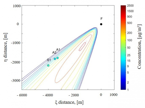
Figure 4 reports the model results in terms of the distribution at the ground level of PM2.5 concentrations. At the monitoring station's position S1, the PM2.5 concentration evaluated by the model is 24.36 µg/m3, with an error of 1.5% respect to the measured value of 24 µg/m3. The maximum of the dust concentration is 950 µg/m3, and it is found at a distance of about 1800 m downwind the fire. Considering the other experimental measurement points (A1 and A2 in Figure 4), it can be seen that the values estimated by the model are in agreement with those measured (average concentration of PM2.5 calculated as for station S1 and described above). In particular, at points A1 and A2, the estimated PM2.5 concentration value differs from the measured one (19.6 µg/m3 for A1 and 14.1 µg/m3 for A2) by 1.5% and 5.2%, respectively. The consistency of the experimental measurements with the values estimated by the model represents a further confirmation of the assumptions' validity.
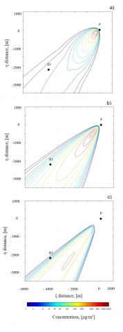
Figure 5 reports the ground level concentrations of PM2.5 estimated with the model in other stability classes. These provide a picture of what might have happened in different times of the day. It appears that, for increasing air stability, the dispersion along the distance decreases, the ground level values tend to increase and the position with the highest pollutant concentration moves away from the fire. The interdependent play between decreased vertical and horizontal dispersion indicated that the conditions corresponding to an intermediate stability class would have provided the highest pollution concentration at the sampling station position.
In order to assess the effect of the fire under different possible meteorological scenarios, by keeping constant the fire rate, the maximum PM2.5 concentrations and their corresponding positions were calculated for all three air stability conditions (A, C, E) and with different wind speeds of 3 and 15 m/s.
Figure 4. PM2.5 concentrations at the ground level according to the Gaussian model for the neutral stability class
Figure 5. PM2.5 plume dispersion in prevailing wind conditions at 7 m/s for: a) very unstable (A), b) slightly unstable (C), c) slightly stable (E) wind field
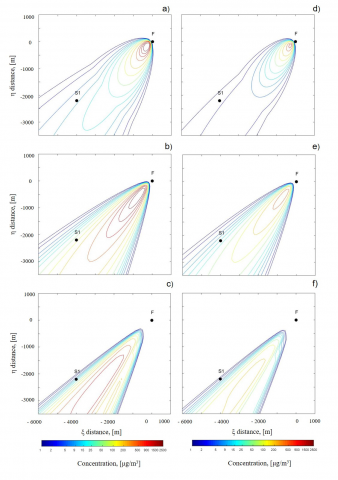
The results of these calculations, together with those of the base case reported above, are summarized in Table 2 and in Figure 6. Inspection of the tables and figures confirms that increasing the wind speed, the dispersion increases, as expected.
At low speeds (3 m/s) (Figure 6a, 6b, 6c), the pollutant dispersion is limited, and the maximum concentration increases with increasing wind stability and is located at progressively greater distances. The pollutant dispersion is favoured by increasing the wind speed (15 m/s) (Figure 6d, 6e, 6f). In fact, with the same wind stability, the maximum concentration decreases. In the model (e.g., see Eqns. (3) and (5)), the wind speed is at the denominator of the pre-exponential factor; therefore, the ground concentration decreases with increasing speed considering similar conditions. It is questionable; however, if increasing the wind speed, the fire rate could have been kept constant, or instead, it would have increased, perhaps producing particulate matter at higher rates and, therefore, worsening the picture. The condition of atmospheric instability is characterized by low wind intensity, so the pollutants tend to disperse along the vertical direction and close to the source. Therefore, there is a significant vertical dilution and a poor lateral dispersion; the opposite phenomenon occurs with stable atmospheric conditions.
Figure 6. PM2.5 plume dispersion in prevailing wind conditions at different wind intensity and stability classes: 3 m/s wind intensity for a) very unstable (A), b) slightly unstable (C), c) slightly stable (E) wind field; 15 m/s wind intensity for d) very unstable (A), e) slightly unstable (C), f) slightly stable (E) wind field
Table 2. Maximum PM2.5 concentrations and corresponding position at variable wind speed and air stability
|
Wind speed m/s |
3 |
7 |
15 |
|||
|
Stability class |
max µg/m3 |
xmax m |
max µg/m3 |
xmax m |
max µg/m3 |
xmax m |
|
A |
3.4e3 |
400 |
1.5e3 |
400 |
0.7e3 |
400 |
|
B |
3.4e3 |
600 |
1.4e3 |
600 |
6.7e2 |
400 |
|
C |
3.3e3 |
1000 |
1.4e3 |
1000 |
6.5e2 |
1000 |
|
D |
2.2e3 |
1800 |
9.5e2 |
1800 |
4.4e2 |
1800 |
|
E |
1.2e3 |
3600 |
0.5e2 |
3600 |
0.2e2 |
3600 |
|
F |
0.5e2 |
6000 |
0.2e2 |
6000 |
0.1e2 |
6000 |
A high time resolution monitoring station, located 4 km from a fire occurring in the industrial area of Avellino (Italy) on 13/09/2019, and 500 m aside from the downwind direction, collected air pollution data during the event. Results indicated that the fire did not negatively affect the air quality of the city centre. In fact, the daily average values of PM2.5 were never above the law limit. The fire was extinguished after many hours of work and its effect in the city centre were observed after a few hours from the fire beginning, with the measured concentration of PM2.5 in the range between 12 and 41 µg/m3. A single stack Gaussian Plume model approach was applied and validated with the available measurements to calculate the PM2.5 concentrations on the ground in a wide area downwind the fire location. Model results indicated that much higher ground level concentrations were produced during the fire, as high as 500 µg/m3. Different wind and air stability conditions could have worsened the fire effects. In particular, lower wind speed and greater air stability could have induced a potentially more significant danger for the population living in the area. This result highlight that a few pollutant measurement stations are insufficient to properly monitor an area or to provide validation data for any predicting model. For a better protection of the population exposed, installation of a denser network of high time resolution monitoring devices would allow a timely and a reliable report on the ground level for any fire position.
[1] Fasogbon, S.K., Oyelami, F.H., Adetimirin, E.O., Ige, E.O. (2019). On blasius plate solution of particle dispersion and deposition in human respiratory track. Mathematical Modelling of Engineering Problems, 6(3): 428-432. https://doi.org/10.18280/mmep.060314
[2] Steenland, K., Bertazzi, P., Baccarelli, A., Kogevinas, M. (2004). Dioxin revisited: Developments since the 1997 IARC classification of dioxin as a human carcinogen. Environmental Health Perspectives, 112(13): 1265-1268. https://doi.org/10.1289/ehp.7219
[3] Sofia, D., Giuliano, A., Gioiella, F., Barletta, D., Poletto, M. (2018). Modeling of an air quality monitoring network with high space-time resolution. Computer Aided Process Engineering, 43: 193-198. https://doi.org/10.1016/B978-0-444-64235-6.50035-8
[4] Lotrecchiano, N., Sofia, D., Giuliano, A., Barletta, D., Poletto, M. (2018). Real-time on-road monitoring network of air quality. Chemical Engineering Transactions, 74: 241-246. https://doi.org/10.3303/CET1974041
[5] Sofia, D., Giuliano, A., Gioiella, F. (2018). Air quality monitoring network for tracking pollutants: The case study of salerno city center. Chemical Engineering Transactions, 68: 67-72. https://doi.org/10.3303/CET1868012
[6] Sofia, D., Gioiella, F., Lotrecchiano, N., Giuliano, A. (2020). Cost-benefit analysis to support decarbonization scenario for 2030: A case study in Italy. Energy Policy, 137: 111137. https://doi.org/10.1016/j.enpol.2019.111137
[7] Cherubini, F. (2010). The biorefinery concept: Using biomass instead of oil for producing energy and chemicals. Energy Conversion Management., 51(7): 1412-1421. https://doi.org/10.1016/j.enconman.2010.01.015
[8] Giuliano, A., De Bari, I., Motola, V., Pierro, N., Giocoli, A., Barletta, D. (2019). Techno-environmental assessment of two biorefinery systems to valorize the residual lignocellulosic biomass of the Basilicata Region. Mathematical Modelling of Engineering Problems, 6(3): 317-323. https://doi.org/10.18280/mmep.060301
[9] Lotrecchiano, N., Gioiella, F., Giuliano, A., Sofia, D. (2019). Forecasting model validation of particulate air pollution by low cost sensors data. Journal of Model Optimization, 11(2): 63-68. https://doi.org/10.32732/jmo.2019.11.2.63
[10] Pengpom, N., Vongpradubchai, S., Rattanadecho, P. (2019). Numerical analysis of pollutant concentration dispersion and convective flow in a two-dimensional confluent river model. Mathematical Modelling of Engineering Problems, 6(2): 271-279. https://doi.org/10.18280/mmep.060215
[11] Tshehla, C.E., Wright, C.Y. (2019). Spatial and temporal variation of PM10 from industrial point sources in a rural area in limpopo, South Africa. International Journal of Environmental Research and Public Health, 16(18). https://doi.org/10.3390/ijerph16183455
[12] Salehi, H., Sofia, D., Schütz, D., Barletta, D., Poletto, M. (2018). Experiments and simulation of torque in Anton Paar powder cell. Particle Science Technology, 36(4): 501-512. https://doi.org/10.1080/02726351.2017.1409850
[13] Uda, S.K., Hein, L., Atmoko, D. (2019). Assessing the health impacts of peatland fires: A case study for Central Kalimantan, Indonesia. Environmental Science Polluton Research, 26(30): 31315-31327. https://doi.org/10.1007/s11356-019-06264-x
[14] Giuliano, A., Gioiella, F., Sofia, D., Lotrecchiano, N. (2018). A novel methodology and technology to promote the social acceptance of biomass power plants avoiding nimby syndrome. Chemical Engineering Transactions, 67: 307-312. https://doi.org/10.3303/CET1867052
[15] Leelőssy, Á., Molnár, F., Izsák, F., Havasi, Á., Lagzi, I., Mészáros, R. (2014). Dispersion modeling of air pollutants in the atmosphere: A review. Central Europea Journal of Geosciences, 6(3). https://doi.org/10.2478/s13533-012-0188-6
[16] Daly, A., Zannetti, P., Echekki, T. (2012). A combination of fire and dispersion modeling techniques for simulating a warehouse fire. International Journal of Safety and Security Engineering, 2(4): 368-380. https://doi.org/10.2495/SAFE-V2-N4-368-380
[17] Sofiev, M., Ermakova, T., Vankevich, R. (2012). Evaluation of the smoke-injection height from wild-land fires using remote-sensing data. Atmospheric Chemistry and Physics, 12(4): 1995-2006. https://doi.org/10.5194/acp-12-1995-2012
[18] Mallia, D., Kochanski, A., Urbanski, S., Lin, J. (2018). Optimizing smoke and plume rise modeling approaches at local scales. Atmosphere, 9(5): 166. https://doi.org/10.3390/atmos9050166
[19] Mandel, J., Beezley, J.D., Kochanski, A.K. (2011). Coupled atmosphere-wildland fire modeling with WRF 3.3 and SFIRE 2011. Geoscientifi Model Development, 4(3): 591-610. https://doi.org/10.5194/gmd-4-591-2011
[20] Zhu, Q., Liu, Y., Jia, R., Hua, S., Shao, T., Wang, B. (2018). A numerical simulation study on the impact of smoke aerosols from Russian forest fires on the air pollution over Asia. Atmospheric Environment, 182: 263-274. https://doi.org/10.1016/j.atmosenv.2018.03.052
[21] Ferrero, E., Alessandrini, S., Anderson, B., Tomasi, E., Jimenez, P., Meech, S. (2019). Lagrangian simulation of smoke plume from fire and validation using ground-based lidar and aircraft measurements. Atmospheric Environment, 213: 659-674. https://doi.org/10.1016/j.atmosenv.2019.06.049
[22] Thakur, J., Thever, P., Gharai, B., Sai, S., Pamaraju, V. (2019). Enhancement of carbon monoxide concentration in atmosphere due to large scale forest fire of uttarakhand. PeerJ, 7: e6507. https://doi.org/10.7717/peerj.6507
[23] Stohl, A., Hittenberger, M., Wotawa, G. (1998). Validation of the lagrangian particle dispersion model FLEXPART against large-scale tracer experiment data. Atmospheric Environment, 32(24): 4245–4264. https://doi.org/10.1016/S1352-2310(98)00184-8
[24] Michalakes, J., Dudhia, J., Hart, L., Klemp, J., Middlecoff, J., Skamarock, W. (2001). Development of a next-generation regional weather research and forecast model. Developments in Teracomputing, 269-276. https://doi.org/10.1142/9789812799685_0024
[25] Price, O.F., Horsey, B., Jiang, N. (2016). Local and regional smoke impacts from prescribed fires. Natural Hazards and Earth System Sciences, 16(10): 2247-2257. https://doi.org/10.5194/nhess-16-2247-2016
[26] Luhar, A.K., Emmerson, K.M., Reisen, F., Williamson, G.J., Cope, M.E. (2020). Modelling smoke distribution in the vicinity of a large and prolonged fire from an open-cut coal mine. Atmospheric Environment, 229: 117471. https://doi.org/10.1016/j.atmosenv.2020.117471
[27] Hurley, P.J., Physick, W.L., Luhar, A.K. (2005). TAPM: a practical approach to prognostic meteorological and air pollution modelling. Environmental Modelling Software, 20(6): 737-752. https://doi.org/10.1016/j.envsoft.2004.04.006
[28] Huang, R., Qin, M., Hu, Y., Russell, A.G., Odman, M.T. (2020). Apportioning prescribed fire impacts on PM2.5 among individual fires through dispersion modeling. Atmospheric Environment, 223: 117260. https://doi.org/10.1016/j.atmosenv.2020.117260
[29] Luhar, A.K., Mitchell, R.M., Meyer, C.P., Qin, Y., Campbell, S., Gras, J.L., Parry, D. (2008). Biomass burning emissions over northern Australia constrained by aerosol measurements: II-Model validation, and impacts on air quality and radiative forcing. Atmospheric Environment, 42(7): 1647-1664. https://doi.org/10.1016/j.atmosenv.2007.12.040
[30] Sofia, D., Giuliano, A., D'Acunto, G., Polverino, M. (2019). Industrial patent number 102017000064056.
[31] Sofia, D., Lotrecchiano, N., Giuliano, A., Barletta, D., Poletto, M. (2019). Optimization of number and location of sampling points of an air quality monitoring network in an urban contest. Chemical Engineering Transactions, 74: 277-282. https://doi.org/10.3303/CET1974047
[32] Vesilind, P.A., Pierce, J.J., Weiner, R.F. (1994). Environmental Engineering. 3rd edition. Butterworth-Heinemann, Boston.
[33] Sutton, O.G. (1932). A theory of eddy diffusion in the atmosphere. In: Proceedings of the Royal Society of London. Series A, Containing Papers of a Mathematical and Physical Character, 135(826): 143-165. https://doi.org/10.1098/rspa.1932.0025
[34] Gifford, F.A. (1961). Use of routine meteorological observations for estimating atmospheric dispersion. Nuclear Safety, 2: 47-51.
[35] Connolly, P. Gaussian Plume Model in MATLAB. University of Manchester.
[36] Pasquill, F. (1961). The Estimation of Dispersion of Windborne Material. The Meteorological Magazine, 90: 33-49.
[37] Vismara, R. (1983). Ecologia applicata all’ ingegneria. Eds. Istituto di Ingegneria Sanitaria.
[38] Seinfeld, J.H., Pandis, S.N. (2006). Atmospheric Chemistry and Physics: From Air Pollution to Climate Change, Second edition. John Wiley & Sons, Inc., Hoboken, New Jersey.
[39] Artaxo P., Martins J.V., Yamaso M.A., Procopio A.S., Pauliquevis T.M., Andrea M.O., Guyon P., Gatti L.V., Cordova Leal A.M. (2002). Physical and chemical properties of aerosols in the wet and dry seasons in Rondônia, Amazonia. Journal of geophysical research 107(D20): LBA 49-1-LBA 49-14. https://doi.org/10.1029/2001JD000666
[40] Meharg, A.A., French, M.C. (1995). Heavy metals as markers for assessing environmental pollution from chemical warehouse and plastics fires. Chemosphere, 30(10): 1987-1994. https://doi.org/10.1016/0045-6535(95)00080-R