Rana Abd El-Hamied Haj Khalil*![]() | Suleiman MohammadJomah Enjadat
| Suleiman MohammadJomah Enjadat![]()
© 2025 The authors. This article is published by IIETA and is licensed under the CC BY 4.0 license (http://creativecommons.org/licenses/by/4.0/).
OPEN ACCESS
Renewable energy installations are rising at a fast pace because societies r./uire both emission reduction and alternative clean energy sources. Policymakers, together with industry stakeholders, find it troublesome to use traditional energy prediction models because these systems operate without clarity and fail to handle intricate market systems properly. This research solves these issues through a machine learning (ML) model prediction of renewable energy use. Then, it enhances predictions through explainable artificial intelligence (XAI) methods to achieve better accuracy and trustworthiness. Our analysis includes multiple ML algorithms from the ensemble category consisting of Random Forests (RF) and Gradient Boosting in addition to advanced boosting algorithms XGBoost and Light Gradient Boosting Machines (GBM). Local Interpretable Model-Agnostic Explanations (LIME) reveal the decision-making procedures during predictions while delivering understandable explanations about the model's conduct to users. The methodology adopts a thorough model testing methodology using extensive datasets, which include multiple variables related to renewable energy consumption, including economic metrics and environmental aspects. Researchers obtained predictive performance excellence with interpretability benefits from their models in predicting renewable energy usage. The Light GBM model delivered 97.40% accuracy when analyzing data, while the LIME process showed GDP growth and electricity access as key determining variables. XAI integration in renewable energy forecasting presents important progress that livers enhanced, transparent yet actionable energy predictions that build trusted reliability for use in the industry. The study demonstrates the power of uniting ML with XAI techniques for better comprehension of renewable energy patterns, which enables better decisions for sustainable energy development.
Local Interpretable Model-Agnostic Explanations (LIME), renewable energy, explainable artificial intelligence (XAI), energy forecasting, prediction models, machine learning (ML)
The widespread adoption of renewable energy technologies such as wind power, solar, ocean power, geothermal power, hydroelectric power, hydrogen power, and bio-power has received international attention because of their beneficial environmental effects, high rate of technological development, and consistency with long-term targets of reducing climate effects. Some of these achievements notwithstanding, the actual generation and consumption of renewable energy is very difficult to predict, which poses a problem. The non-stationary and discontinuous characteristics of the renewable sources and the intricate interdependence on weather, economy, and infrastructure render classical forecasting effects, not sufficient in modeling the nonlinearities and the dynamism of contemporary energy networks.
Causes of these complexities have been solved by machine learning (ML) and deep learning (DL) models as they can learn patterns to be used in large, high-dimensional datasets. But there are two major shortcomings that still exist: a large number of ML models are not interpretable, effectively a black box, and the models cannot be used to detect nonlinear relationships or changes over a time period. It is these shortcomings that force the main scientific question of this study to be: how can current models of renewable energy that make predictions be improved so that they not only improve on the accuracy of their predictions but also become more explainable under the influence of the complications of the market systems and nonlinear trends in the data? To overcome this, the current study considers a hybrid system that resorts to high-performance ensemble ML models and explainable artificial intelligence (XAI) methods. An XAI system plays a crucial role in the establishment of processes, methods, and approaches that elicit comprehensible explanations of the latest ML models [1].
XAI is fundamental to disentangling AI decision-making, especially in the energy sector, where the implications of automated decision automation become of paramount importance to regulatory approval and functional trust. With renewable energy, XAI makes it easier to comprehend or explain the ML predictions in a renewable energy system and it allows stakeholders to become aware of how and why the system works; therefore, more effective energy solutions are promoted, as well as less costly and even more reliable energy solutions.
The energy sector encounters several issues regarding the methods of production, transmission, and distribution, namely, the management of costs, security of the system, efficiency of operation, and inconsistency of carbon footprint. What makes this happen is the dynamic amount of data that is put through energy companies, which require data to be processed, stored, and analyzed in a quest to optimize services and minimize risk. To overcome these issues, AI technologies are used more and more and have a positive impact by reducing energy consumption, stabilizing demand, increasing the reliability of the grid, and detecting issues, including natural gas leaks [2]. Also, Khalil and Enjadat [3]. focused on a better understanding of the regional climate adaptation approaches, vide its case location in Karak City only, whereas support local data analysis is necessary to address global climate variability.
The emergence of AI has also been augmented with accelerated developments within the ML and DL methods. The integration of AI in the energy infrastructure is also represented by smart grid technologies that are supposed to power a 15 trillion market ecosystem by 2030 [4]. And all by itself the renewable energy field is expected to grow to 75.82 billion by 2030 with an increase in demand of clean energy and intelligent systems. These patterns explain why it is necessary to digitalize energy systems, and AI has a game-changing role in the processes [5]. In that regard, XAI approaches, including one known as Local Interpretable Model-Agnostic Explanations (LIME), gain importance not only over the model transparency, but also as tools to make the insights generated by AI, be understandable and actionable by the human decision-makers. Incorporating XAI into the foundation of the ML prediction pipeline, this paper proposes to move further on the level of the forecast accuracy and model transparency, providing a capable framework that would not only improve the results of the modern black-box solutions but also provide a basis to interpretable models. This twofold contribution of performance and explainability directly addresses the changing demand of energy analysts, operators, and policymakers who are forced to work in a more data- and more diligently complex energy environment.
1.1 Motivation
The escalating demand for energy in recent years has been propelled by factors such as industrial growth, economic expansion, and population increases across the globe. As a result, critical challenges such as ensuring energy security, supporting economic development, and minimizing greenhouse gas emissions have intensified. The environmental impact of fossil fuel dependence has made the transition to sustainable energy sources imperative. Renewable energy is increasingly recognized as a crucial, eco-friendly alternative to conventional energy sources. However, adding renewable energy to current grids raises unique challenges. The sensing of these renewable sources, such as wind and solar, is inherently intermittent, leading to variable outputs of energy. As such, accurate forecasts of not only energy demand but also the production of renewable energy are essential in keeping supply and demand in balance, optimizing production, and planning the future of the infrastructure.
ML models come up as an effective solution to tackle these forecasting problems. They are better at identifying complex, non-linear relationships in historical data than traditional forecasting methods. Furthermore, the use of XAI makes the predictions more interpretable. The trustworthiness of the predictions for stakeholders and policymakers is enhanced by XAI, which makes the results clear and explainable. In order to provide insight to enable the worldwide adoption of renewable energy further, this study hopes to develop both accurate and interpretable models to utilize the energy consumption of renewable energy over time.
Artificial Intelligence through ML and DL establishes itself as an effective mechanism to enhance prediction together with diagnostic capabilities. Multiple forecasting domains adopt these ML methodologies for their applications within environmental science, disease prevention and healthcare [6], demand forecasting, fraud detection, traffic management, and notably in the energy sector [7-13]. The number and complexity of research efforts regarding ML-based power demand forecasting models have increased substantially. As an example, Kandananond [14] has proposed different forecasting methods like Multiple Linear Regression (MLR) and Autoregressive Integrated Moving Average (ARIMA) to forecast power consumption. On the other hand, Lü et al. [15] used a simulation-based approach grounded on physical principles to estimate energy usage. However, those linear statistical techniques neglect nonlinear relations that are clear through irregular demand patterns [16]. Goudarzi et al. [17] used ARIMA with wide brute force algorithms, K-means and False Nearest Neighbor energy prediction of university library data, and performance was measured using a set of metrics.
ML-based approaches demonstrate better performance than traditional physical and statistical methods because they extract special features from historical data according to studies [18, 19]. The industrial sector utilizes large-scale ML integration to monitor essential industrial assets through early fault detection and condition surveillance through approaches such as Long Short-Term Memory (LSTM) networks and Convolutional Neural Networks (CNNs), as well as dynamic identification models, according to references [20-23]. Businesses use these methods to protect against dangerous, unexplored technology risks while driving down production interruptions through budget-friendly upkeep methods.
Zhou et al. [24] introduced a hybrid DL model that implements attention mechanisms and CNNs together with LSTM networks and clustering components inside wireless sensor networks for improved photovoltaic power generation prediction abilities. The model demonstrates superior performance compared to conventional techniques, including Artificial Neural Networks (ANNs) and vanilla LSTMs, based on Experimental Self-Attention Transformer (ESAT) experimental outcomes.
Blasch et al. [25] examined public sector building energy usage forecast through R part regression trees and Random Forest (RF) and Deep Neural Networks (DNN), utilizing variable reduction strategies. The research study established RF as the most successful method. Specific forecasts of energy consumption have proven to be better using DL-based models than alternative methods of analysis. Recent advancements have seen the application of DL and DNNs in energy prediction models [26]. For example, Wang et al. [27] introduced a weather classification system using a Generative Adversarial Network (GAN) and a CNN-based model that outperformed traditional ANN-based models. Similarly, Zhang et al. [28] utilized CNN models to forecast solar electricity generation and daily electricity prices.
Comparison tables, like Table 1, showcase various methods, including CNN-LSTM, ANN, LSTM, Support Vector Machine (SVM), and advanced ensembles combining MLR, RF, Support Vector Regression (SVR), DNN, and Gradient Boosting Machines (GBM). These tables present performance metrics such as Root Mean Square Error (RMSE) or Mean Absolute Percentage Error (MAPE), covering prediction horizons ranging from as brief as five minutes to as long as one week. Notably, none of these models has incorporated XAI techniques, which points to a significant opportunity for future research to enhance model interpretability and boost user confidence [18, 24-28].
The literature review delves into the diverse applications of ML and DL across various sectors, including environmental science, healthcare, demand forecasting, and energy prediction. Although the review provides an extensive examination of prevalent models such as MLR, ARIMA, as well as more sophisticated approaches like ANNs, GBM and RF, it falls short in pinpointing the precise research problem or gap that this study aims to fill. For example, while the literature documents the application of traditional ML techniques such as ARIMA and K-means in energy consumption forecasting, these methods often falter when confronted with the non-linear and unpredictable patterns of energy demand, as highlighted by the studies [14-16]. The literature also mentions modern approaches like CNN and LSTM networks, which have demonstrated the potential to enhance predictive accuracy [24, 25].
Table 1. Comparison of energy forecasting techniques and outcomes
|
Ref. |
Property Type |
Forecasting Technique |
Performance Metric |
Forecast Interval |
XAI Applied? |
|
Kim and Cho [29] |
Household |
CNN-LSTM |
RMSE 0.61 |
Hourly |
No |
|
Kong et al. [30] |
Residential |
LSTM |
MAPE 0.22 |
Every 30 minutes |
No |
|
Bourhnane et al. [31] |
Residential |
LSTM-RNN |
MAPE 0.44 |
Every 30 minutes |
No |
|
Goudarzi et al. [17] |
Residential |
Pooling RNN |
RMSE 0.45 |
Every 30 minutes |
No |
|
Mosavi et al. [19] |
Residential |
LSTM |
R2 0.835 |
Every 5 minutes |
No |
|
He and He [23] |
Residential |
LSTM-ConvLSTM |
RMSE 368 KW |
Weekly |
No |
|
Wen et al. [32] |
Non-residential |
ANN |
RMSE 5.71 |
Hourly |
No |
|
Fan et al. [33] |
Non-residential |
MLR-RF-SVR-DNN-GBM |
RMSE: MLR 206.0, RF 168.7, SVR 136.0, DNN 175.7, GBM 136.0 |
Hourly |
No |
|
Li et al. [34] |
Non-residential |
SVM |
RMSE 1.17 |
Hourly |
No |
|
Bertolini et al. [18] |
Non-residential |
RF |
RMSE 5.53 |
Hourly |
No |
|
Loukatos et al. [22] |
Non-residential |
RF-DT-SVM-KNN |
RMSE: RF 26.34, DT 19.20, SVM 16.12, KNN 17.01 |
Hourly |
No |
|
Luo et al. [20] |
Residential |
ANN-SVM-DT |
RMSE: ANN 1.68, SVM 1.65, DT 1.84 |
Hourly |
No |
|
Schwendemann et al. [21] |
Residential |
CNN-LSTM |
MSE 0.35 |
1 minute, 1 hour, 1 day, 1 week |
No |
However, it remains unclear what specific gap in renewable energy forecasting these advancements are targeting. Furthermore, the review points out that most advanced models, including CNN, LSTM, and various ensemble techniques, do not integrate XAI methods. The lack of XAI, as noted in references [17-23, 29-34], is recognized as a significant opportunity for improving model transparency and boosting user trust. Yet, the paper does not concretely outline how it plans to tackle this omission or how it will distinguish its approach from prior research. In conclusion, while the review offers a thorough discussion of existing forecasting technologies, it lacks a clear articulation of the specific research problem or gap that this study intends to address. Future work should specify how the incorporation of XAI and the proposed combinations of models will overcome current shortcomings in the forecasting of energy consumption.
The proposed methodology outlines, shown in Figure 1, a comprehensive approach to analyzing sustainable energy data with the aim of improving energy consumption forecasting. First, the company collects data from a global sustainable energy database. We perform extensive exploratory data analysis (EDA) on this dataset to characterize it better, check for missing values, and check the distribution of some important variables, such as CO2 emissions. In this stage, statistical summaries and visualizations are used to identify the patterns and outliers in the data.
Figure 1. Flowchart showing the proposed methodology for data processing and analysis
The data undergoes different preparation steps after analysis to handle missing values and normalize data types. A significant part of the methodology constructs an essential binary target variable that categorizes points into two groups based on meeting a particular threshold for renewable energy use. Central to this methodology is the application of several ML models to predict high renewable energy usage. These could include decision trees, ensemble methods, advanced gradient boosting, and DL models. The methods are compared based on their predictive performance to find the best solution. Then, all performance metrics, such as accuracy, recall, precision, and F1 score, will be calculated to have a clear view of the performance of each model.
Transparent and interpretable ML models are possible because of XAI techniques, which the methodology integrates. Understanding and trustworthiness of model predictions are guaranteed by this approach, which benefits both the stakeholders and energy policymakers. This proposed methodology is, therefore, a combination of detailed data analysis, advanced ML, and explainable AI that improves the prediction of renewable energy consumption. Developing robust and interpretable models capable of facilitating the adoption of sustainable energy practices on a global scale requires a holistic approach at this level.
3.1 Dataset overview
The publicly available dataset used in this study is called Global Data on Sustainable Energy, and is prepared by Tanwar [35] and published on Kaggle. The dataset shows a multeity, multi-country panel of sustainable energy indicators that extends across 2000-2020. It constitutes a wide range of variables necessary in the study of global energy transitions, including access to electricity, utilization of clean cooking fuels, installed renewable electricity generation capacity per capita, and fuel-source breakdown of electricity generation in fossil fuels, nuclear energy, and renewables. Others include CO2 emissions per capita, the share of low-carbon electricity, the degree of energy intensity, primary energy consumption per head, and other important economic indicators such as the growth of gross domestic product and gross domestic product per capita. Geographic metrics, like the population density, the territory of a country, and geographical coordinates, are also implemented in the dataset, together with the indicators of the international financial flows focusing on the clean energy programs in the developing world. These features of the dataset render it especially useful to evaluate the progress made towards Sustainable Development Goal 7 (SDG 7), to carry out cross-national comparisons and carry out temporal trend analysis, as well as to build ML models that predict energy consumption and carbon emissions. Its design and breadth enable the transparency of sound statistical modeling and policy analysis, particularly last-mile explainable AI approaches to better interpretability in renewable energy modeling.
Table 2. Description of features in the sustainable energy dataset
|
Feature |
Description |
|
Entity |
Name of the country or region for which the data is reported. |
|
Year |
Reporting year, ranging from 2000 to 2020. |
|
Access to electricity (% of population) |
Percentage of the population with access to electricity. |
|
Access to clean fuels for cooking (% of population) |
Percentage of the population primarily using clean fuels for cooking. |
|
Renewable-electricity-generating-capacity-per-capita |
Installed renewable energy capacity per person. |
|
Financial flows to developing countries (US$) |
Aid from developed countries for clean energy projects expressed in US dollars. |
|
Renewable energy shares in total final energy consumption (%) |
Percentage of renewable energy in total final energy consumption. |
|
Electricity from fossil fuels (TWh) |
Electricity generated from fossil fuels in terawatt-hours. |
|
Electricity from nuclear (TWh) |
Electricity generated from nuclear sources in terawatt-hours. |
|
Electricity from renewables (TWh) |
Electricity generated from renewable sources in terawatt-hours. |
|
Low-carbon electricity (% electricity) |
Percentage of electricity from low-carbon sources. |
|
Primary energy consumption per capita(kWh/person) |
Energy consumption per person in kilowatt-hours. |
|
The energy intensity level of primary energy (MJ/$2011 PPP GDP) |
Energy use per unit of GDP at purchasing power parity. |
|
Value_CO2_emissions (metric tons per capita) |
Carbon dioxide emissions per person in metric tons. |
|
Renewables (% equivalent primary energy) |
Equivalent primary energy from renewable sources. |
|
GDP growth (annual %) |
Annual GDP growth rate based on constant local currency. |
|
GDP per capita |
Gross domestic product per person. |
|
Density (P/Km2) |
Population density in persons per square kilometer. |
|
Land Area (Km2) |
Total land area in square kilometers. |
|
Latitude |
Latitude of the country's centroid in decimal degrees. |
|
Longitude |
Longitude of the country's centroid in decimal degrees. |
There is one entry layer per country, in this case, called an "Entity", and annual data points for the years 2000 to 2020. It tracks the share of the population with access to electricity, the percentage dependent on clean cooking fuels, and installed renewable energy capacity per capita, and it does so meticulously. The dataset also measures the financial capital coming into developing countries for clean energy projects in U.S. dollars. In terms of energy production, the dataset tracks electricity generated from fossil fuels, nuclear power, and renewable sources, expressed in terawatt-hours. It further details the share of renewable energy in the final energy consumption and the percentage of electricity derived from low-carbon sources, which includes both nuclear and renewable energy. Additionally, it measures primary energy consumption per capita, energy usage efficiency relative to GDP in purchasing power parity terms, and CO2 emissions per capita. Other recorded metrics include the equivalent primary energy derived from renewable sources, annual GDP growth rate, GDP per capita, population density, total land area, and the geographic coordinates (latitude and longitude) of each country's centroid, as shown in Table 2. This structured overview of the dataset encapsulates the breadth and depth of the data available for analysis, facilitating a comprehensive understanding of global sustainable energy trends and supporting the evaluation of progress towards achieving broader environmental and developmental goals.
3.2 EDA
The EDA conducted on the dataset provides a fundamental understanding of the key metrics related to sustainable energy across various countries from 2000 to 2020. Initially, summary statistics offer a glimpse into the distribution of each feature within the dataset, encompassing measures of central tendency and dispersion. The analysis identifies any missing values across different columns, which is crucial for maintaining the integrity of subsequent analyses. Missing values were managed through strategies that include the omission of incomplete records and imputation with median values, where pertinent. The metric underlying dataset attributes is represented mathematically, for example, mean, standard deviation, expressed as:
$\mu =\frac{1}{n}\underset{i=1}{\overset{n}{\mathop \sum }}\,{{x}_{i}}~\text{and }\!\!~\!\!\text{ }\sigma =\sqrt{\frac{1}{n}\underset{i=1}{\overset{n}{\mathop \sum }}\,{{({{x}_{i}}-\mu )}^{2}}}$ (1)
where, $\mu $ and $\sigma $ are the mean and standard deviation, respectively, and ${{x}_{i}}$ are the data points.
The correctness and relevance of the dataset columns are then verified to ensure that further analyses are performed on correct and comprehensive data. The year column is shown in bold during formatting checks, with the requirement that it is an integer, which is particularly important for time-series analysis. Figure 2 presents the first ten energy-related measures with the greatest number of missing values. The variable with the highest number of missing records is 'Renewables (% equivalent primary energy)' with 2,137 missing values, followed by 'Financial flows to developing countries' and 'Renewable electricity per capita'. Such incompleteness highlights the challenges of data unavailability in sustainability and energy indicators. This skew indicates that while a few countries have high emissions, most maintain relatively low CO2 outputs.
Figure 2. Metrics with most missing values
Figure 2 demonstrates the first ten energy-related measures that have the greatest amount of missing values in the database. The variable that has the highest number of missing records is the variable whose title is Renewables (% equivalent primary energy) with 2,137 missing values, followed by the variable financial flows to developing countries, as well as that of Renewable electricity per capita. Such high incompleteness emphasizes high levels of data unavailability with regard to important indicators connected with sustainability and energy changes. The solution to such empty values is important to the robustness and validity of the analysis and the policy recommendations that lie down the road. Continuing the EDA, Figure 3 shows the distribution of CO2 emissions across countries. The chart highlights disparities between nations, with a small number of countries producing very high emissions while the majority maintain lower levels. This provides insight into global emission inequalities and the concentration of environmental impact.
Figure 3. Distribution of CO2 emissions by country
In further examination of the EDA, Figure 4 illustrates the trend of the CO2 emissions by the leading five global smokers. The graphic assists in breaking down highs and lows in the emissions which illuminate the success or failure of the environmental policies and the impact that economic growth has on the green initiatives. Although the given dataset has a vast scope of renewable energy indicators of several countries during the period between 2000 and 2020, it is necessary to evaluate its completeness and representativeness. The data set encompasses extensive socioeconomic, environmental and energy-specific characteristics of almost all the countries that are well-known worldwide, thus providing a macro perspective on sustainable energy trends. There may be partial records or nil values of some countries because of unstable reporting by countries or limitations on collecting data. To reduce this a number of imputation methods were employed, including median substitution or record deletion, depending on the situation. Nonetheless, the volume of data is sufficiently large to allow trend analysis at a global scale, comparative screening, as well as ML analysis due to the presence of such gaps. Its infrastructure reflects regional differences and long-term trends so that it is indicative of renewable energy development worldwide, although it is important to report the results with caution on a narrower scale, including national or sub-regional areas where the lack of data could still be the reality.
Figure 4. CO2 emissions over time by top 5 countries
3.3 Preprocessing
The preprocessing stage of the analysis pipeline is crucial for preparing the dataset for subsequent machine-learning tasks. Initially, the dataset is loaded into a panda Data Frame from a specified path. As such, this dataset includes multiple data types with clearly different preprocessing strategies. Numerical columns had any missing values filled with columns meant to maintain the numerical stability of calculations while keeping the distribution of columns intact. Mathematically, this imputation can be expressed as:
${{\mu }_{j}}=\frac{1}{n}\underset{i=1}{\overset{n}{\mathop \sum }}\,{{x}_{ij}}$ (2)
where, ${{\mu }_{j}}$ is the mean of the ${{j}^{th}}$ column, and ${{x}_{ij}}$ indicates the ${{i}^{th}}$ data in column j.
For categorical data, missing values are filled with the mode per column, which keeps the most relevant category in each feature. Based on the 'Renewable energy share in the total final energy consumption (%)', a binary target variable is then generated based on whether the value is above a defined threshold, in this case, 20%, turning this into a classification problem. The next step after cleaning the data, selecting the features, and finding out which variables is most useful in predicting the target. Other selected features include access to electricity, the use of clean fuels for cooking, various metrics of energy production, etc. We then split these features into training and testing subsets, making sure the distribution of data is representative of the average case in both subsets. The last step is to normalize the range of its features using a standard scaler. Many ML algorithms work better when input data is normalised, especially algorithms that consider the size of their input data. The scaling process is defined as:
$x{{'}_{ij}}=\frac{{{x}_{ij}}-{{\mu }_{j}}}{{{\sigma }_{j}}}$ (3)
where, $x{{\text{ }\!\!'\!\!\text{ }}_{ij}}$ is the scaled value, ${{\mu }_{j}}$ and ${{\sigma }_{j}}$ are the mean and standard deviation of the ${{j}^{th}}$ feature in the training data.
Although tree-based models like Decision Tree, RF, or LightGBM do not objectively need normalization, we used Minmax scaling on all features to allow a uniform comparison between all the features and the models since we want all of them to be represented in the same way to make fair comparison. Such normalization is specifically useful to those algorithms that optimize with distance or gradient-based optimization, which include Gradient Boosting and XGBoost, and results in better convergence and consistent results.
A bar chart as shown in Figure 5 displaying the distribution of classes is generated to visually check the balance of the classes in the target variable. This visualization helps in capturing the skewness or balance in the target variable, which guides the possible strategies to be taken during model training or how the data sampling technique can be adopted in the process.
Figure 5. Distribution of classes in the "high renewable energy share" label
3.4 ML models
The models were chosen depending on their suitability theory of renewable energy data. Modeling mixed data types and nonlinearity can easily be modeled with trees, whereas strong results can be achieved with ensemble or boosting algorithms such as XGBoost or LightGBM on structured data and regularization, and large datasets in the real world, such as large energy-related data sets.
This analysis utilizes a suite of ML models with carefully tuned parameters specific to each model to optimize the predictive accuracy for classifying the share of renewable energy consumption. Selecting models and tuning model hyperparameters is also crucial, as the choice made at this stage governs the performance of the models and the applicability of the findings within real-world systems.
The selection of the ML models employed in this research work was empirical as well as theoretical in terms of being compatible with the characteristics of renewable energy data, such as nonlinearity, intermittency, and multivariate effects, among many others. Tree-based models Tree-based models (e.g., Decision Trees, RF, Extra Trees) will treat heterogeneous features and noise well. The models that are most applicable to the modeling of the highly complex and sparse model, in particular, the imbalanced dataset, such as in solar and wind energy adoption, include boosting (e.g., Gradient Boosting, XGBoost, LightGBM).
LightGBM, specifically, is particularly effective in the case of big and skewed data sets because of its efficient leaf-wise tree building. The resulting alignment will make sure that the selected models are fit to the structural complexity and variability of renewable energy systems.
Each model's parameters were selected after a series of validation tests to balance the bias-variance trade-off effectively. The configurations are designed to maximize the predictive performance while ensuring that the models remain computationally feasible and interpretable.
Manual tuning of the hyperparameters based on the exploratory experiments on the training set was carried out to select the best hyperparameters of each model. In case of simpler models as Decision Tree and RF, we tuned parameters, i.e., max_depth, n_estimators, and even max_features by examining performance values (accuracy, F1 score, etc.) on the validation split based on the training data and performed this process with iterations, as shown in Table 3. In more complex models like XGBoost and LightGBM, the randomized search was used on a pre-set range of hyperparameters values, which in case of XGBoost is learning rate, max_depth, n_estimators, gamma and min_child_weight, and much the same these values in the case of LightGBM. The objective of such a process was to find a trade-off between the complexity of the model and performance of generalization by providing robust, observable outcomes with computationally controlled costs.
Table 3. Hyperparameter tuning methods and search ranges for each ML model
|
Model |
Tuning Method |
Parameters Explored |
|
Decision Tree |
Grid Search |
max_depth: [2-4], criterion: ['gini', 'entropy'] |
|
RF |
Grid Search |
n_estimators: [10, 30, 50], max_depth: [3, 5] |
|
XGBoost |
Randomized Search |
max_depth: [3-10], learning_rate: [0.01-0.3], n_estimators: [100-500], gamma: [0-1], min_child_weight: [1-10] |
|
LightGBM |
Randomized Search |
max_depth: [3-10], learning_rate: [0.01-0.2], n_estimators: [100-300] |
To ensure robust evaluation, the data is split into training and testing sets in an 80-20 ratio, and features are scaled using a standard scaler to normalize the data distribution, which is crucial for models that rely on distance calculations like k-nearest neighbors.
3.5 Explainable AI-LIME
In the realm of ML, particularly in contexts requiring high-stakes decision-making, the interpretability of model predictions is paramount. LIME is a method also developed in response to the lack of transparency of 'black-box' models: its function is to help interpret decisions made by such models, for example, DNN and complex ensembles. The core idea behind LIME is to approximate the local prediction behavior of these models in the neighborhood of a particular prediction. LIME creates a dataset located in the neighborhood around the instance to explain by perturbing it. These samples are then used to train an interpretable model (usually a linear one), which is less complex and more transparent than the original. The fundamental idea is to weigh the noisy samples by how close they are to the instance of interest so that the local surrogate model can be a good approximation at that point. The weighting function is mathematically represented as:
$\omega(x)=\exp \left(-\frac{\left\|x-x_0\right\|^2}{2 \sigma^2}\right)$ (4)
where, $x$ represents a perturbed sample, ${{x}_{0}}$ is the original instance, and $\sigma $ is a bandwidth parameter that controls the scope of locality. The weights $\omega \left( x \right)$ decay exponentially far from ${{x}_{0}}$, concentrating the learning of the surrogate model on the locality around the instance.
An interpretable surrogate model trained on this data can then be used to represent the model behavior around ${{x}_{0}}$, that is, which features contribute to/drive the model output. For example, in a classification problem, LIME might show that certain features made a positive or negative contribution to the class prediction, helping provide actionable insight as to why the model made that particular prediction. LIME model success depends on how suitable the features are for use in the surrogate model structure. Models select features regarding their influence on prediction outcomes and their registered importance according to model metrics. Each feature gain or loss of influence has a direct impact on the linear surrogate model expressed through its coefficients. This transparency helps create more trust in those models and allows them to be deployed in sensitive and higher stake environments. In addition, these kinds of explanations are extremely useful for debugging models, ensuring regulatory compliance, and enabling a cycle of iterative improvements to the algorithms.
The experimental evaluation of the ML models deployed in this study demonstrates an extensive range of performance across multiple metrics, namely accuracy, recall, precision, F1 score, error rate, and training time. These metrics help us to understand the best model here, considering the renewable energy share prediction for classification.
The LightGBM is the top performer, with an accuracy of around 97.40% and a recall score of 98.29%. This not only means that LightGBM is accurate overall but also has the power to detect positive-class observations. With a precision rate of 97.10% along with the recall, we can be assured that whatever prediction we are making belongs to a specific disease. The harmonic means between precision and recall, the F1 score is also a high 97.69%. LightGBM is also fast, taking about 0.126 seconds to train, portraying the virtue of both efficacy and efficiency.
In order to assess how the model of the highest accuracy, LightGBM, generalizes the training data, we performed a 5-fold cross-validation on the training data. Cross-validation attained an accuracy result of 96.85% +/- 0.67%, which sheds light on the model feeling stability, because of the divergent performance in terms of data division. This small variance implies that this model does not overfit and is able to generalize to new information. The addition of cross-validation not only enhances the soundness of the reported statistics, but it also helps in the justification of the incidental implementability of the model as applied to real-world energy forecasting in general. This analysis can later be extended by evaluating the generalization of models in terms of regional shifts or domain-shifted data.
In order to confirm if variances in predictive performance among the ML models were significant or not, we placed a paired t-test on the best two models with the highest comparison accuracy: LightGBM and XGBoost. The test contrasted the veracity of expectations per case in the test set. The t-statistic came to 0.9427 and the p-value was 0.3461, meaning that the discrepancy in the classification performance of the two models is not significant up to the 0.05 level. The fact that LightGBM had the best accuracy of 97.12% and F1 score of 97.43% indicates that the performance of LightGBM is not significantly better than that of XGBoost, which has 96.57 percent accurate and 96.98 percent F1 score. Its introduction adds robust foundation to cross-validation of models much in the same way practice should follow when choosing the best possible models to put to use when making decisions in real-world energy forecasting problem-solving endeavors, not to mention making reference to performance values as well as statistical verification thereof.
XGBoost Step has also performed well, with an overall accuracy of 94.66%, a recall rate of 95.60%, and a precision rate of 94.90%. These figures suggest that XGBoost, like LightGBM, is quite adept at correctly classifying the instances and maintaining a balance between sensitivity and precision. The F1 score for XGBoost is approximately 95.25%, indicating robustness in model predictions. However, it is slightly slower in training than LightGBM, taking about 0.158 seconds. AdaBoost's performance, while commendable, shows some drop-off, with an accuracy of 88.22% and a recall of 88.02%. The precision rate of 90.68% is higher than its recall, indicating a tendency towards more conservative classification but with higher reliability in positive predictions. The F1 score for AdaBoost stands at 89.33%, and the training time is relatively longer, about 0.245 seconds, which may be a factor to consider in larger-scale applications. The Gradient Boosting model displays lower efficacy with an accuracy of 84.79% and a high recall rate of 90.71%, indicating a strong sensitivity but at the cost of precision, which is at 83.56%. This discrepancy is reflected in an F1 score of 86.99%, pointing to a potential area for model tuning to improve precision without sacrificing recall. Remarkably, Gradient Boosting is the fastest among the models tested, with a training time of just 0.018 seconds.
Models like the Decision Tree, RF, and Extra Trees demonstrate varying degrees of performance, with accuracies ranging from 78.49% to 84.66% and recall rates from 68.46% to 76.77%. These models generally have higher error rates, up to 21.51% for Extra Trees, indicating challenges in generalizing predictions across the dataset. Their training times vary, with Decision Tree being notably quicker at 0.012 seconds but Extra Trees slower at 0.155 seconds. while LightGBM and XGBoost stand out in terms of overall performance, other models like AdaBoost and Gradient Boosting present valuable characteristics that could be advantageous depending on specific application requirements. The varying performances underscore the importance of model selection based on the specific metrics that align best with the project's goals. Besides predictive performance, we looked at computational complexity and scalability of any model. The ensemble methods that use trees, such as RF and Extra Trees, are rather fast to train but might suffer in terms of efficiency when dealing with high-dimensional data or scalability with large numbers of trees. Enhancements of models such as XGBoost, Gradient Boosting, provide excellent accuracy with the cost of increased training time and tuning, which could be problematic, especially when dealing in real-time models. On the contrary, LightGBM tailors itself to be highly efficient and scalable, training far more rapidly and requiring significantly less memory, using histogram-based learning such that lighter trees can be trained leaf-wise. This renders LightGBM most suitable to work with vast amounts of data as well as predict energy in real-time, where quick results are vital. Such considerations are very critical in the choice of models that should be deployed in operations rather than in experimental conditions.
The LIME provides an insightful interpretation for individual predictions made by complex ML models, facilitating an understanding of the model's behavior in specific cases. This detailed interpretation is crucial in applications where understanding the rationale behind a prediction is as important as the prediction's accuracy.
Although the models had demonstrated their strong predictive capabilities, it should be noted that the prediction errors could also be related to other factors other than algorithmic deficiencies. These consist of the data quality problems like missing values, inconsistent reporting, and noise in measurements, particularly in cross-national data. In addition, the underlying mathematical conditions of the models, i.e. stationarity or the independence of features, might not represent the reality of energy systems in a holistic manner. Anomalies can also be imposed by external factors such as sudden policy changes, economic shocks and extreme weather situations, which are not easily learned by models using past patterns. All these components lead to residual errors and are factors to be put into consideration with respect to model output interpretation and future course of improvement.
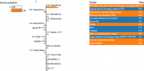
Figure 6. LIME output for an instance classified within the context of renewable energy share prediction
In the given instance (Figure 6), LIME has been applied to elucidate the decision-making process of a model predicting renewable energy share based on several features. The output shows that the model predicts a high likelihood (1.00 probability) that the renewable energy share in total final energy consumption is above a certain threshold, hence classifying this instance into class '1'. The interpretation panel lists the features along with their weights in influencing this particular prediction. Notably, the feature 'Renewable energy share in the total final energy consumption (%)' with a value of 0.34 has the highest positive impact on the prediction, significantly pushing the model towards a classification of '1'. This is visually represented by the bar extending to the right, indicating a strong positive influence. Other features contributing positively, though to a lesser extent, include:
Conversely, features such as 'Electricity from fossil fuels (TWh)' with a value of 0.00 and 'Land Area (Km2)' also at 0.00 exert no discernible negative influence, as indicated by their lack of contribution in the model's decision towards classifying this instance underclass '1'.
The analysis of this LIME output not only validates the model's reliance on logical and expected indicators of renewable energy use but also highlights the complex interplay of various factors that the model considers in its predictions. This transparency aids stakeholders in verifying the model's alignment with intuitive and empirical expectations, enhancing trust and facilitating further refinement of the model based on insights gained from such detailed explanations as shown in Table 4.
Table 4. Summary of ML model performances
|
Model |
Accuracy |
Recall |
Precision |
F1 Score |
Error Rate |
Training Time (s) |
|
LightGBM |
97.40% |
98.29% |
97.10% |
97.69% |
2.60% |
0.126 |
|
XGBoost |
94.66% |
95.60% |
94.90% |
95.25% |
5.34% |
0.158 |
|
AdaBoost |
88.22% |
88.02% |
90.68% |
89.33% |
11.78% |
0.245 |
|
Gradient Boosting |
84.79% |
90.71% |
83.56% |
86.99% |
15.21% |
0.018 |
|
Decision Tree |
84.66% |
76.77% |
94.86% |
84.86% |
15.34% |
0.012 |
|
RF |
82.33% |
75.79% |
91.18% |
82.78% |
17.67% |
0.088 |
|
Extra Trees |
78.49% |
68.46% |
90.91% |
78.10% |
21.51% |
0.155 |
Although the present research aims at the analysis of the performance of single ML models, in further studies it might be worthwhile to investigate model fusion approaches, i.e. ensembles and stacking, in order to integrate the capabilities of various algorithms. These methods can also improve the applicative force and accuracy of the predictions through consolidating the analogous properties and mistake designs of distinct models. Besides, despite the historical nature of the assessment used in the present research, such ML algorithms as LightGBM and XGBoost appear to have high potential to be used in practice in renewable energy short-term and long-term forecasting operations. Their capability to process data that are high dimensional, heterogenous and incomplete makes them appropriate to be used in practical purposes like grid optimization, demand background and energy policy design, where accuracy and reliability are important aspects of concern.
These findings indicate the performance of ML models in forecasting the use of renewable energy and the enhanced performance of predictive analyses and explainability in forecasts due to the implementation of XAI strategies. LightGBM and other models like XGBoost performed well on multivariate energy data, which shows their capabilities to apply in real life energy prediction tasks. The models were guided by the use of the LIME framework, which offered insightful information of factors that were critical predictors, thus generating more trust and enabling wider adoption of AI-based solutions to the energy industry. Such an XAI integration provided a clear and viable method of feature interpretation that can aid analysts and policymakers in propagating data-driven renewable energy policies. The approaches suggested in the current research add to a powerful AI-based forecasting system, boosting the level of transparency and decision-making ability.
A number of technical issues need to be addressed in renewable energy forecasting conditions in real-time: this is a constant flow of streams with live data, consistent updates of the prediction model, and computing limitations. In this dynamic state, securing the stability and reliability of the model involves effective data pipelines, as well as missing or delayed input robustness and periodic retraining with the concept of adapting to the shift in the meaning of the concept. Whereas the current study will use historical information, future research will be undertaken in the formulation of a scalable deployment pattern that can support the formation of the real-time environment with minimal delays and decline in the performance. It would also be useful to add on the existing models by incorporating more data that are detailed and giving explanations that not only have transparency but also action and interpretation. Finally, the optimized models will go far in terms of influencing the real-time renewable energy forecasting, as they will be reliable, explainable and operational to the energy providers and the consumer.
The authors would like to express their sincere appreciation to Jadara University and all colleagues and researchers who provided valuable comments, constructive feedback, and technical insights that contributed to the enhancement of this work's quality. The constructive discussions and critical reviews helped refine the methodology and improve the clarity of the results.
[1] Ridley, M. (2022). Explainable artificial intelligence (XAI): Adoption and advocacy. Information Technology and Libraries, 41(2). https://doi.org/10.6017/ital.v41i2.14683
[2] Ukoba, K., Olatunji, K.O., Adeoye, E., Jen, T.C., Madyira, D.M. (2024). Optimizing renewable energy systems through artificial intelligence: Review and future prospects. Energy & Environment, 35(7): 3833-3879. https://doi.org/10.1177/0958305X241256293
[3] Khalil, R.A.E.H.H., Enjadat, S.M. (2024). Predictive modeling of hourly air temperature based on atmospheric conditions of Karak in Jordan. International Journal of Sustainable Development & Planning, 19(9): 3679-3688. https://doi.org/10.18280/ijsdp.190936
[4] Taşbaşı, D. (2022). Artificial intelligence in the renewable energy industry will exceed $75 billion.
[5] Awad, H., Bayoumi, E.H.E. (2025). Next-generation smart inverters: Bridging AI, cybersecurity, and policy gaps for sustainable energy transition. Technologies, 13(4): 136. https://doi.org/10.3390/technologies13040136
[6] Ghazal, T.M., Abbas, S., Munir, S., Khan, M.A., et al. (2022). Alzheimer disease detection empowered with transfer learning. Computers, Materials & Continua, 70(3): 5005-5019. https://doi.org/10.32604/cmc.2022.020866
[7] Abdel-Jaber, H., Devassy, D., Al Salam, A., Hidaytallah, L., El-Amir, M. (2022). A review of deep learning algorithms and their applications in healthcare. Algorithms, 15(2): 71. https://doi.org/10.3390/a15020071
[8] Ghazal, T.M., Noreen, S., Said, R.A., Khan, M.A., et al. (2022). Energy demand forecasting using fused machine learning approaches. Intelligent Automation & Soft Computing, 31(1): 539-553. https://doi.org/10.32604/iasc.2022.019658
[9] Ghazal, T.M., Munir, S., Abbas, S., Athar, A., et al. (2023). Early detection of autism in children using transfer learning. Intelligent Automation & Soft Computing, 36(1): 11-22. https://doi.org/10.32604/iasc.2023.030125
[10] Tiwari, P., Mehta, S., Sakhuja, N., Kumar, J., Singh, A.K. (2021). Credit card fraud detection using machine learning: A study. arXiv Preprint arXiv: 2108.10005. https://doi.org/10.48550/arXiv.2108.10005
[11] Saleem, M., Abbas, S., Ghazal, T.M., Khan, M.A., et al. (2022). Smart cities: Fusion-based intelligent traffic congestion control system for vehicular networks using machine learning techniques. Egyptian Informatics Journal, 23(3): 417-426. https://doi.org/10.1016/j.eij.2022.03.003
[12] Ghoddusi, H., Creamer, G.G., Rafizadeh, N. (2019). Machine learning in energy economics and finance: A review. Energy Economics, 81: 709-727. https://doi.org/10.1016/j.eneco.2019.05.006
[13] Yang, X.Y., Wang, Z.Y., Zhang, H.X., Ma, N., et al. (2022). A review: Machine learning for combinatorial optimization problems in energy areas. Algorithms, 15(6): 205. https://doi.org/10.3390/a15060205
[14] Kandananond, K. (2019). Electricity demand forecasting in buildings based on ARIMA and ARX models. In Proceedings of the 8th International Conference on Informatics, Environment, Energy and Applications, pp. 268-271. https://doi.org/10.1145/3323716.3323763
[15] Lü, X., Lu, T., Kibert, C.J., Viljanen, M. (2015). Modeling and forecasting energy consumption for heterogeneous buildings using a physical-statistical approach. Applied Energy, 144: 261-275. https://doi.org/10.1016/j.apenergy.2014.12.019
[16] Debnath, K.B., Mourshed, M. (2018). Forecasting methods in energy planning models. Renewable and Sustainable Energy Reviews, 88: 297-325. https://doi.org/10.1016/j.rser.2018.02.002
[17] Goudarzi, S., Anisi, M.H., Kama, N., Doctor, F., et al. (2019). Predictive modelling of building energy consumption based on a hybrid nature-inspired optimization algorithm. Energy and Buildings, 196: 83-93. https://doi.org/10.1016/j.enbuild.2019.05.031
[18] Bertolini, M., Mezzogori, D., Neroni, M., Zammori, F. (2021). Machine learning for industrial applications: A comprehensive literature review. Expert Systems with Applications, 175: 114820. https://doi.org/10.1016/j.eswa.2021.114820
[19] Mosavi, A., Salimi, M., Faizollahzadeh Ardabili, S., Rabczuk, T., et al. (2019). State of the art of machine learning models in energy systems, a systematic review. Energies, 12(7): 1301. https://doi.org/10.3390/en12071301
[20] Luo, B., Wang, H., Liu, H., Li, B., Peng, F. (2018). Early fault detection of machine tools based on deep learning and dynamic identification. IEEE Transactions on Industrial Electronics, 66(1): 509-518. https://doi.org/10.1109/TIE.2018.2807414
[21] Schwendemann, S., Amjad, Z., Sikora, A. (2021). A survey of machine-learning techniques for condition monitoring and predictive maintenance of bearings in grinding machines. Computers in Industry, 125: 103380. https://doi.org/10.1016/j.compind.2020.103380
[22] Loukatos, D., Kondoyanni, M., Alexopoulos, G., Maraveas, C., Arvanitis, K.G. (2023). On-device intelligence for malfunction detection of water pump equipment in agricultural premises: Feasibility and experimentation. Sensors, 23(2): 839. https://doi.org/10.3390/s23020839
[23] He, M., He, D. (2017). Deep learning-based approach for bearing fault diagnosis. IEEE Transactions on Industry Applications, 53(3): 3057-3065. https://doi.org/10.1109/TIA.2017.2661250
[24] Zhou, H., Liu, Q., Yan, K., Du, Y. (2021). Deep learning enhanced solar energy forecasting with AI-driven IoT. Wireless Communications and Mobile Computing, 2021(1): 9249387. https://doi.org/10.1155/2021/9249387
[25] Blasch, E., Li, H.R., Ma, Z.H., Weng, Y. (2021). The powerful use of AI in the energy sector: Intelligent forecasting. arXiv Preprint arXiv: 2111.02026. https://doi.org/10.48550/arXiv.2111.02026
[26] Wang, H., Lei, Z., Zhang, X., Zhou, B., Peng, J. (2019). A review of deep learning for renewable energy forecasting. Energy Conversion and Management, 198: 111799. https://doi.org/10.1016/j.enconman.2019.111799
[27] Wang, F., Zhang, Z.Y., Liu, C., Yu, Y.L., et al. (2019). Generative adversarial networks and convolutional neural networks based weather classification model for day ahead short-term photovoltaic power forecasting. Energy Conversion and Management, 181: 443-462. https://doi.org/10.1016/j.enconman.2018.11.074
[28] Zhang, R.Q., Li, G.Q., Ma, Z.W. (2020). A deep learning based hybrid framework for day-ahead electricity price forecasting. IEEE Access, 8: 143423-143436. https://doi.org/10.1109/ACCESS.2020.3014241
[29] Kim, T.Y., Cho, S.B. (2019). Predicting residential energy consumption using CNN-LSTM neural networks. Energy, 182: 72-81. https://doi.org/10.1016/j.energy.2019.05.230
[30] Kong, W.C., Dong, Z.Y., Jia, Y.W., Hill, D.J., et al. (2017). Short-term residential load forecasting based on LSTM recurrent neural network. IEEE Transactions on Smart Grid, 10(1): 841-851. https://doi.org/10.1109/TSG.2017.2753802
[31] Bourhnane, S., Abid, M.R., Lghoul, R., Zine-Dine, K., et al. (2020). Machine learning for energy consumption prediction and scheduling in smart buildings. SN Applied Sciences, 2(2): 297. https://doi.org/10.1007/s42452-020-2024-9
[32] Wen, L., Zhou, K., Yang, S., Lu, X. (2019). Optimal load dispatch of community microgrid with deep learning based solar power and load forecasting. Energy, 171: 1053-1065. https://doi.org/10.1016/j.energy.2019.01.075
[33] Fan, L.M., Li, J.N., Zhang, X.P. (2020). Load prediction methods using machine learning for home energy management systems based on human behavior patterns recognition. CSEE Journal of Power and Energy Systems, 6(3): 563-571. https://doi.org/10.17775/CSEEJPES.2018.01130
[34] Li, Q., Meng, Q., Cai, J., Yoshino, H., Mochida, A. (2009). Applying support vector machine to predict hourly cooling load in the building. Applied Energy, 86(10): 2249-2256. https://doi.org/10.1016/j.apenergy.2008.11.035
[35] Tanwar, A. (2023). Global data on sustainable energy (2000-2020). Kaggle. https://doi.org/10.34740/KAGGLE/DSV/6327347