Kunal Shejul![]() | R. Harikrishnan*
| R. Harikrishnan*![]() | Rani Fathima
| Rani Fathima![]() | Babul Salam KSM Kader Ibrahim
| Babul Salam KSM Kader Ibrahim![]()
© 2025 The authors. This article is published by IIETA and is licensed under the CC BY 4.0 license (http://creativecommons.org/licenses/by/4.0/).
OPEN ACCESS
The smart-grid-enabled demand-side energy management is used to regulate consumer energy demand. The consumer can adjust their energy consumption in response to the pricing strategy of the grid in the market-based programs. The energy bidding methodology is proposed to predict the electricity rate and optimize the energy demand of the chiller system for energy consumption and cost minimization. The forecasted electricity price and the energy demand schedule generated by the optimization algorithm are used to bid in the electricity market. To forecast the electricity rate, a hybrid model Hilbert Transform-Based Long Short-Term Memory (Hilbert-LSTM) is proposed and the results indicate the improvement in the prediction accuracy in terms of the Mean Absolute Error (MAE), Root Mean Squared Error (RMSE), and Mean Absolute Percentage Error (MAPE). The energy consumption is optimized in the dynamic electricity tariff to generate an optimal energy demand schedule. The bid electricity price is calculated for three different cases and the bidding cost and bidding reliability for the optimized energy demand schedule are compared. The results show that the bidding cost is reduced by 37% and bidding reliability is the highest for the proposed electricity forecasting model Hilbert-LSTM.
Demand Response (DR), electricity bidding, electricity forecasting, energy management, optimization, Genetic Algorithm (GA), JAYA optimization, Real Time Pricing (RTP)
Decisions of the electricity market operators referring to the price at which they sell electricity are increasingly part of the electrical energy management system [1]. Interpreting the data on electricity prices can help electricity operators to make appropriate decisions in due time to enhance their grid performance. Such an approach being driven by electricity price data, requires optimized energy consumption and a balanced allotment of resources. The applications of the Demand Side Management (DSM) in electrical Smart Grid comprise optimizing energy consumption, reduction of peak demand, and integrating renewable energy sources in the grid. The use of advanced metering infrastructure and IoT devices enables the real-time monitoring and control of energy usage [2]. This approach of the system motivates the consumer to make informed decisions about their energy consumption leading to cost minimization. This collectively improves the grid stability and reliability by maintaining a balance between the demand and supply dynamically. In the DSM, there is more focus given on the research on Demand Response (DR) methods and resources to achieve the energy demand peak clipping, valley filling, load shifting, and load conservation for DR development and management with the help of reliability-based programs and market-based programs [3-5]. The immediate near effect of these schemes is the postponement of the need for constructing new power plants alleviating the burden in the short term and easing the gap between the demand and supply side power. The real-time monitoring of the energy consumption and other control parameters with the feedback mechanism can enable timely control adjustments to the demand schedule, ensuring adaptability during contingency circumstances. This inclusion and integration of advanced optimization techniques will certainly revolutionize electrical load management and lead to a sustainable and resilient energy infrastructure.
The significance of this research is that the traditional electricity pricing schemes that offer electricity at fixed tariffs have limited scope to incentivize consumers in the DR programs. The traditional pricing schemes limit the maximum energy demand reduction and load shifting to low energy demand durations, with the proposed methodology discussed in this article this limitation of the traditional pricing scheme is solved. The proposed approach results in significant cost savings and improves the grid reliability by reducing the maximum demand on the grid, which can potentially reduce carbon emissions. The recent developments in the electricity market motivate consumers and power suppliers to purchase and sell electricity at competitive rates. With the electricity rate data available, it is feasible to generate accurate price forecasts that can be used to make informed decisions by consumers and the utilities. The advanced metering infrastructure and the IoT devices are required in the proposed methodology to measure the energy consumption and control the consumer appliances in response to the changes in the electricity prices.
The sustainable approach of the DR programs can be realized potentially with market-based schemes [6, 7]. The increasing challenges in electricity operations need optimal pricing strategies to benefit the consumers and utilities. The authors [8-10] discuss the implementation of the Real Time Pricing (RTP) scheme to reduce the peak demand on the grid. The prediction of electricity prices and load demand is necessary for DR management [11].
The efficient implementation of the DSM programs requires accurate electricity price forecasting. The market operators need a better system forecast to make informed decisions that can maximize the benefits of the stakeholders and enhance the system's reliability. The forecasting techniques are broadly classified as time series models, machine learning and deep learning methods, and hybrid techniques. The authors [12] have used traditional techniques as the Autoregressive (AR) and Autoregressive moving average (ARMA) models, to forecast the spot electricity prices. These methods are used for forecasting univariate time series and for short-term forecasts. The authors used the machine learning techniques of regression to generate the electricity forecasts [13]. The different signal processing technique is used by the authors [14] to decompose and forecast the electricity price with the traditional time series method. The machine learning and deep learning methods with more parameters and better training techniques give better performance than the time series forecasting techniques. The authors [15] compare the different forecasting techniques as the Autoregressive integrated moving average (ARIMA), random forest regression, and neural network models. The authors in their work use techniques as the Long Short-Term Memory (LSTM), and Convolutional Neural Network (CNN)-LSTM to forecast the day-ahead electricity prices [16]. Various researchers have developed hybrid models using the signal processing methods and the traditional time series, machine learning, and deep learning methods [17-20], and improved the deep learning techniques [21, 22].
With the advances in technology with IoT and deregulation of the electricity market, many consumer appliances can be operated with optimal schedules in the smart grid, different control devices and schemes to control the shiftable and non-shiftable loads, where the different consumer appliances that are connected to the grid are controlled based on the energy usage pattern, availability of electricity and consumer preferences [23, 24]. The different appliances with thermal storage capabilities as heaters, air conditioners, HVAC, and battery storage, can be used to minimize the peak electricity load [25, 26]. Different optimization algorithms are used to schedule the loads and optimize the energy consumption [27].
The existing time series forecasting methods discussed are traditional methods that use the techniques to estimate the trend, seasonality, and cyclicity in the time series to forecast. The other techniques as the machine learning based models, intricately model the trends in the time series to estimate the forecast. The proposed method of Empirical Mode Decomposition – Hilbert Transform-Based Long Short-Term Memory (EMD-Hilbert-LSTM) discussed in Section 3.1 has the advantage of decomposing the time series signal in components with different frequency contents and then the LSTM model trains on those inputs, which further improves the prediction accuracy over the traditional LSTM technique and it more intricately models the time series fluctuations.
2.1 Contributions
In this work electricity price forecasting and energy optimization-based electricity bidding methodology is proposed for bidding in the day ahead market. A hybrid electricity rate forecasting model is proposed that combines the EMD method, Hilbert transform, and the LSTM technique. The prediction performance of the forecasting model is compared in terms of the error evaluation metric with the existing algorithms. The prediction performance is improved with the proposed model. Later, the energy demand utilization of the refrigeration system is optimized in the market-based DR program with the Genetic Algorithm-JAYA (GA-JAYA) Algorithm. The refrigeration load energy demand is optimized with the constraints of indoor temperature and power demand. The predicted electricity rate and the generated optimal load schedule are used to bid in the electricity market. The different cases are considered for bidding with the forecasted price. The bidding evaluation comprises 1) the bidding cost calculated for different cases based on the bidding prices quoted for the forecasting algorithms and the optimal chiller plant load schedule generated with the optimization algorithm and 2) the bidding reliability with the different forecasting algorithms. The results indicate that the bid price with the proposed forecasting algorithm EMD-Hilbert-LSTM gives the lowest cost and highest bidding reliability.
The paper is organized as follows: Section 3 discusses the methodology of the research, Section 4 includes the experimental implementation, Section 5 includes the results and discussion, and Section 6 concludes with the summary of the paper.
The proposed methodology integrates the electricity price forecasting model with the energy optimization model to generate an optimal energy consumption schedule. The forecasted electricity price and the energy demand schedule are used to bid in the day-ahead electricity market. The electricity price is highly volatile, non-stationary, and non-linear and requires techniques that can forecast with better accuracy. The literature discusses the different forecasting methods that can be used for forecasting. The authors in this paper develop a hybrid model based on the signal decomposition using the EMD technique and the Hilbert transform to generate the amplitude and frequency spectrum with the LSTM model to forecast the electricity price. The energy demand utilization of the refrigeration system is optimized in the real-time priced program to minimize the cost using the GA-based JAYA optimization algorithm. The generated energy schedule and the predicted electricity price are used to bid in the electricity market. The electricity price data is collected from the electricity power market and is used to generate the electricity price forecast and the optimal energy demand schedule. The forecasted electricity price and the energy demand schedule are used to bid in the electricity market. The consumer and power generators' bids are sorted and selected by the market operator and the Market Clearing Price (MCP) is computed based on the supply and demand equilibrium. The market operator checks for the availability of the transmission corridor and then the selected bids are communicated to the consumers and the power generators. The power generators dispatch the electricity to the distribution station, which is then distributed to the consumers.
3.1 Forecasting of electricity price
3.1.1 EMD
EMD is a technique that is used to analyze complex non-linear and non-stationary signals [28]. The technique involves decomposing the input signal into component signals as the Intrinsic Mode Function (IMF) signals using the decomposition algorithm. The algorithm steps of EMD are as follows,
Step 1. Identify the maxima and minima points of the input signal x(t).
Step 2. Calculate the two function-fitting curves of the upper and lower envelopes with the cubic spline interpolation method.
Step 3. The average value m(t) of the upper and lower envelopes is calculated.
Step 4. The m(t) is subtracted from the input signal to generate a signal c(t).
Step 5. Indicate c(t) as the ith IMF.
The process of calculating the signal m(t) continues until the generated signal c(t) satisfies the IMF conditions given as:
·The number of consecutive extremes and the number of zero crossings must be equal.
·The average of the envelope characterized by the local maxima and minima should be zero.
·The IMFs should have not less than two extreme values either minimum or maximum.
Step 6. The c(t) signal is subtracted from the signal x(t) to generate the residual signal r(t).
Step 7. The residual signal r(t) is used as the input signal and the process to calculate the IMFs is repeated.
Step 8. The process ends when the residual signal has only one maximum or minimum.
The advantage of the EMD technique is that it provides a detailed time-frequency representation of the input signal, representing the fluctuations in the component IMFs and the trend in the residual signal.
3.1.2 Hilbert transform
Hilbert transform is a spectral analysis method to generate the time domain amplitude and frequency spectrum of the input signal [29]. The analytical signal is formed from the input signal and amplitude and frequency are calculated in the time domain.
$H[x(t)]=\int_{-\infty}^{+\infty} \frac{x(t)}{(t-\tau)} d t$ (1)
where, x(t) and H[x(t)] are the complex conjugate pairs, and using the Euler’s identity, z(t) the analytical signal that can be expressed as:
$z(t)=x(t)+j H[x(t)]=a(t) e^{j \phi(t)}$ (2)
where, a(t) is the amplitude and ϕ(t) is the phase angle given by:
$a(t)=\sqrt{x(t)^2+H[x(t)]^2}$ (3)
$\phi(t)=\arctan \frac{H[x(t)]}{x(t)}$ (4)
and ω, the instantaneous frequency is given by:
$\omega=\frac{d \phi(t)}{d t}$ (5)
The Hilbert transform generates the spectrum that is the variation of the instantaneous amplitude and frequency. The Hilbert transform steps are as follows:
Step 1. IMF signals generated with the EMD process are Hilbert transformed with Eq. (1).
Step 2. The analytical signal z(t) is formed with the IMF signal and the complex conjugate Hilbert transformed signal with Eq. (2).
Step 3. The amplitude spectral and frequency spectral is generated with the Eqs. (3)-(5).
The EMD decomposed signal that is Hilbert transformed generates the amplitude and frequency spectrum, this time dependent spectrum data is given as a vector to the LSTM [30] network to train and predict the time series data.
3.2 Energy consumption optimization of the refrigeration system
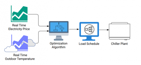
The energy demand utilization of the refrigeration system is optimized for the forecasted electricity price to minimize the chiller plant operating cost. The electricity price that varies for every 15-minute time interval is used to schedule the energy demand of the load for the time intervals that will reduce the operating cost. The DR program in the market-based scheme with the real-time electricity unit rate is used to generate the optimized energy demand schedule. The generated optimal energy demand schedule and the predicted electricity rate are used to bid in the electricity market. Figure 1 depicts the methodology to optimize the energy demand for the chiller plant. The time-varying electricity rate and the outdoor ambient temperature are input to optimize the energy consumption and demand schedule generated for the chiller plant. The optimization problem is solved using the GA-JAYA optimization algorithm.
Figure 1. Input-output flow of the method to optimize the energy consumption
3.2.1 Optimization problem formulation
The optimization problem is formulated for the chiller plant to operate in the real-time priced scheme for reducing the refrigeration system operating cost. The cost function calculates the operating cost based on the time-varying energy consumption and electricity rate during every 15-minute interval.
The mathematical model of the chiller plant is given by the Eq. (6) as follows:
$\begin{gathered}T_{c p}(t+1)= E \times T_{c p}(t)+(1-E)\left[T_o(t)+\left(\operatorname{COP} \times \frac{q_{c p}(t)}{A}\right)\right]\end{gathered}$ (6)
This equation characterizes the indoor temperature of the refrigeration chiller plant based on the power utilization and the outdoor ambient temperature. The indoor temperature Tcp(t+1) for the time slot is a function of the indoor temperature Tcp(t) for the current interval, the outdoor temperature To(t), the power utilized for the time interval qcp(t), the system inertia (E), thermal conductivity (A) and the coefficient of performance (COP).
The indoor temperature variation limit is set by the consumer, that is given by Eqs. (7) and (8) for the minimum and maximum temperatures calculated on the set temperatures of 11℃ and 15℃, respectively. The parameter d is set to 2.
$T_{c p}^{\min }(t)=T_{c p}^{\text {minset }}(t)-d$ (7)
$T_{c p}^{\max }(t)=T_{c p}^{\operatorname{maxset}}(t)+d$ (8)
The objective function is to be solved for the constraints of refrigeration temperature and the rated power limits during every 15-minute time interval. The objective function is the cost calculated for every 15-minute interval, computed with the energy demand and the real-time electricity rate. Eq. (9) is to be solved and the constraints are given by Eqs. (10) and (11).
$\begin{gathered}f=\sum_{t=1}^N \operatorname{Price}(t) \times q_{c p}(t)+B \times \sum_{t=1}^N \mid T_{c p}(t)- T_d(t) \mid\end{gathered}$ (9)
$T_{c p}^{\min }(t)<T_{c p}(t)<T_{c p}^{\max }(t)$ (10)
$0<q_{c p}(t)<q_{c p}^{\max }$ (11)
Eq. (9) combines the operating cost of the refrigeration system and the refrigeration mean set Td temperature deviating component. Td is the mean of the temperatures $T_{c p}^{\min }$ and $T_{c p}^{\max }$. The factor B assigns weight to the temperature divergence component. Larger values of B reduce the temperature divergence more than the cost to be minimized.
The constraints are the refrigeration temperature and the power limits are given by Eqs. (10) and (11) respectively. The optimization problem is solved using the optimization algorithm to calculate the schedule for optimal power consumption. The swarm-based optimization algorithm is used to solve the optimization problem.
3.2.2 GA-JAYA algorithm
The modified optimization algorithm GA-JAYA is a combination of the GA and the JAYA algorithm. The hybrid algorithm uses the GA method to generate the initial solution variables [31]. The GA process of genetic crossover and mutation is used to generate the initial solution by retaining the best sample solutions. The JAYA algorithm [32] is combined with the GA algorithm to solve the optimization problem [33].
$\vec{X}_{\text {new }}=\vec{X}+\vec{r}_1 \cdot\left(\vec{X}_{\text {best }}-\vec{X}\right)-\vec{r}_2 \cdot\left(\vec{X}_{\text {worst }}-\vec{X}\right)$ (12)
The variable vector $\vec{X}$ is used to calculate the new variable $\vec{X}_{\text {new}}$ based on the variables $\vec{X}_{\text {best}}, \vec{X}_{\text {worst}}$ solutions for that iteration that are best and worst, using the random vectors $\overrightarrow{r_1}$ and $\overrightarrow{r_2}$ that are between [0, 1].
The steps for implementing the GA-JAYA algorithm for this energy demand optimization are as follows, where the solution variable is the energy demand of the refrigeration system for the 96-time intervals.
Step 1. The optimization objective function with Eq. (9) is calculated for the GA-generated solutions initially.
Step 2. For every iteration, the best and worst solution is computed and the optimal solution for the iteration is evaluated with Eq. (12).
Step 3. In case the optimal solution in that iteration is better than the solution variable, then it is replaced or else the earlier solution variable is retained.
Step 4. The solution variables are calculated iteratively until the best-performing solution is identified and the iterations are completed.
Step 5. The solution variables are calculated for the objective function that has the constraints of the indoor temperature and the rated power limits.
The advantages of the GA-JAYA algorithm are that the technique combines the solution exploration capabilities of the GA method with the solution exploitation capabilities of the JAYA method. The JAYA method has fewer parameters to control and fewer steps to perform the computation to reach the optimal solution.
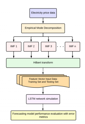
The bidding for electricity in the electricity market requires an accurate prediction of the electricity rate. To predict the electricity rate, the proposed Hilbert-LSTM model is used as the time series electricity price varies non-linearly and is non-stationary [34]. The EMD can decompose the fluctuating and volatile electricity price into detailed IMFs that represent the frequency content in the input signal accurately. The amplitude and frequency time domain spectrum is generated by applying the Hilbert transform to these IMFs. The LSTM network trains on this input data that is Hilbert transformed and can model the time-based dependencies with improved accuracy. Figure 2 depicts the process flow of the electricity rate prediction methodology using the Hilbert-LSTM model.
The LSTM network comprises 50 units, the activation function as ReLu, the optimizer used is the Adam optimizer, and training with the batch size of 32.
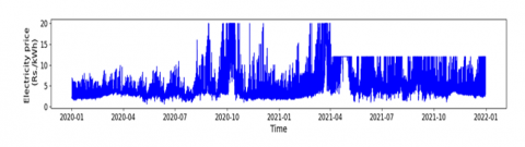
The data collected for the experiment from the electricity market at IEX. There are different mechanisms to trade electricity in the IEX. The different markets that exist are the day ahead market, term ahead market, energy saving, and renewable energy market for the obligations of renewable energy consumption. These markets comprise the total electricity traded at the IEX. This research uses the data collected from the day ahead electricity market. The transactions at the day ahead electricity market take place where the consumers and power suppliers bid for the electricity to be consumed a day in advance. The bidding time horizon is an interval of every 15 minutes for 24 hours in advance to dispatch the electricity for the next day. The buyer and generator bids are made for every 15-minute time slot for 24 hours. Based on the bid price of the sellers and the buyers the market operator then sorts the bids. Based on the cumulative bids, the market supply and demand curves are plotted and the intersection determines the MCP. This process is carried out for every 15-minute time interval and the MCP for the 96-time intervals is determined. Based on the transmission constraints and the availability of power, the MCPs are calculated to dispatch the electricity for the subsequent day. The number of sellers and buyers is large and as the bidding takes place through the closed bidding auction process, the market clearing rate varies non-linearly and the electricity rate prediction is necessary for accurate electricity market bidding for the improvement of the bidding reliability and the buyers' cost benefit. Figure 3 depicts the actual electricity rate obtained from IEX. The electricity rate data is preliminarily standardized with the Min-Max scaling method and a vector is formed to be given as input to the forecasting model.
Figure 2. Block diagram for the methodology to predict the electricity rate
Figure 3. The actual electricity rate data collected from IEX
The model of Hilbert-LSTM is proposed to forecast the electricity rate in the electricity market. The electricity price data is collected and given as input to the model to predict the electricity rate.
The next process is to improve the energy demand of the refrigeration system in the real-time priced program to reduce the operating cost. The chiller plant has to consume electricity to maintain the refrigeration temperature in the temperature constraints. The GA-JAYA optimization algorithm is used to generate the energy demand to minimize the cost.
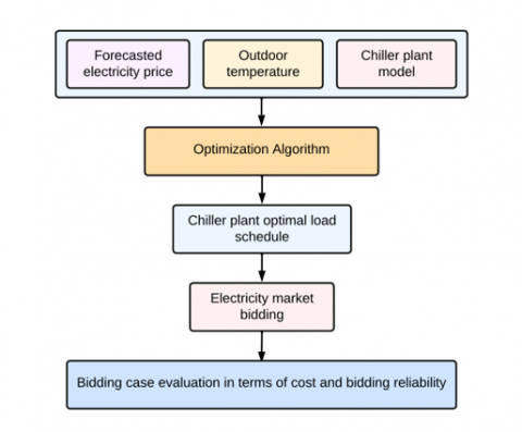
Figure 4 depicts the process flow of bidding in the electricity market using the forecasted electricity price and the optimized chiller plant demand schedule. The optimization process calculates the optimized energy consumption for operating the refrigeration system. This demand schedule and the predicted electricity rate are used for bidding. The bidding cost for the forecasting algorithm and the bidding reliability are evaluated.
The simulations are performed in Google Colab and with the MATLAB 2023 software. The temperature data is collected from the weather data website [35] and the electricity rate data is obtained from the IEX day ahead electricity market [36]. All the data used in this research are publicly available and referred from the public database [37].
Figure 4. Block diagram for energy demand optimizer and bid for electricity in the electricity market
5.1 Data collection
The methodology is validated with the electricity rate data obtained from the IEX electricity market. Initially, the electricity price prediction is performed with the proposed forecasting model of Hilbert-LSTM and the prediction performance is evaluated with the error evaluation metrics. The dataset is collected for the duration of two years from January 2020 to December 2022. The electricity price is available for every 15-minute time interval for 24 hours in a day, and the total dataset comprises of 70,000 data points of univariate time-varying electricity prices. The dataset used to train the forecasting algorithm is divided into an 80% training dataset and a 20% testing dataset.
5.2 Evaluation metrics
The forecasting performance is evaluated using the error metrics of Mean Absolute Error (MAE), Root Mean Squared Error (RMSE), and Mean Absolute Percentage Error (MAPE) and calculated as given by the following equations:
$\begin{aligned} \mathrm{MAE} & =\frac{1}{n} \sum_{i=1}^n\left|x_i-\hat{x}_i\right| \\ \mathrm{RMSE} & =\sqrt{\frac{1}{n} \sum_{i=1}^n\left(x_i-\hat{x}_i\right)^2} \\ \mathrm{MAPE} & =\frac{1}{n} \sum_{i=1}^n\left|\frac{x_i-\hat{x}_i}{x_i}\right| \times 100\end{aligned}$
where, the xi is the actual data value, $\widehat{x}_i$ is the predicted data value, n is the total number of data points.
5.3 Forecasting of electricity price from the Indian electricity market
The electricity price data collected from the day ahead electricity market from IEX is real-time varying. The time series data varies non-linearly and is non-stationary. The large number of sellers and consumers that bid for varying amounts of electricity power to be sold or purchased at a variable price makes the MCP highly volatile. The bidding process, which is a double-sided closed auction makes it difficult for the consumers and the sellers to understand the appropriate bid price to be quoted. The proposed methodology in this paper initially predicts the electricity rate using the modified method of Hilbert-LSTM.
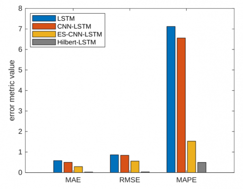
The prediction accuracy is measured with the metrics and compared with different forecasting algorithms, as shown in Table 1. The proposed forecasting model Hilbert-LSTM forecasts with higher accuracy as compared to the existing algorithms of LSTM, CNN-LSTM and ES-CNN-LSTM [38], with the error metrics of MAE as 0.02691, RMSE as 0.03265, and MAPE as 0.4954%. The prediction results with the metrics are depicted in Figure 5. The prediction models LSTM and CNN-LSTM are selected as the proposed model Hilbert-LSTM is developed using the LSTM model and the CNN-LSTM is another model developed with LSTM that is used popularly for time series forecasting.
Table 1. The prediction results for the different models in terms of various metrics
|
Model |
R Squared |
MAE |
RMSE |
MAPE |
|
LSTM |
0.9496 |
0.5849 |
0.8644 |
7.12 |
|
CNN-LSTM |
0.9472 |
0.4989 |
0.8425 |
6.56 |
|
ES-CNN-LSTM |
0.9964 |
0.2905 |
0.5602 |
1.53 |
|
Hilbert-LSTM |
0.9998 |
0.02691 |
0.03265 |
0.4954 |
Figure 5. The evaluation metrics-based prediction results for forecasting models
The prediction accuracy of the forecasting algorithms is validated using the Diebold-Mariano (DM) test [39]. Table 2 shows the DM test findings as the p-values computed from the prediction error. The null hypothesis is that the forecasting accuracy between the method in the row and the method in the column has no significant difference. The p-values less than 0.05 significant value indicate that the forecasting accuracy of the method in the column is less than the method in the row. The DM test results indicate that the Hilbert-LSTM model performs better than the LSTM and CNN-LSTM and ES-CNN-LSTM models.
Table 2. DM test findings as the p-values
|
Model |
LSTM |
CNN-LSTM |
ES-CNN-LSTM |
Hilbert-LSTM |
|
LSTM |
– |
0.77712 |
0.99794 |
0.99791 |
|
CNN-LSTM |
0.22288 |
– |
0.99794 |
0.99789 |
|
ES-CNN-LSTM |
< 0.00206 |
< 0.00206 |
– |
0.99621 |
|
Hilbert-LSTM |
< 0.00209 |
< 0.00211 |
< 0.0039 |
– |
5.4 Optimization of energy demand for the refrigeration system
The proposed methodology to optimize the energy consumption based on the day ahead forecasted electricity price is used for the refrigeration chiller plants. The forecasted electricity price is used to optimize the energy demand for 24 hours in a day. The optimization problem to generate the energy consumption of chiller plants with the constraints of temperature limits and the power consumption rating limits is solved using the GA-JAYA optimization algorithm. The inputs to the optimization algorithm are the outdoor ambient temperature and the forecasted electricity price. Table 3 shows the chiller plant attributes that are used in the simulation. The power demand with the normal method operates the chiller plant to maintain the refrigeration temperature in the consumer-set temperature limits without energy consumption optimization. The power demand with the algorithm is within the limits of the rating of the refrigeration system and is optimized to shift the demand from the high-rate durations to the low-rate durations.
Table 3. Refrigeration system parameters
|
Attribute |
Value |
|
Power rating (Q) |
3.5 (kW) |
|
System inertia (E) |
0.93 (p.u.) |
|
Thermal conductivity (A) |
0.18 (kW/℃) |
|
Coefficient of performance (COP) |
2.5 (p.u.) |
Table 3 shows the chiller plant attributes [33]. The algorithm simulation parameters are set as follows, for the GA algorithm the crossover process is performed for 80% initial population and the mutation process for the remaining 20% initial population. The number of particles for the JAYA and GA-JAYA algorithms is 150 and the number of iterations is 12. The parameters of the algorithm r1, r2 vary in the limits of [0, 1].
Table 4 shows the results of the GA-JAYA algorithm that are compared with the JAYA algorithm, Grey Wolf Optimizer (GWO), and the ON/ OFF method. The results indicate that the operating cost of the refrigeration system is lowest for the GA-JAYA algorithm with Rs. 105.77. The energy consumption is 65.48 kWh and is reduced compared to the normal operation and the GWO algorithm and slightly greater than the JAYA algorithm. The reduced consumption indicates considerable energy savings. The results show that with the GA-JAYA algorithm, the energy consumption is increased the highest during the low-price hours. This improvement in the shift of energy consumption indicates that the DR objective to shift the energy utilization from the high-price hours that represent the high demand durations to the low-price hours is achieved. The power demand schedule generated with the optimization algorithm is used as the demand schedule for bidding in the day-ahead electricity market at IEX.
Table 4. The results of simulation for different algorithms for different parameters
|
Algorithm |
Cost (Rs.) |
Energy Consumption (kWh) |
Energy Consumption Variation (%) |
Ti Mean Deviation (%) |
|
|
Peak Hours |
Off Peak Hours |
||||
|
Normal |
136.26 |
73.50 |
49.70 |
54.67 |
-0.51 |
|
GWO |
113.59 |
69.19 |
40.72 |
59.28 |
2.86 |
|
JAYA |
109.3 |
63.68 |
46.08 |
53.92 |
5.12 |
|
GA-JAYA |
105.77 |
65.48 |
39.23 |
60.77 |
4.25 |
Table 5. Simulation results for the cost and number of selected bids for forecasting models
|
Model |
Cost (Rs.) |
Number of Bids Selected |
|||||
|
Normal |
Case 1 |
Case 2 |
Case 3 |
Case 1 |
Case 2 |
Case 3 |
|
|
LSTM |
149.00 |
133.85 |
116.77 |
116.93 |
34 |
88 |
62 |
|
CNN-LSTM |
141.77 |
122.90 |
117.46 |
111.92 |
46 |
89 |
62 |
|
ES-CNN-LSTM |
118.51 |
111.41 |
122.61 |
108.73 |
55 |
84 |
67 |
|
Hilbert-LSTM |
114.56 |
96.79 |
104.65 |
100.15 |
74 |
95 |
81 |
5.5 Bidding in the IEX electricity market based on the forecasted electricity price
The bidding process in the IEX market comprises of the market participating bidder submitting their bids of the power demand requirement and power demand-supply with the bid quote price for every 15 minutes at 96-time intervals for the day. The case study in this paper discusses the energy optimization of the chilling system based on the forecasted electricity price. The power consumption schedule generated by the proposed algorithm calculates the energy consumption during every 15-minute interval for the day. The price forecasted by the proposed forecasting algorithm and the energy consumption demand are used for bidding in the IEX. The bids made by the different consumers and sellers are sorted by the market operator. The consumer and the seller bids are selected depending on the supply and demand equilibrium, where the intersection of the supply and demand curves determines the MCP. This MCP is calculated for every 15-minute interval for the day. The bids made by the buyer with the quoted bid price that is above the MCP get selected. The bid is not selected if the quoted bid price is not greater than the MCP and the consumers are charged based on the tariff of the distribution company for any consumption during that interval where the bid is not selected. The different cases are discussed as follows the bidding at the forecasted electricity price, the bidding at the base maximum price increment, and the bidding at the base minimum price increment. The demand schedule generated by the optimization algorithm is used as the energy demand bid in every case for all the forecasting algorithms.
5.5.1 Case 1: Bidding at the forecasted price
The bids for the electricity demand in the IEX are made based on the electricity price forecasted by the prediction model Hilbert-LSTM and the cost incurred is compared with the models LSTM, CNN-LSTM and ES-CNN-LSTM. The results for the cost of the different forecasting algorithms generated bid price with the optimized energy bid calculated by the GA-JAYA optimization algorithm are shown in Table 5. The results indicate that the cost for the bids made with the proposed model Hilbert-LSTM is the lowest. The results also show the number of times the bids are selected for the algorithms that indicates that the bids selected for the proposed model Hilbert-LSTM are the largest.
5.5.2 Case 2: Bidding at the base maximum price increment
The bids in this case are made with the incremented forecasted electricity prices. The forecasted prices are incremented throughout with the factor of the percentage of the MAPE of the maximum of the forecasted electricity price values. The results for the cost for the bids made in this case are shown in Table 5 for the forecasting models and the results indicate that the cost is lowest for the Hilbert-LSTM model. The results also show the number of times the bids are selected for the algorithms that indicates that the bids selected for the proposed model Hilbert-LSTM are the largest.
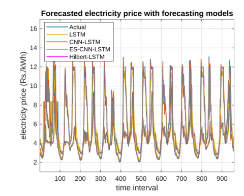
(a) The actual electricity rate and forecasted electricity rate with the forecasting models for day ahead prediction
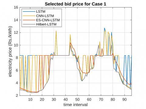
(b) The selected bid price for the forecasting models for Case 1 with the actual forecasted price
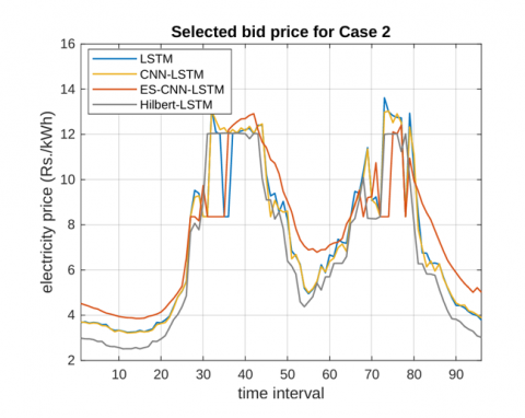
(c) The selected bid price for the forecasting models for Case 2 with a base maximum price increment
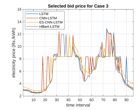
(d) The selected bid price for the forecasting models for Case 3 with a base minimum price increment
Figure 6. The simulation results
5.5.3 Case 3: Bidding at the base minimum price increment
The forecasted prices are incremented throughout with the factor of the MAPE of the minimum of the forecasted electricity price values by the prediction algorithms. This price is used as the bid price and the cost for the different forecasting models are shown in Table 5. The results indicate that the cost for the Hilbert-LSTM model is the lowest. The results also show that the number of times the bids are selected for the proposed model Hilbert-LSTM is the largest.
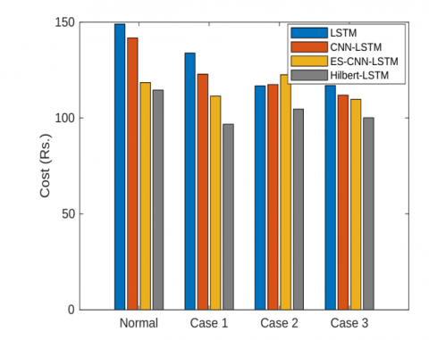
Figure 7. The bidding cost for operating the chiller plant for forecasting algorithms for the different cases
The results for the cost with the bids made by the buyers in the IEX electricity market dependent on the forecasted electricity rate and with the case of bids made with base maximum price increment and base minimum price increment are also compared with the cost for normal operation of the refrigeration system load with the fixed tariff of the electricity distribution company and with the actual real-time priced electricity. The cost for the normal operation of the refrigeration load with the fixed tariff of the electricity distribution company, where the energy is not optimized with the optimization algorithm is Rs. 153.62. Whereas the cost for normal operation of the load with forecasted electricity price with prediction models is Rs. 114.56 for Hilbert-LSTM, Rs. 118.51 for ES-CNN-LSTM, Rs. 141.77 for CNN-LSTM, and Rs. 149 for LSTM. The cost for the bids made with the forecasted electricity price and energy-optimized demand bids is Rs. 96.79 for the proposed Hilbert-LSTM model, Rs. 111.41 for ES-CNN-LSTM, Rs. 122.90 for the CNN-LSTM model and Rs. 133.85 for the LSTM model. The cost for the bids made with the quoted bid price of base maximum price increment is Rs. 104.65 for Hilbert-LSTM, Rs. 122.61 for ES-CNN-LSTM, Rs. 117.46 for CNN-LSTM, and Rs. 116.77 for LSTM. The cost for the bids made with the quoted bid price of base minimum price increment is Rs. 100.15 for Hilbert-LSTM, Rs. 108.73 for ES-CNN-LSTM, Rs. 111.92 for CNN-LSTM, and Rs. 116.93 for LSTM. The results for the proposed methodology of electricity forecasting and energy optimization are comparatively better in terms of operating cost. Compared to the fixed electricity tariff the bidding with the proposed Hilbert-LSTM and optimized energy schedule reduced the cost by 37%.
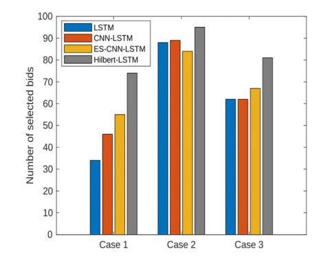
Figure 8. The number of bids selected in the bidding with the bid price quoted with the electricity price forecasting algorithms for different cases
The energy optimization shifts the energy consumption from the high rate durations to the low rate durations, which reduces the cost. The bidding process is opaque, where the buyers have to bid with the price that will be selected only if the quoted bid price is higher than the MCP computed after the entire bidding process is complete. Therefore, bidding with the price forecasted with the accurate prediction model can increase the chances of the bids getting selected. The bid price made with the forecasted models and the bid selected price is shown in Figure 6 for Case 1, Case 2, and Case 3 that also shows the forecasted electricity prices with different forecasting models. The consumers have to purchase the power at the fixed tariff of the electricity distribution company if the bid for a particular time interval is not selected and the fixed tariff is Rs. 8.36. Figure 7 depicts the bidding costs for operating the chiller plant for the forecasting models with different cases. The cost for the bids made with the proposed forecasting model of Hilbert-LSTM is the lowest for Case 1 and lower for Case 3 than Case 2 and the normal method. The costs for the bids made with the proposed Hilbert-LSTM models are lower than the ES-CNN-LSTM, CNN-LSTM and LSTM models for all the cases.
The bids are made for every 15-minute time interval for the day for 96-time intervals. The bidding reliability is compared for the forecasting algorithm for different cases in Figure 8 and it can be seen that the number of bids that are selected are the highest for the Hilbert-LSTM model than the ES-CNN-LSTM, CNN-LSTM and LSTM models for Case 1, Case 2, and Case 3.
The proposed methodology that predicts the electricity price and optimizes the energy demand schedule reduces the cost and also improves the bidding reliability that establishes the correlation and causality between the optimized energy demand schedule and the cost savings. The energy optimization with higher efficiency directly increases the cost savings.
The deregulated short-term electricity market where the sellers and buyers can bid for the electricity has increased number of bids from the participants that has made the bid selection process complex due to the closed bidding process and the MCP being volatile, non-stationary, and non-linear. This requires the bidder to have an accurate forecast of the day ahead electricity price to accurately bid in the electricity market. This paper proposes a methodology that forecasts electricity prices and optimizes the energy demand for electricity market bidding. A hybrid model Hilbert-LSTM is proposed to forecast the electricity price that combines the methods of signal decomposition using the EMD and forecasting with the LSTM model. The EMD decomposed component signals are given to the LSTM network to train and forecast, which uses the advantages of the LSTM model to intricately model the temporal dependencies in the time series. The Hilbert-LSTM model forecasts the electricity price with better accuracy with the MAE as 0.02691, RMSE as 0.03265, and MAPE as 0.4954. The forecasted electricity price is used to optimize the energy demand with the GA-JAYA algorithm and to minimize the operating cost of the refrigeration system.
The forecasted electricity price and the optimized energy demand are used to bid for electricity in the day-ahead electricity market at IEX. The performance of the bidding with the proposed forecasting models is evaluated in terms of the cost. The costs for different bidding cases are compared with the forecasting models and the results indicate that the bids made with the price forecasted with the Hilbert-LSTM model are selected the highest number of times and have the lowest cost. The bidding cost is reduced by 37% as compared to the fixed electricity tariff.
The advantages of minimizing the overall electricity demand on the electrical grid and improving the grid reliability can be achieved with energy optimization by increasing consumer participation to optimally schedule their electricity demand.
The future scope of this research includes developing accurate forecasting and optimization methods.
|
Abbreviations |
|
|
DR |
Demand Response |
|
CNN |
Convolutional Neural Network |
|
EMD |
Empirical Mode Decomposition |
|
ES |
Exponential Smoothing |
|
IMF |
Intrinsic Mode Function |
|
LSTM |
Long Short-Term Memory |
|
GA |
Genetic Algorithm |
|
GA-JAYA |
Genetic Algorithm-JAYA Algorithm |
|
RTP |
Real Time Pricing |
|
Symbols and parameters |
|
|
A |
thermal conductivity |
|
COP |
coefficient of performance |
|
E |
system inertia |
|
qcp |
electricity power utilization of chiller plant |
|
$q_{c p}^{\max }$ |
maximum rated power of the chiller plant |
|
t |
time slot |
|
Tcp |
temperature maintained by chiller plant |
|
$T_{c p}^{\text {min}}$ |
minimum temperature of chiller plant |
|
$T_{c p}^{\text {max}}$ |
maximum temperature of chiller plant |
|
$T_{c p}^{\text {minset}}$ |
chiller plant minimum set temperature |
|
$T_{c p}^{\text {maxset}}$ |
chiller plant maximum set temperature |
|
To |
outdoor ambient temperature |
[1] Panda, S., Mohanty, S., Rout, P.K., Sahu, B.K., et al. (2023). A comprehensive review on demand side management and market design for renewable energy support and integration. Energy Reports, 10: 2228-2250. https://doi.org/10.1016/j.egyr.2023.09.049
[2] Depuru, S.S.S.R., Wang, L., Devabhaktuni, V., Gudi, N. (2011). Smart meters for power grid—Challenges, issues, advantages and status. Sustainable Energy Reviews, 15(6): 2736-2742. https://doi.org/10.1016/j.rser.2011.02.039
[3] Jeyaranjani, J., Devaraj, D. (2022). Improved genetic algorithm for optimal demand response in smart grid. Sustainable Computing: Informatics and Systems, 35: 100710. https://doi.org/10.1016/j.suscom.2022.100710
[4] Wang, C., Chen, S., Mei, S., Chen, R., et al. (2020). Optimal scheduling for integrated energy system considering scheduling elasticity of electric and thermal loads. IEEE Access, 8: 202933-202945. https://doi.org/10.1109/ACCESS.2020.3035585
[5] Lin, S., Lin, M., Shen, Y., Li, D. (2022). An optimal scheduling strategy for integrated energy systems using demand response. Frontiers in Energy Research, 10: 920441. https://doi.org/10.3389/fenrg.2022.920441
[6] Elma, O., Taşcıkaraoğlu, A., İnce, A.T., Selamoğulları, U.S. (2017). Implementation of a dynamic energy management system using real time pricing and local renewable energy generation forecasts. Energy, 134: 206-220. https://doi.org/10.1016/j.energy.2017.06.011
[7] Gianfreda, A., Parisio, L., Pelagatti, M. (2016). The impact of RES in the Italian day-ahead and balancing markets. The Energy Journal, 37(2_suppl): 161-184. https://doi.org/10.5547/01956574.37.SI2.agia
[8] Nebey, A.H. (2024). Recent advancement in demand side energy management system for optimal energy utilization. Energy Reports, 11: 5422-5435. https://doi.org/10.1016/j.egyr.2024.05.028
[9] Yang, H., Chen, Q., Liu, Y., Ma, Y., et al. (2024). Demand response strategy of user-side energy storage system and its application to reliability improvement. Journal of Energy Storage, 92: 112150. https://doi.org/10.1016/j.est.2024.112150
[10] Yang, H., Zhang, Y., Ma, Y., Zhou, M., et al. (2019). Reliability evaluation of power systems in the presence of energy storage system as demand management resource. International Journal of Electrical Power & Energy Systems, 110: 1-10. https://doi.org/10.1016/j.ijepes.2019.02.042
[11] Chan, S.C., Tsui, K.M., Wu, H.C., Hou, Y., et al. (2012). Load/price forecasting and managing demand response for smart grids: Methodologies and challenges. IEEE signal processing magazine, 29(5): 68-85. https://doi.org/10.1109/MSP.2012.2186531
[12] Cuaresma, J.C., Hlouskova, J., Kossmeier, S., Obersteiner, M. (2004). Forecasting electricity spot-prices using linear univariate time-series models. Applied Energy, 77(1): 87-106. https://doi.org/10.1016/S0306-2619(03)00096-5
[13] Nogales, F.J., Contreras, J., Conejo, A.J., Espínola, R. (2002). Forecasting next-day electricity prices by time series models. IEEE Transactions on Power Systems, 17(2): 342-348. https://doi.org/10.1109/TPWRS.2002.1007902
[14] Conejo, A.J., Plazas, M.A., Espinola, R., Molina, A.B. (2005). Day-ahead electricity price forecasting using the wavelet transform and ARIMA models. IEEE transactions on Power Systems, 20(2): 1035-1042. https://doi.org/10.1109/TPWRS.2005.846054
[15] Rawal, K., Ahmad, A. (2022). Day-ahead market electricity price prediction using time series forecasting. In 2022 1st International Conference on Sustainable Technology for Power and Energy Systems (STPES), Srinagar, India, pp. 1-6. https://doi.org/10.1109/STPES54845.2022.10006455
[16] Bozlak, Ç.B., Yaşar, C.F. (2024). An optimized deep learning approach for forecasting day-ahead electricity prices. Electric Power Systems Research, 229: 110129. https://doi.org/10.1016/j.epsr.2024.110129
[17] Xiong, X., Qing, G. (2023). A hybrid day-ahead electricity price forecasting framework based on time series. Energy, 264: 126099. https://doi.org/10.1016/j.energy.2022.126099
[18] Zhang, J., Tan, Z., Wei, Y. (2020). An adaptive hybrid model for short term electricity price forecasting. Applied Energy, 258: 114087. https://doi.org/10.1016/j.apenergy.2019.114087
[19] Zhang, J.L., Zhang, Y.J., Li, D.Z., Tan, Z.F., et al. (2019). Forecasting day-ahead electricity prices using a new integrated model. International Journal of Electrical Power & Energy Systems, 105: 541-548. https://doi.org/10.1016/j.ijepes.2018.08.025
[20] Wu, C., Wang, J., Chen, X., Du, P., et al. (2020). A novel hybrid system based on multi-objective optimization for wind speed forecasting. Renewable Energy, 146: 149-165. https://doi.org/10.1016/j.renene.2019.04.157
[21] Yang, H., Schell, K.R. (2022). GHTnet: Tri-Branch deep learning network for real-time electricity price forecasting. Energy, 238: 122052. https://doi.org/10.1016/j.energy.2021.122052
[22] Lehna, M., Scheller, F., Herwartz, H. (2022). Forecasting day-ahead electricity prices: A comparison of time series and neural network models taking external regressors into account. Energy Economics, 106: 105742. https://doi.org/10.1016/j.eneco.2021.105742
[23] Essiet, I.O., Sun, Y., Wang, Z. (2019). Optimized energy consumption model for smart home using improved differential evolution algorithm. Energy, 172: 354-365. https://doi.org/10.1016/j.energy.2019.01.137
[24] Ahmad, M.W., Mourshed, M., Mundow, D., Sisinni, M., et al. (2016). Building energy metering and environmental monitoring – A state-of-the-art review and directions for future research. Energy and Buildings, 120: 85-102. https://doi.org/10.1016/j.enbuild.2016.03.059
[25] Chakraborty, N., Mondal, A., Mondal, S. (2020). Efficient load control based demand side management schemes towards a smart energy grid system. Sustainable Cities and Society, 59: 102175. https://doi.org/10.1016/j.scs.2020.102175
[26] Rocha, H.R., Honorato, I.H., Fiorotti, R., Celeste, W.C., et al. (2021). An Artificial Intelligence based scheduling algorithm for demand-side energy management in Smart Homes. Applied Energy, 282(Part A): 116145. https://doi.org/10.1016/j.apenergy.2020.116145
[27] Alshammari, N., Asumadu, J. (2020). Optimum unit sizing of hybrid renewable energy system utilizing harmony search, Jaya and particle swarm optimization algorithms. Sustainable Cities and Society, 60: 102255. https://doi.org/10.1016/j.scs.2020.102255
[28] Wang, G., Chen, X.Y., Qiao, F.L., Wu, Z., et al. (2010). On intrinsic mode function. Advances in Adaptive Data Analysis, 2(3): 277-293. https://doi.org/10.1142/S1793536910000549
[29] de Souza, U.B., Escola, J.P.L., da Cunha Brito, L. (2022). A survey on Hilbert-Huang transform: Evolution, challenges and solutions. Digital Signal Processing, 120: 103292. https://doi.org/10.1016/j.dsp.2021.103292
[30] Hochreiter, S., Schmidhuber, J. (1997). Long short-term memory. Neural Computation, 9(8): 1735-1780. https://doi.org/10.1162/neco.1997.9.8.1735
[31] McCall, J. (2005). Genetic algorithms for modelling and optimisation. Journal of computational and Applied Mathematics, 184(1): 205-222. https://doi.org/10.1016/j.cam.2004.07.034
[32] Rao, R. (2016). Jaya: A simple and new optimization algorithm for solving constrained and unconstrained optimization problems. International Journal of Industrial Engineering Computations, 7(1): 19-34. http://doi.org/10.5267/j.ijiec.2015.8.004
[33] Shejul, K., Harikrishnan, R. (2024). Energy consumption optimization of chiller plants with the genetic algorithm based GWO and JAYA algorithm in the dynamic pricing demand response. Results in Engineering, 22: 102193. https://doi.org/10.1016/j.rineng.2024.102193
[34] Shejul, K., Harikrishnan, R., Kukker, A. (2024). Short-term electricity price forecasting using the empirical mode decomposed Hilbert-LSTM and Wavelet-LSTM models. Journal of Electrical and Computer Engineering, 2024(1): 4575735. https://doi.org/10.1155/jece/4575735
[35] AccuWeather. https://www.accuweather.com/.
[36] Indian Energy Exchange (IEX). https://www.iexindia.com/.
[37] Shejul, K. (2024). Day ahead electricity price data. Mendeley Data, V1. https://doi.org/10.17632/7t5jg4ms99.1
[38] Shejul, K., Harikrishnan, R., Gupta, H. (2024). The improved integrated Exponential Smoothing based CNN-LSTM algorithm to forecast the day ahead electricity price. MethodsX, 13: 102923. https://doi.org/10.1016/j.mex.2024.102923
[39] Diebold, F.X., Mariano, R.S. (1995). Comparing predictive accuracy. Journal of Business & Economic Statistics, 13(3): 253-263. http://stat.wharton.upenn.edu/~steele/Courses/434/434Context/BackTesting/DieboldMariano95.pdf.