Seyed Matin Malakouti
© 2023 IIETA. This article is published by IIETA and is licensed under the CC BY 4.0 license (http://creativecommons.org/licenses/by/4.0/).
OPEN ACCESS
Due to the speeding up of climate change, there is an urgent need to switch from using fossil fuels to producing energy using renewable energy sources. This change has to happen as soon as feasibly possible. Thus, in this article, to forecast wind speed and wind energy output in Turkey, the Light Gradient Boosting Machine (LightGBM) approach was applied, the hyperparameters of the LightGBM were tuned to the grid search method, and finally some evaluation criteria such as root mean square error and R2 were calculated to show the performances of the LightGBM. Fortunately, an R2 value of 0.98 for forecasting wind speed was found after 25 s. Additionally, the assessment criterion R2 =1 for predicting the production power of the wind turbine was attained after 90 s.
grid search method, light gradient boosting machine, SCADA system, wind turbine
In the contemporary electricity grid, wind turbine systems are now often seen, and their use is only growing on a worldwide scale. The United States Department of Energy set the 2030 goal of generating 20% of its power from wind resources [1] in 2008. According to an Inter- national Energy Agency estimate, 10,800 GW of renewable energy will be available globally by the year 2040 [2]. Most wind farms are in distant areas or offshore owing to their enormous size since they are bound by the right-of-way privileges of regional and local governments [3]. To install towers optimally for optimum wind power collection, wind farms also need to thoroughly analyze the wind currents across potential sites, according to [4]. Effective control of each wind turbine is crucial for increasing both efficiency and profitability for power suppliers because of the complexity and size of the electrical architecture of wind farms [5]. To maximize the quantity of electricity generated from wind turbines and to minimize the time a wind turbine is offline due to damage, the remote control and monitoring systems for grid-connected wind farms are indispensable. Artificial intelligence (AI) and machine learning (ML) methods have been used by experts to assist with the forecast of wind turbine systems [6-10].
Effective wind power forecasting is essential for operators to incorporate wind turbines in smart grids and enhance power output control. The literature contains some data-driven methods to improve wind power prediction. Short-term wind power forecasting has tradition- ally been done using time-series techniques, such as the autoregressive moving average (ARMA) model and its variations [11, 12]. The approach in [11] forecasted hourly wind power using an ARMA model. It showed predicting solid ability 1 hour ahead, decreasing precision as time passed. A combined technique merging an ARMA and an Artificial neural network has been suggested in [12] to expect wind energy over the near term. This research shows that the coupled strategy outperformed the solo ARMA and Artificial neural network in predicting performance.
Many ML approaches for predicting wind power have been developed in recent decades. A Gaussian process-based wind power forecasting technique based on numerical weather forecasting has been suggested [13]. Azimi et al. [14] examined the K-means clustering approach with a cluster selection algorithm for enhancing feature extraction from wind time-series data. Yang et al. [15] presented an support vector machine-enhanced Markov technique for predicting short-term wind power. Because of its flexibility and capacity to describe process nonlinearity, the research of Ti et al. [16] showed that an ANN model accurately forecasted wind power and outperformed analytical models. In the study of Malakouti et al. [17], the performance of different algorithms such as CNN-LSTM, ensemble, and predicting the production power of the Texas wind farm was examined. Also, in the study of Malakouti [18], the author investigated the performance of several ML methods in terms of algorithm execution time and their accuracy in predicting the production power of a supervisory control and data acquisition (SCADA) system.
2.1 Data preparation
The data used in this paper are taken from the SCADA system in Turkey [19]. The data comprise attributes as below:
LV Active Power (kW), Wind Speed (m/s), Wind Direction (°), and Theoretical Power (kW).
2.2 Light gradient boosting machine
The light gradient boosting machine (LightGBM) system uses decision tree methods as its foundation. While previous ensemble learning algorithms utilize the level-wise (or depth- wise) approach to form the trees, this technique uses the leaf-wise (or best-first) strategy. Gradient-Based One-Side Sampling (GOSS) and Exclusive Feature Bundling (EFB) are two cutting-edge methods that LightGBM uses. Because GOSS employs a subset of more minor instances rather than all instances, and EFB may combine exclusive features into less dense ones, the computing cost is decreased using these unique approaches.
LightGBM tries to find a particular function $\hat{g}(x)$ that minimizes the loss function $L(y, g(x))$ given the training set $X=\left(x_i,, Y i\right)_{i=1}^n$ as below:
$\hat{g}=\arg \min E_{x, y}[L(y, g(x))]$ (1)
LightGBM uses a combination of T regressor trees for finding the final algorithm as below:
$g_T(x)=\sum_{t=1}^T g_t(x)$ (2)
The function $w_p(x), p \in(1,2, \ldots, M)$ defines regression trees, where M is the amount of tree leaves, p is the decision rule of trees, and w is the leaf node sample weight.
At step t, the algorithm trains according to:
$\Gamma_t=\sum_{j=1}^J\left(\sum_{i \in I_j} f_i\right) w_j+\frac{1}{2}\left(\sum_{i \in I_j} h_i+\lambda\right) w_j^2$ (3)
where, fi and hi are, respectively, the 1st-order and 2nd-order gradients of the loss function, Ij is the leaf j sample set, and γ an increase in the constant value that prevents the 2nd term from becoming 0.
The optimal leaf weight scores of each leaf node $w_i^*$ and the extreme value of ΓKare obtained for a particular tree structure p(x) using the relations:
$w_j^*=-\frac{\sum_{i \in I_j} f_i}{\sum_{i \in I_j} h_i+\lambda}$ (4)
$\Gamma_T^*=-\frac{1}{2} \sum_{j=1}^J \frac{\left(\sum_{i \in I_j} f_i\right)^2}{\sum_{i \in I_j} h_i+\lambda}$ (5)
Finally, following the split, the objective function is:
$G=\frac{1}{2}\left(\frac{\left(\sum_{i \in I_L} f_i\right)^2}{\sum_{i \in I_L} h_i+\lambda}+\frac{\left(\sum_{i \in I_R} f_i\right)^2}{\sum_{i \in I_R} h_i+\lambda}-\frac{\left(\sum_{i \in I} f_i\right)^2}{\sum_{i \in I} h_i+\lambda}\right)$ (6)
where, IL and IR are the left and right branch samples, respectively.
2.3 Grid search
Figure 1 illustrates a sample of the grid search with just two hyperparameters. Because each hyperparameter in the figure has three potential values, a total of nine different hyperparameter value pairings would need to be examined in this situation to discover the finest design. The ML practitioner must additionally teach the done grid search, as with other hyperparameter optimization techniques, to utilize a certain performance measure when assessing a group of predictors, with overall simulation results commonly set through 10-fold cross-validation.
Figure 1. An example of a grid search with two hyperparameters and nine different hyperparameter value pairings
2.4 10-fold cross-validation
Figure 2. 10-fold cross-validation
Following the data division into 10-folds, an iterative assessment method is then applied to the candidate framework. The applicant framework is trained using nine of the folds throughout each iteration of the evaluation process, and the validity of the system is assessed by the use of the other fold. There are 10 iterations of training and validation for each applicant framework after this procedure is repeated until each fold is used as a validation set precisely one time. The model’s performance evaluation q is calculated as the average of the performance values collected from each iteration according to the formula:
$\theta=1 / n \sum_{n=1}^{10} \theta i$ (7)
Figure 2 demonstrates the standard procedure for 10-fold cross-validation.
2.5 Evaluation process
First, the required pre-processing of the data (Section 2.1) was applied. This involved filling the missing values with the average method, deleting the noise data, and normalizing the data; then, 85% of the data were selected for network training (10 months), 7.5% for testing (1 month), and the remaining 7.5% for validation (1 month). The 10-fold cross-validation technique [20-24] (Section 2.4) and the grid search method (Section 2.3) were used for tuning the hyperparameters of the LightGBM algorithm (Section 2.2).
Realizing the importance of the wind speed characteristic in determining the instantaneous wind power [23], in addition to predicting the immediate power, the wind speed was also predicted so that the productive power of wind farms can be safely used, and this power can replace or be in addition to the production capacity of fossil power plants.
In Figure 3, the green dots show the difference between the actual value and the value predicted by the LightGBM algorithm on the test data and the blue dots show the difference between the actual value and the value predicted by the LightGBM algorithm on the training data. The results show that the error range of the LightGBM algorithm in predicting the pro- duction power is between -25 and 25 kW/h.
Also, these values show that most of the prediction errors are between -8 and 8 kW/h, which means that this algorithm either predicts 8 kW of production power more than the actual value each hour, or the production power is 8 kW less than the actual value each hour.
Figure 4 shows the amount of error between the real power and the power predicted by the proposed algorithm. In this figure, the values of the actual power produced are placed on the x-axis and the predicted powers are placed on the y-axis, and the error between the powers is shown with blue dots. Real and predicted powers are shown and two lines of best fit and identity are used to analyze the performance of the algorithm, so that the more the lines of best fit and identity match each other, the better the algorithm works.
The results showed that the production power range of this SCADA system is between 0 and 3500 kW per hour, and the proposed algorithm has no error because the lines of best fit and identity are entirely coincident and there is no error in predicting the production power.
Figure 3. Residual diagram of predicted power and actual power
Figure 4. Power prediction error diagram
Figure 5. The learning curve of power prediction training and validation
Figure 6. Actual and projected power in each month for 1 year
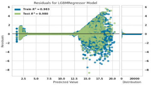
Figure 7. Residual graph of actual and predicted wind speed
Figure 8. Wind speed forecast error diagram
Figure 9. Wind speed training and validation curve
Figure 10. Predicted and actual wind speed chart for 1 day
Finally, the diagram of model learning in power prediction is shown in Figure 5. As is seen, after training 35,000 samples, the difference between the training curve and the validation curve was about 0.001, the training accuracy reached 0.999, and the validation accuracy reached 0.998, both of which are very suitable values.
Figure 6 shows the sum of the powers measured and predicted by the proposed algorithm once a month. In addition to providing the power of our proposed algorithm, this chart can be used in power generation planning to meet power needs. Supposing that the wind farm pro- duction capacity is not enough, in that case, help can be obtained from other power plants to meet shortages. When extra capacity is available, other power plants reduce their production capacity and transfer the wind turbine production capacity to the main power distribution network.
In Figure 7, the green dots show the difference between the actual value and the value predicted by the LightGBM algorithm on the test data, and the blue dots show the difference between the actual value and the value predicted by the LightGBM algorithm on the training data.
The results showed that the error range of the LightGBM algorithm in predicting the wind speed is between -9 and 6 m/s. Also, the maximum error range is between -2 and 2 m/s; these values show that most of the prediction errors are between -2 and 2 m/s, which means that this algorithm either predicts the wind speed by 2 m/s more than the actual value, or it predicts the wind speed -2 m/s less than the actual value.
Figure 8 shows the amount of error between the actual wind speed and the predicted wind speed by the proposed algorithm. In this figure, the actual wind speed values are placed on the x-axis and the predicted wind speeds are placed on the y-axis, and the error between the actual and predicted speeds are shown. To analyze the performance of the algorithm, two lines of best fit and identity are used, so that the more the lines of best fit and identity match each other, the better the algorithm works.
The results show that the wind speed range of this SCADA system is between 0 and 25 m/s, and the proposed algorithm does not have much error because there is a slight error in predicting wind speeds between 2-3 m/s and 13-20 m/s, and the lines of best fit and identity do not completely coincide in these intervals.
Finally, the model learning diagram for predicting wind speed is shown in Figure 9. As is seen, after training more than 35,000 samples, the difference between the training curve and the validation curve was about 0.002, the training accuracy reached 0.983, and the validation accuracy reached 0.980, both of which are acceptable due to the volatile nature of wind speed.
Figure 10 shows the measured wind speed and the obtained forecasts for 1 day. In this figure, every 10 minutes during 24 hours a day, the WS anticipated by the LightGBM algorithm and the actual amount of wind speeds are recorded and collected together in one illustration. As it turns out, the wind speed is well predicted. Therefore, there should be no concern about the nature of wind energy fluctuations, and the application of the adopted model can be the most critical factor in generating wind farm electricity. Wind means predicting wind speed, so turbine production capacity can undoubtedly be predicted by correctly predicting wind speed. It is possible to measure the performance of algorithms using the formulas below:
$\begin{gathered}M S E=\frac{1}{m} \sum_{i=1}^m\left(T_i-\hat{T}_i\right)^2 \\ R M S E=\sqrt{\frac{1}{m} \sum_{i=1}^m} \\ M A E=\frac{\sum_{i=1}^m\left|T_i-\hat{T}_i\right|}{m} \\ M A P E=\left|\frac{1}{m} \sum_{t=1}^m \frac{T_i-\hat{T}_i}{T_i}\right|\end{gathered}$ (8)
where Tiare the actual values, $\hat{T}_i$ are the predicted values, and m is the number of test data for 1 month.
According to the results given in Table 1, the wind speed, which is the essential factor in power generation in wind farms, was well predicted, with a very acceptable value of 0.32 for the criterion of mean squared error and 0.56 for squared mean squared error. Finally, an 0.21 error was achieved for the absolute mean value. It may be asked why, despite the value of 0.56 for the RMSE evaluation criterion, the wind speed graphs were not more accurately predicted and did not fit completely with the actual ones. There is a slight difference in the actual and predicted wind speeds.
In predicting power, the evaluation criteria R2, MSE, RMSE, MAE, and time for power test data with a LightGBM are listed in Table 2.
Table 1. Evaluation criteria R2, MSE, RMSE, MAE, and time for wind speed test data with LightGBM on test data (1 month)
|
Model |
MSE |
RMSE |
MAE |
R2 |
Time (s) |
|
LightGBM |
0.32 |
0.56 |
0.21 |
0.98 |
25 |
Table 2. Evaluation criteria R2, MSE, RMSE, MAE, and time for power test data with Light- GBM on test data (1 month)
|
Model |
MSE |
RMSE |
MAE |
R2 |
Time (s) |
|
LightGBM |
18.2 |
4.27 |
2.71 |
1 |
90 |
Table 3 shows the evaluation criterion R2, MSE, RMSE, MAE, and time for wind speed test data with other algorithms. By comparing the results of Table 3 and Table 1, the superiority of the results of the proposed LightGBM algorithm over the Extra Trees, AdaBoost, KNN, and Ridge algorithms in predicting wind speed is evident.
Table 4 shows the evaluation criteria R2, MSE, RMSE, MAE, and time for power test data with other algorithms. By comparing the results of Table 4 and Table 2, the superiority of the results of the proposed LightGBM algorithm over the Extra Trees, AdaBoost, KNN, and Ridge algorithms in predicting the wind turbine production power is evident.
Table 3. Evaluation criteria R2, MSE, RMSE, MAE, and time for wind speed test data with other algorithms on test data (1 month)
|
Model |
MSE |
RMSE |
MAE |
R2 |
Time (s) |
|
Extra Trees |
0.4221 |
0.6494 |
0.2326 |
0.9764 |
39.66 |
|
AdaBoost |
0.6589 |
0.8113 |
0.5372 |
0.9632 |
3.35 |
|
KNN |
0.4291 |
0.6546 |
0.2462 |
0.9760 |
0.9 |
|
Ridge |
1.8833 |
1.3719 |
1.0209 |
0.8947 |
0.21 |
Table 4. Evaluation criteria R2, MSE, RMSE, MAE, and time for power test data with other algorithms on test data (1 month)
|
Model |
MSE |
RMSE |
MAE |
R2 |
Time (s) |
|
Extra Trees |
3.8 |
1.86 |
0.291 |
1 |
35.46 |
|
AdaBoost |
5741.4 |
75.57 |
67.02 |
0.9969 |
6.02 |
|
KNN |
51902.1 |
226.65 |
92.65 |
0.9722 |
8.4 |
|
Ridge |
110288 |
331.97 |
222.3370 |
0.9409 |
0.2 |
In this article, a SCADA system for a wind farm [19] was studied. The data of a Turkey farm were recorded every hour for a year. The data included wind direction in degrees, WS in m/s, the energy produced in kW, and air temperature in °Celsius. Using the LightGBM algorithm, the WS was predicted. In less than 1 minute, the value of 0.2503 was obtained for the RMSE criterion. Production capacity was also predicted using the LightGBM and 4.27 RMSE crite- rion was achieved. The present article’s best mean square error for the SCADA system in Turkey was 0.32 m/s, whereas in [18], the most significant result was achieved by the ensem- ble using ML techniques to estimate wind speed (WS), with a mean square error of around 12 m/s. In another study of Malakouti et al. [17], ML algorithms were used to make predictions about the output of a SCADA system; the highest efficiency was achieved by an additional tree, with a mean square error of 297.53 kWh, whereas in this paper, a result of 18.2 kWh was obtained for the SCADA system in Turkey. The mean absolute error in predicting WS for 6 hours by Pearre and Swan [25] was 2 m/s, whereas the greatest reached in this work based on the SCADA system in Turkey was 0.21 m/s.
The data used in the present research can be accessed on: https://www.kaggle.com/datasets/berkerisen/wind-turbine-scada-dataset.
I am grateful to Almighty God who has helped me in all stages of my life. I also thank my mother who has encouraged me in all stages of my life.
[1] Lindenberg, S. (2009). 20% Wind Energy by 2030: Increasing Wind Energy’s Contribution to US Electricity Supply. Darby, PA, USA: Diane Publishing. Report number: DOE/GO-102008-2578 TRN: US200822%%993.
[2] Sabev, E., Trifonov, R., Pavlova, G., Rainova, K. (2021). Cybersecurity analysis of wind farm SCADA systems. In Proceedings of the 2021 International Conference on Information Technologies (InfoTech), pp. 1-5. https://doi.org/10.1109/InfoTech52438.2021.9548589
[3] Xu, C., Chen, D., Han, X., Shen, W., Wang, C., Shi, L. (2017). Study of integrated optimization design of wind farm in complex terrain. Taiyang Neng Xuebao, 38(12): 3368-3375.
[4] Kunakote, T., Sabangban, N., Kumar, S., Tejani, G.G., Panagant, N., Pholdee, N., Bureerat, S., Yildiz, A.R. (2022). Comparative performance of twelve metaheuristics for wind farm layout optimization. Archives of Computational Methods in Engineering, 29: 717-730. https://doi.org/10.1007/s11831-021-09586-7
[5] Al-Deen, K.A.N., Hussain, H.A. (2021). Review of DC offshore wind farm topologies. In 2021 IEEE Energy Conversion Congress and Exposition (ECCE), pp. 53-60. https://doi.org/10.1109/ECCE47101.2021.9595070
[6] Liu, H., Chen, C., Lv, X., Wu, X., Liu, M. (2019). Deterministic wind energy forecasting: A review of intelligent predictors and auxiliary methods. Energy Conversion and Management, 195: 328-345. https://doi.org/10.1016/j.enconman.2019.05.020
[7] Zendehboudi, A., Baseer, M.A., Saidur, R. (2018). Application of support vector machine models for forecasting solar and wind energy resources: A review. Journal of Cleaner Production, 199: 272-285. https://doi.org/10.1016/j.jclepro.2018.07.164
[8] Bermejo, J.F., Fernández, J.F.G., Polo, F.O., Márquez, A.C. (2019). A review of the use of artificial neural network models for energy and reliability prediction. A study of the solar PV, hydraulic and wind energy sources. Applied Sciences, 9(9): 1844. https://doi.org/10.3390/app9091844
[9] Wang, Y., Yu, Y., Cao, S., Zhang, X., Gao, S. (2020). A review of applications of artificial intelligent algorithms in wind farms. Artificial Intelligence Review, 53: 3447-3500. https://doi.org/10.1007/s10462-019-09768-7
[10] Márquez, F.P.G., Gonzalo, A.P. (2021). A comprehensive review of artificial intelligence and wind energy. Archives of Computational Methods in Engineering, 29: 1-24. https://doi.org/10.1007/s11831-021-09678-4
[11] Rajagopalan, S., Santoso, S. (2009). Wind power forecasting and error analysis using the autoregressive moving average modeling. In 2009 IEEE Power & Energy Society General Meeting, pp. 1-6. https://doi.org/10.1109/PES.2009.5276019
[12] Singh, P.K., Singh, N., Negi, R. (2019). Wind power forecasting using hybrid ARIMA-ANN technique. In Ambient Communications and Computer Systems: RACCCS-2018, pp. 209-220. https://doi.org/10.1007/978-981-13-5934-7_19
[13] Chen, N., Qian, Z., Nabney, I.T., Meng, X. (2013). Wind power forecasts using Gaussian processes and numerical weather prediction. IEEE Transactions on Power Systems, 29(2): 656-665. https://doi.org/10.1109/tpwrs.2013.2282366
[14] Azimi, R., Ghofrani, M., Ghayekhloo, M. (2016). A hybrid wind power forecasting model based on data mining and wavelets analysis. Energy Conversion and Management, 127: 208-225. https://doi.org/10.1016/j.enconman.2016.09.002
[15] Yang, L., He, M., Zhang, J., Vittal, V. (2015). Support-vector-machine-enhanced markov model for short-term wind power forecast. IEEE Transactions on Sustainable Energy, 6(3): 791-799. https://doi.org/10.1109/TSTE.2015.2406814
[16] Ti, Z., Deng, X.W., Zhang, M. (2021). Artificial Neural Networks based wake model for power prediction of wind farm. Renewable Energy, 172: 618-631. https://doi.org/10.1016/j.renene.2021.03.030
[17] Malakouti, S.M., Ghiasi, A.R., Ghavifekr, A.A., Emami, P. (2022). Predicting wind power generation using machine learning and CNN-LSTM approaches. Wind Engineering, 46(6): 1853-1869.. https://doi.org/10.1177/0309524X221113013
[18] Malakouti, S.M. (2023). Use machine learning algorithms to predict turbine power generation to replace renewable energy with fossil fuels. Energy Exploration & Exploitation, 41(2): 836-857. https://doi.org/10.1177/01445987221138135
[19] https://www.kaggle.com/datasets/berkerisen/wind-turbine-scada-dataset, accessed on Dec. 31, 2022.
[20] Malakouti, S.M., Ghiasi, A.R. (2022). Evaluation of the application of computational model machine learning methods to simulate wind speed in predicting the production capacity of the Swiss Basel wind farm. In 2022 26th International Electrical Power Distribution Conference (EPDC), pp. 31-36. https://doi.org/10.1109/EPDC56235.2022.9817304
[21] Malakouti, S.M., Ghiasi, A.R., Ghavifekr, A.A. (2022). AERO2022-flying danger reduction for quadcopters by using machine learning to estimate current, voltage, and flight area. e-Prime-Advances in Electrical Engineering, Electronics and Energy, 8: 100084. https://doi.org/10.1109/EPDC56235.2022.9817304
[22] Malakouti, S.M. (2023). Utilizing time series data from 1961 to 2019 recorded around the world and machine learning to create a Global Temperature Change Prediction Model. Case Studies in Chemical and Environmental Engineering, 7: 100312. https://https://doi.org/10.1016/j.cscee.2023.100312
[23] Malakouti, S. M. (2023). Estimating the output power and wind speed with ML methods: A case study in Texas. Case Studies in Chemical and Environmental Engineering, 100324. https://doi.org/10.1016/j.cscee.2023.100324
[24] Malakouti, S.M. (2022). Prostate cancer recognition: Using the random forest technique and other Ml techniques. Chemotherapy: Open Access, 10(6): 2022. https://doi.org/10.35248/2167-7700.22.10.170
[25] Pearre, N.S., Swan, L.G. (2018). Statistical approach for improved wind speed forecasting for wind power production. Sustainable Energy Technologies and Assessments, 27: 180-191. https://doi.org/10.1016/j.seta.2018.04.010