Raveena Selvanarayanan![]() | Surendran Rajandran*
| Surendran Rajandran*![]() | Youseef Alotaibi
| Youseef Alotaibi![]()
© 2023 IIETA. This article is published by IIETA and is licensed under the CC BY 4.0 license (http://creativecommons.org/licenses/by/4.0/).
OPEN ACCESS
Numerous coffee devotees believe that the coffee smell plays a vital role in the coffee-drinking insight, complementing the taste and enhancing delight. In the traditional strategy, aroma patterns and profiles are observed by extensive investigation of human olfaction. However, the outcome tends to be imprecise. Tackling the difficulties encountered in distinct scent profiles linked to various coffee bean varieties, including Arabica, Robusta, Monsoon Malabar, Chikmagalur, and Coorg coffee, as well as diverse roasting techniques, through the utilization of Electronic Nose Applications for the investigation of coffee aromas. The suggested methodology employs e-nose technology utilizing conducting polymer sensors to detect aroma volatile chemicals found in coffee, including furaneol, 2-methylisoborneol, and 3-methylindole. The e-nose olfactory characteristics of coffee beans at various stages of roasting are systematically examined and discernible patterns are duly identified. The average intensity of the coffee aroma perceived at a distance of 10 centimeters was rated as 3.9 on a scale of 5. The observed standard deviation of coffee aroma intensity at a distance of 10 centimeters was determined to be 3.8 on a scale of 5. The p-value associated with the disparity in average fragrance scores was determined to be 0.05.
electronic-nose, coffee quality, hierarchical agglomerative clustering, coffee disease detection, volatile compounds, gas-chromatography, mass spectrometry, machine learning techniques
With rising global consumption, coffee has become one of the world's most popular beverages. Coffee companies are focusing on improving quality and adopting various forecasting approaches in response to rising demand. Coffee fanatics all across the world admire Indian coffee for its rich, diverse quality. In India, coffee has a long and rich history accomplishing way back to the 16th century. It is said that Baba Budan, a Sufi saint, brought seven coffee beans from Yemen and planted them in the hills of Chikmagalur, in the Indian state of Karnataka. The coffee plant expanded rapidly over the country after its seeds were germinated in the Western Ghats' cool, humid climate. Coffee cultivation had become an important sector of commerce in India by the 18th century, especially in the southern regions of Karnataka, Kerala, and Tamil Nadu. Initially, Indian coffee was raised mostly by small-scale farmers and sold in neighborhood markets [1]. To expand output, the British constructed enormous coffee plantations in the highlands of southern India, employing forced labor and improved methods of farming techniques. By the turn of the twentieth century, India had emerged to become one of the world's most important coffee producers, with shipments to Europe and other parts of the world. This distinctive flavor profile of Indian coffee was impacted by the country's diverse terrain and climate. Today, India continues to be a major coffee grower, contributing to an estimated 3% of global coffee production. Arabica and Robusta coffee beans have unique scent characteristics that help distinguish them as indicated in Table 1. One such technique involves the use of Electronic Nose Applications (e-noses), which can detect and analyze the aroma profiles of coffee samples [2]. Conductor polymer sensors detect the presence of volatile organic compounds in coffee aroma and detect the freshness of the coffee.
Table 1. History of coffee and its flavor
|
Type |
History |
Grown |
Flavor |
|
Arabica coffee |
17th century |
Hills of Karnataka, Tamil Nadu, and Kerala |
The mild, fruity flavor is often used in blends |
|
Robusta coffee |
20th century |
Southern states of Karnataka, Kerala, and Tamil Nadu |
Strong, bold flavor and higher caffeine content |
|
Monsoon Malabar coffee |
19th century |
Malabar Coast of Karnataka, Kerala, and the Nilgiris mountains of Tamil Nadu |
Strong spicy, smoky, and earthy notes or malty sweetness. |
|
Chikmagalur coffee |
9th century |
Chikmagalur district of Karnataka |
Bright, floral aroma and rich, fruity flavor with notes of chocolate and caramel. |
|
Coorg coffee |
17th century |
Coorg region of Karnataka |
Fruit and a hint of acidity |
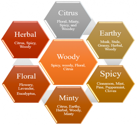
The human brain consists of five senses olfactory which uses most of the brain area in our daily lives The Gustatory Cortex is for taste, the Auditory Cortex is for hearing, the Visual Cortex is for seeing, and the Olfactory Cortex is for Smell. There are two ways of smell detection Orthonasal smell and Retronasal smell. An Electronic Nose Application is a device that can detect and identify different odors or smells. Electronic Nose Applications analyze the volatile compounds in a sample and compare them to a database of known smells. In the case of coffee, an Electronic Nose Application could be used to identify different varieties of coffee based on their aroma. The Electronic Nose Application recognizes harmful or deadly gases that human sniffers cannot. An Electronic Nose Application is equipment that detects and recognizes various odors or aromas [3]. Electronic Nose Applications analyze the volatile substances in a sample and compare them to a database of recognized odors as indicated in Figure 1. In the instance of coffee, an Electronic Nose Application might be used to distinguish between various types based on their smells.
Figure 1. Coffee smell and categories
A possible approach to building an Electronic Nose Application for detecting coffee categories is training it on the distinct volatile substances in each variety. Coffee aroma is composed of a variety of volatile molecules that add to its distinct and complex fragrance, including aldehydes, ketones, pyrazine, thiols, esters, and others. Electronic Nose Applications are assembled from a network of sensors designed to detect a wide variety of chemicals. The Electronic Nose Application works by analyzing the unique pattern of signals it generates in response to a sample used to identify the substances it contains. E-nose (Electronic Nose Application) systems commonly use electronic signal processing. It's a term for the methods by which the electrical signals generated by the e-nose sensors are extracted and analyzed. E-nose sensors react to volatile organic compounds (VOCs) in a coffee sample by sending out complex and often audibly distracting electronic signals [4]. Electronic signal processing techniques are used to eliminate noise from sensor data and retrieve pertinent data. Hierarchical clustering, formerly referred to as cluster analysis with hierarchical structure or HCA is another unsupervised Machine Learning Techniques approach for clustering unlabeled datasets [5]. The construction of a cluster hierarchy in the outline of a tree is referred to as hierarchical clustering, and this tree-shaped structure is known as the dendrogram. K-means and hierarchical clustering results can appear identical at times, however, could vary depending on how they work [6]. Agglomerative (bottom-up) and Divisive (top-down) techniques are used for hierarchical clustering.
A dendrogram, which is a tree-like envision generated by hierarchical clustering, displays the hierarchical relationships between groupings. Individual data points are at the bottom of the dendrogram, while the largest clusters, which contain all of the data points, are at the top. The dendrogram can be cut at different heights to yield varying numbers of clusters [7]. Section 2 discusses the related work of the existing model in detecting and categorizing coffee aromas.
Zhang and Deng [8] proposed employing an Electronic Nose Application to identify odors inspired by extreme learning machines. The self-expression model (SEM) and the extreme learning machine (ELM) are two real-time verified methods for detecting aberrant odor 96 target samples and 24 aberrant samples were used in training and testing. The scents of perfume, flowery water, and fruits were used in Real-Time Abnormal Odor without Target Odor. The intended odor recognition rate is 90.67%, whereas the anomalous odor recognition rate is 91.67%. Fang et al. [9] proposed an olfactory algorithm in all features based smart Electronic Nose Application. The technique mixes one-dimensional convolutional and recurrent neural networks. Deep-learning-enabled sensor array code signs and recognition algorithms may aid in meeting the growing need for a large number of highly specialized gas sensors. Deep-learning-enabled e-nose code sign paradigm that automatically learns target-specific features and optimizes sensor materials and sampling procedures iteratively.
Liu et al. [10] proposed wine properties detection using a MOS sensor and Machine Learning Techniques algorithm using an Electronic Nose Application. Odor detection includes the area of production, fermentation process, vintage years, and variants of four groups of test runs, the extreme gradient boosting (Xgboost), support vector machine (SVM), random forest (RF), and backpropagation neural network (BPNN) datasets were utilized, and the results were achieved 94% by analyzing wine properties for 450 in 6 matrices, 600 in 6 matrices, 450 in 6 matrices, or 600 in 6 matrices, correspondingly. Tan and Xu proposed a review of food quality with related properties for e-nose and e-tongue determinations. Feature extraction and classification used ANN and CNN based on the Electronic Nose Application. A coffee sample size is type typically and was collected and tested for training and validation [11].
Mu et al. [12] developed Machine Learning Techniques and algorithms for detecting milk sources and estimating milk quality. Milk fats and proteins are enhanced with an estimated accuracy of 95% using Dairy Herd Improvement (DHI) analytical data that collects data on dairy cows, including their milk production, health, and reproduction, and a five-fold cross-validation technique dividing the data into five-fold, and then training the model on four of the folds and testing it on the remaining fold. This process is repeated five times, and the results from the five tests are averaged to get an estimate of the model's performance based on milk odor features using an Electronic Nose Application. Xu et al. [13] proposed an approach for psychiatric symptoms and volatile organic compounds in trans-diagnostic samples using an Electronic Nose Application. 1200 participant’s characteristics were collected based on age, sex, smoking status, BMI, depression PHQ-90, Anxiety OASISd, Addiction DAST-10e, Race Ethnicity, and Education datasets were collected and processed using Machine Learning Techniques and data analysis. Hayasaka et al. [14] proposed a Machine Learning Techniques-based strategy based on three types of gas water (H2O), methanol (MeOH), and ethanol (MtOH) in a single graphene FET using e-nose. MFC1 and MFC2 controlled the background R.H., while MFC3 controlled the target gas concentration. Controlling overfitting and performing cross-validation tests ensured accuracy.
Dadi et al. [15] suggested a sensor array reduction for detecting odor utilizing e-nose. The cross-validation approach is used to calculate performance using the usual leave-one-group-out and group shuffling methods. The increased odor recognition power of e-noses obtained 95% performance from training and cross-validation. Ye et al. [16] developed recent developments towards smart Electronic Nose Applications, a Machine Learning Techniques approach. Advanced Machine Learning Techniques and methodologies are required for the e-nose to improve its performance and capabilities in a variety of applications, including robotics, food engineering, environmental monitoring, and medical diagnosis. Using Machine Learning Techniques and algorithms improved both qualitative and quantitative analysis outcomes. A Machine Learning Techniques-based prediction approach for detecting coffee quality from green to roasted coffee beans was proposed by Suarez-Peña et al. [17]. The neural network algorithm is compared to support vector classification. The findings of the analysis of green coffee bean attributes were predicted as high or low with a classification shoehorn accuracy of 81% using 10-fold stratified cross-validation procedures.
Harsono et al. [18] advocated employing e-nose in Machine Learning Techniques to recognize odors in original Arabica civet coffee. This study focuses on a blend of Arabica civet coffee and Robusta coffee, which results in nine different mixing combinations. A statistical computation would be determined to obtain parameter statistics. Furthermore, the classification approach used in this work is intended to discriminate between original Arabica civet coffee and original Robusta coffee. The KNN technique yields the best results, with an accuracy rating of 97.7% for nine classes as indicated in Table 2.
Caporaso et al. [19] suggested a hyperspectral imaging-based prediction method for single-roasted coffee beans. The current work used hyperspectral imaging (1000-2500 nm) to predict volatile chemicals in single roasted coffee beans, as assessed by Solid Phase Micro Extraction-Gas Chromatography-Mass Spectrometry and Gas Chromatography Olfactometry. Individual beans can be separated, resulting in batches of coffee with varying volatile flavor element combinations.
Hendrawan et al. [20] and colleagues suggested utilizing Deep Learning approaches to detect and categorize purity levels in luwak coffee green beans. The study sought to detect and classify the purity of Luwak coffee green beans into four categories: deficient (0-25%), low (25-50%), medium (50-75%), and high (75-100%). Based on the training and validation data, GoogleNet was recognized as the best CNN model with optimizer type Adam and a learning rate of 0.0001, with an accuracy of 89.65%. García et al. [21] proposed using computer vision to detect quality and flaws in green coffee beans. Color, morphology, shape, and size are all critical indicators of high-quality beans. To determine the quality of coffee beans, the k-nearest neighbor approach was applied. AI-based vision technique for choosing high-quality coffee beans to reduce production time and increase quality control. Angeloni et al. [22] proposed an expresso coffee aroma profile based on its properties and odorants. The odor of coffee arabica and canephora is evaluated using volatile analysis and chemical attributes to determine the granulomere of the coffee particles and the brew ratio, which can modify the aroma profile of the beverage. The optimized extraction procedure may enable greener EC preparation and consumption by using less coffee powder to generate the same amazing output.
Table 2. Summary of coffee variety and aroma
|
Reference |
Contributor |
Method |
Samples |
Accuracy |
|
[8] |
Zhang and Deng |
Self-expression and Extreme Machine Learning |
96 samples |
91.67% |
|
[10] |
Liu et al. |
MOS Sensor |
1200 samples |
94% |
|
[11] |
Tan and Xu |
ANN and CNN-based e-nose |
180 samples |
91% |
|
[12] |
Mu et al. |
Milk Odor Features Based e-nose |
DHI Samples |
95% |
|
[13] |
Xu et al. |
Machine Learning Techniques and Data Analysis |
1200 samples |
95% |
|
[15] |
Dadi et al. |
Cross-validation method |
650 samples |
95% |
|
[17] |
Suarez-Peña et al. |
Support Vector Machine |
597 samples |
81% |
|
[18] |
Harsono et al. |
KNN |
Nine mixing combination |
97.7% |
|
[19] |
Caporaso et al. |
Chromatography-Mass Spectrometry and Gas Chromatography Olfactometry |
Solid Phase Micro Extraction |
1000-2500 nm |
|
[20] |
Hendrawan et al. |
Deep Learning approaches |
75-100% Coffee Sample |
89.65% |
|
[23] |
Thanarajan et al. |
e-nose |
Odor Categorization |
97.1% |
|
[24] |
Raveena and Surendran |
Deep CNN ResNet50 |
459 samples |
99.01% |
Thanarajan et al. [23] proposed using an Electronic Nose Application to control coffee output quality by odor categorization. Instant coffee samples are collected and analyzed depending on temperature, concentration, and brand, achieving 97.1% overall odor uniqueness. Raveena and Surendran [24] proposed using ResNet50 to classify coffee cherries. Six coffee stages are used for categorizing coffee cherries depending on coffee type and color variation. Using Deep CNN models, the author achieved 99.01% accuracy. Lee et al. [25] proposed an artificial intelligence-based coffee aroma recognition-based fingerprint extraction method. Various fragrances of freshly roasted coffee were collected, and performance was calculated based on individual coffee aroma signatures of authentic quality. Dewangan et al. [26] developed a smell detection model based on Machine Learning Techniques code-based methods. The Chi-square feature extraction technique was used to pick the most significant features in each dataset. The Long-method dataset with the various selected sets of metrics produced the most accuracy (100%) for all five methods; however, the Max voting method produced the lowest accuracy (91.45%) for the Feature-envy dataset with the specified twelve sets of metrics. Zhang et al. [27] suggested a data preprocessing strategy based on polynomial curve fitting (PCF), locally weighted regression (LWR), wavelet package correlation filter (WPCF), and mean filter (MF) for recognizing and detecting coffee odor. The well-known Support Vector Machine (SVM) classifier has a classification accuracy of 96.23%.
Gonzalez Viejo et al. [28] proposed the intensity of coffee aroma profile using an integrated electronic nose at a low cost. Aromatic chemicals in coffee and their representation in a principal component analysis. Overall 270 datasets were trained and validated to evaluate the Performance was assessed based on mean squared error (MSE). Tanveer et al. [29] proposed a Green requirement engineering for mobile application development based on IoT for gathering required mobile challenges. Section 3 discusses the Materials and Methods in the roasting process, and working of Electronic Nose application detection for coffee aromas.
Electronic Nose Application uses conducting polymer sensors which have 12 sensor arrays to detect the VOCs in coffee aroma. Polyaniline (PANI) sensors made from polyaniline. PANI sensors are sensitive to a wide range of VOCs, and they can be used to detect the aroma of coffee, ten samples of Arabica coffee, twelve samples of Robusta coffee, seven samples of Monsoon Malabar coffee, five samples of Chikmagalur coffee, and eight samples of Coorg coffee were examined. Observed data is imported to a CSV file processed for a data science library, such as Pandas. Checked for missing values which can affect the missing values using the clustering algorithm. Data should then be normalized and features should be scaled so that they have a similar range. Model performance is measured using internal and external measurements.
3.1 System architecture and execution
High to High roast can bring the Expresso flavor of Italian and French coffee characteristics, and Medium dark to Medium dark roast can bring the Dark and full city flavor of coffee characteristics. Medium to Medium roast can bring the Dark and Rich flavor of coffee characteristic.
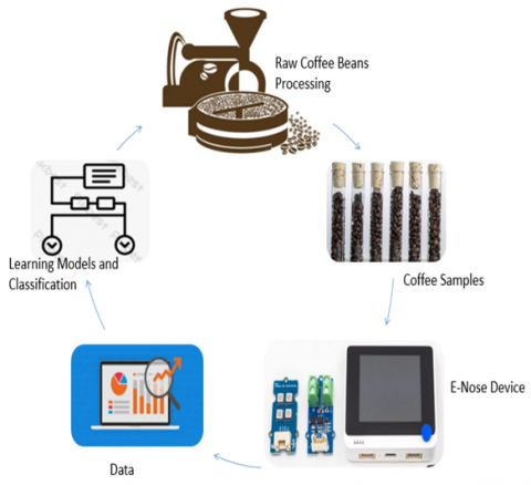
The coffee having a light-to-light roast might have a cinnamon flavor. The venture began with processing green coffee beans under continual roasting conditions, ranging from unflavoured green beans to those with a distinct smell. Researchers then collected various pieces of freshly roasted coffee beans. They stored them in the device's concentrate container to capture the resulting coffee fragrance after a sufficient period of the discharge method. After that, the aromatic gas was transported to the e-nose device, where it interacted with sensors. The sensor data that emerged was then collected and preprocessed so that the procedure could be applied to as much relevant information as possible. The extracted fragrance dataset was utilized to train the machine-learning models that were chosen for the recognition task as illustrated in Figure 2.
Figure 2. System architecture
3.2 Coffee roasting techniques
Water covers 7 to 11% of the weight of a green coffee bean from various varieties such as Arabica, Indiana, Keny’s, S.795, Cauvery, and Chandragiri and is evenly distributed throughout the grain structure. Coffee beans cannot turn brown if there is water in the coffee cherry, hence the Stage 1 drying process is required. After the water in the coffee beans has evaporated, the first browning reaction occurs. The beans remain hard and substantial, with a faint aroma of Indian rice and a hint of bread flavor. The coffee beans will grow in size, and the silk cover will begin to peel away. Stage 2 is when the wind blows into the roasting cage and removes the silk skin from the coffee beans, which are then safely gathered to avoid burning. The initial break is stage 3 caused by the evaporation of Carbon dioxide gas and water vapour. The roasting process continues for flavor and aroma development, and the sourness will rapidly subside at this stage 4 [30]. After the second burst of roasting, the oil will begin to trickle over the surface of the coffee beans, and ordinary coffee flavor will develop.
3.3 Experimental process
The Experimental process is broadly divided into four stages. Stage one coffee is roasted and processed to the final stage. Stage two roasted samples as shown in Table 1, odors from processed samples are collected depending on several characteristics such as Arabica, Indiana, Keny's, S.795, Cauvery, and Chandragiri. Some measures are made based on VOC by comparing them to the aroma of newly roasted coffee placed in a chamber for the measurement process. The researchers next experimented with freshly roasted ground coffee, taking samples and roasting green coffee beans in a lab-specific machine. Once the coffee had been suitably roasted, it was crushed and combined with hot water, which facilitated the measurement process because liquid coffee produced more volatiles, as seen in Table 2. Sample testing can be done by simply exposing the Electronic Nose Application to the coffee aroma in the liquid samples or air. Once the sample is gathered, the Electronic Nose Application employs conducting polymer sensors to determine the chemical makeup of the coffee aroma. Each sensor is tailored to detect a single chemical component or combination of chemicals. The sensors' data are then analyzed using algorithms to determine the distinct pattern of signals linked with the coffee fragrance. To identify the coffee odor, this pattern is compared to a database of known patterns. Depending on the application, the output of the Electronic Nose Application can be shown in a variety of ways. In a quality control predicament, the output might simply be a success or failure indicator depending on whether or not the coffee scent fits the required requirements.
A complete examination of the chemical content of the coffee smell may be generated in a controlled laboratory setting. High quantities of 2-Phenylethanol and Citric acid in Arabica may imply a more flowery and acidic scent, but high amounts of Furaneol may indicate a sweeter, caramel-like aroma. High quantities of 3-methyl butanal and 2-methyl propanol in Robusta may suggest a nuttier and earthy scent, whilst high amounts of 2-Ethyl-3, 5-dimethyl pyrazine may indicate a smoky and somewhat bitter aroma. Greater quantities of 2-Methylbutanal in Keny's could point to a nutty and caramel-like scent, even with greater levels of 2-Furfurylthiol may indicate a more intense roasted aroma. In S.795, higher 2-methylbutanal levels may imply a nutty and caramel-like scent, whilst higher 2-furfurylthiol levels may indicate a stronger roasted aroma. Greater quantities of 2-methylbutanal in Chandragiri may imply a nutty, caramel-like scent, whilst greater levels of 2-Furfurylthiol may indicate a more determined roasted aroma. Representative coffee samples are selected based on variety and quality parameters, such as origin, roast level, and processing method. Once the samples have been selected, they are prepared for testing using standard procedures such as grinding and weighing.
3.4 Electronic nose application
Subsequently receiving coffee specimens and Electronic Nose Application will examine the aroma profile of the coffee by identifying and measuring the volatile organic compounds (VOCs) contained in the sample, as indicated in Table 3. These VOCs contribute to the coffee's distinct odor and flavor qualities, which the Electronic Nose Application can deeply analyze by the variety of chemical sensors, each of which is programmed to respond to a certain volatile organic compound (VOC). Conducting polymer sensors, conducting polymers, and carbon nanotubes are some of the materials that can be used to make these sensors. Each sensor's response is recorded and analyzed to determine the individual odors present in the sample. The Electronic Nose Application combines a variety of chemical sensors to detect and quantify the various volatile organic compounds (VOC) in coffee samples. It then compares the measured VOC patterns to a collection of known aroma profiles to determine the coffee's variety, age, and other features. Based on this study, the Electronic Nose Application can provide an exhaustive sensory rating of the coffee, including smell intensity, complexity, and balance. Coffee producers may utilize the aforementioned data to improve the quality and consistency of their coffee, allowing coffee enthusiasts to better understand and enjoy the coffee they are experiencing.
Table 3. Characteristics of coffee aroma
|
Coffee Type |
Chemical Compound |
Unique Aroma |
Method |
|
Arabica Coffee |
2-Phenylethanol 2-Methylbutanal 2, 3-Butanedion 2,5-Dimethyl-4-hydroxy 3(2H)-furanone (Furaneol) |
Floral Aroma Bright and Acidic Aroma Sweet Aroma Buttery or Creamy Caramel |
(GC-MS) Gas Chromatography-Mass Spectrometry |
|
Robusta Coffee |
3-Methylbutanal 2-Methylpropanal 2-Ethyl-3, 2-Ethyl-3,5-dime 2-Methoxyphenol (Guaiacol) 2-Isopropyl-3 methoxypyrazine |
Nutty Aroma Earthy Aroma Smoky and Bitter Aroma Woody and Spicy Aroma Strong and Pungent Aroma |
(GC-MS) Gas chromatography-Mass Spectrometry |
|
Keny’s Coffee |
2-Methylbutanal 2-Furfurylthiol 2-Isobutyl-3 -methoxypyrazine Dimethyl sulfide |
Nutty and Caramel Aroma Roasted and Burnt Aroma Green, Herbal, and Vegetative Aroma Sulfurous Aroma |
Volatile Organic Compounds |
|
S.795 Coffee |
2-Methylbutanal 2-Furfurylthiol 2-Isobutyl-3 Methoxypyrazine Guaiacol |
Nutty and Caramel Aroma Roasted and Burnt Aroma Green, Herbal, and Vegetative Aroma Sulfurous Aroma |
(GC-MS) Gas chromatography-Mass Spectrometry |
|
Carvery Coffee |
2-Methylbutanal 2-Furfurylthiol 2-Isobutyl-3 Methoxypyrazine Guaiacol |
Nutty and Caramel Aroma Roasted and Burnt Aroma Green, Herbal, and Vegetative Aroma Sulfurous Aroma |
((GC-MS) Gas chromatography-Mass Spectrometry |
|
Chandragiri Coffee |
2-Phenylethanol 2-Methylbutanal 2-Furfurylthiol 2-Isobutyl-3 -methoxypyrazine Guaiacol |
Roasted and Burnt Aroma Green, Herbal and Vegetative Aroma Sulfurous Aroma |
(GC-MS) Gas- Chromatography-Mass Spectrometry |
3.5 Electronic signal processing
E-signal processing is a technique used for processing and analyzing the signal generated by an e-nose sensor using VOC present in coffee samples. The quantity and variation in volatile organic compounds (VOCs) in Arabica, Keny’s and Robusta coffee samples might vary based on several parameters, including coffee bean variety, origin, processing methods, roast degree, and storage circumstances. Some common VOC found in coffee are Aldehydes: The concentrations can range from a few parts per billion (ppb) to a few parts per million (ppm) depending on the particular aldehyde molecule. Pyrazines: Concentrations can range from a few parts per billion (ppb) to a few parts per trillion (ppt), with roasted and nutty pyrazines standing out. Concentrations of ketones can range from a few ppb to a few ppm, with components like diacetyl and acetoin adding to buttery and creamy aromas.
3.6 Hierarchical agglomerative clustering algorithm
Hierarchical agglomerative clustering is a clustering algorithm that clusters comparable data points together based on their pairwise distances. It is a bottom-up strategy that begins with each data point as a separate cluster and then merges the closest clusters iteratively until a stopping requirement is reached. The similarity metric is the input parameter for hierarchical clustering. It quantifies the proximity between two data points. There are many different similarity metrics available, such as the Euclidean distance. The linkage method is used to merge clusters. There are many different linkage methods available, such as the complete linkage method. The number of clusters desired number of clusters that the algorithm will output. As a result, a hierarchical cluster structure is formed represented as a tree-like structure known as a dendrogram. The process of hierarchical agglomerative clustering.
Steps involved in Hierarchical agglomerative clustering:
Step 1: Initialization: Each data point is created and assigned to its cluster.
I. The hierarchical_Agglomerative_Clustering function initializes the clusters by calling the initialize Clusters function.
II. Each data point is assigned to its cluster.
Step 2: Compute similarity matrix: The similarity between each pair of clusters is computed using a similarity metric such as Euclidean distance.
I. The algorithm enters a loop that continues until only one cluster is left.
II. Inside the loop, the compute_Similarity-Matrix function is called to calculate the similarity between each pair of clusters.
Step 3: Merge closest clusters: The closest pair of clusters is identified based on the similarity matrix and merged to form a new cluster.
I. The Find_Closest-Clusters function is called to find the closest pair of clusters based on the similarity matrix.
II. The Merge_Clusters function is called to merge the closest pair of clusters into a new cluster.
Step 4: Update similarity matrix: The similarity matrix is updated to reflect the similarity between the new and remaining clusters.
Step 5: Repeat steps 3 and 4 until all data points belong to a single cluster and return to the final cluster. Section 4 discusses the Results Analysis based on the Principal Components Analysis for coffee aromas.
To facilitate the advancement of a real-time, high-performance coffee aroma detection system. The experimental setup utilized in this study involved the utilization of a gas chromatograph (GC) to separate the volatile compounds present in coffee aroma. Additionally, a mass spectrometer (MS) was employed to identify the different compounds. The entire process was controlled by a computer, which also facilitated the storage and analysis of the acquired data. Furthermore, software specifically designed for data analysis and machine learning Tensor Flow was employed to process the collected data.
4.1 Collection of datasets
Finding specific datasets on coffee odors can be challenging as the availability of such datasets may be limited 415 coffee odor datasets are collected. Coffee odor samples are collected from various coffee factories based on stages of maturity, texture, aroma, and consistency. The dataset is divided according to their aroma flavors Class-A has a Floral Aroma and Sweet Aroma, Class-B has Acidic Aroma, Sulphurus Aroma, Class-C has a Roasted, Burnt Aroma, Class-D has Woody Spicy Aroma, Class-E has an Earthy Woody Aroma, and Class-F has Nutty Caramel Aroma is tested manually in Indian coffee manufacturing to compare and listed the final samples as indicated in Table 4. Used online datasets such as Google Search, Kaggle, and open data platforms. Visited various sensor analysis database institutions and collected aroma-related descriptive analysis. Browsed relevant research papers in search of datasets based on aroma and a variety of aromas.
Table 4. Odor samples for coffee datasets
|
Coffee Odor Samples |
Class A |
Class B |
Class C |
Class D |
Class E |
Class F |
Total Samples |
|
Arabica |
22 |
12 |
07 |
14 |
21 |
33 |
109 |
|
Robusta |
18 |
15 |
09 |
11 |
11 |
21 |
85 |
|
Keny’s |
14 |
19 |
04 |
08 |
02 |
04 |
51 |
|
S.795 |
09 |
14 |
03 |
08 |
15 |
01 |
50 |
|
Carvery |
08 |
18 |
11 |
16 |
22 |
04 |
79 |
|
Chandragiri |
05 |
09 |
02 |
11 |
09 |
12 |
48 |
4.2 Experiments
In our trials, we use Python alongside the Keras and Tensor Flow frameworks in our model. The network was trained on a system with an Intel Core i5-11400 CPU running at 2.60GHz. The research was conducted utilizing an NVIDIA RTX A5000 GPU, a 64-bit operating system, and 16GB of RAM. The specifics are listed in Table 5. For coffee roasting and grinding blade grinder and drum roaster are used.
Table 5. Experiment required
|
Equipment Details |
Parameters |
|
Blade Grinder |
Model NO-J-235C, Capacity 455mm/18inch |
|
Drum Roaster |
0.25-2HP, 25kg |
|
Electronic Nose Application |
FS7002-B, Sensing Range 0-5m/s, gas, |
|
System Type |
Windows 10, 64bit |
|
CPU, GPU |
Intel Core i9-12900K, AMD Ryzen 9 5950X |
|
Library |
Tens flow |
|
Creation Tool |
Python 3.10.1 |
4.3 Coffee odor-processing
The preprocessing technique improves the quality of information acquired via electronic signal processing. Noise, drift, and undesired abnormalities may be present in signals. Signal processing methods such as amplification and filtering are used to boost signal quality. Filtering techniques (such as low-pass, high-pass, and band-pass filters) can remove noise or undesired frequency components, while amplification helps to improve signal intensity. Baseline correction is used to eliminate any regular drift or offset in sensor signals. This entails estimating and subtracting a baseline value from the signals to bring them all to the same reference level. Calibration is required to ensure consistent and dependable performance. The sensors are calibration models, which can then be used to quantify or classify unknown samples. Thiols, which are often found in trace concentrations in the low ppb range, can contribute to sulfur-like or skunky odors. Concentrations of phenols can range from a few ppb to a few ppm, with substances such as Guaiacol contributing to Smokey and phenolic overtones. Fruity esters add to the aroma complexity of the coffee, with concentrations ranging from a few ppb to a few ppm as indicated. Acids: Organic acids such as acetic acid, formic acid, and quinic acid can be found in concentrations ranging from a few ppm to tens of ppm, contributing to the acidity and flavor character of coffee.
4.4 Principal Components Analysis
Principal Component Analysis (PCA) is an approach for reducing dimensionality and its goal is to reduce a high-dimensional dataset to a lower-dimensional space while retaining the most relevant information or patterns in the data. Each major component is a linear combination of the initial variables. The first principal component is responsible for the greatest possible variance in the data, the second for the second largest variance, and further on. Eqs. (1)-(3) show the mean and SD.
μ−j=(1/n)∗Σ(H−ij) (1)
In data standardization, if the variables in the dataset have different scales, it is common practice to standardize them to have zero mean and unit variance. This step ensures that variables with larger scales do not dominate the analysis. To calculate data standardization, mean and variables are observed where H_ij represents the value of the jth variable for the ith observation, n data points.
σj=sqrt((1n−1)∗Σ((Hij−μj)2)) (2)
To calculate data standardization, the standard deviation (σ) for each variable across all the observations. Subtract the mean from each variable value and divide it by the standard deviation to obtain the standardized value for each observation and variable. Assemble the standardized values into an n x m matrix called H. Each column of H represents a standardized variable, and each row represents an observation.
H−ij( standardized )=(H−ij−μ−j)/σ−j (3)
In Covariance Matrix Calculation provides information about the relationship between variables and how they vary by comparing them together. Let H be the standardized data matrix with dimensions n x m, where n is the number of observations and m is the number of variables. Eq. (4) where X^T is the transpose of X
C=(X∧T∗X)/(n−1) (4)
The eigenvectors in Eigen composition represent the amount of variance explained by each principal component, and the eigenvectors in Eigen composition represent the direction of each principal component. The eigenvectors are ranked in principle component selection according to their corresponding eigenvalues. The major components are the eigenvectors with the highest eigenvalues that explain the most variance in the data. The original dataset is projected onto the selected principal components in dimensionality reduction to obtain the lower-dimensional representation. This projection involves taking a dot product between the standardized data and the eigenvector. The projected data matrix Z has dimensions’ n x k and can be computed as, where * denotes matrix multiplication.
Z=X∗ V (5)
4.4.1 Principal Components Analytical Pseudo code
Transformed Data = Dataset ∗V (6)
Mean is the average of all the values in a set of data. It is calculated by adding all the values and dividing by the number of values. Standard deviation is a measure of how spread out the values in a set of data is. It is calculated by taking the square root of the variance. P-value is a probability value that is used to determine statistical significance. It is calculated by comparing the observed results to the expected results under the null hypothesis.
4.5 Model architecture selection
Hierarchical Agglomerative Clustering (HAC) is a bottom-up clustering algorithm that recursively merges data points or clusters to form a hierarchical structure of clusters. After completing the Principal Components Analysis statistical dataset is moved into the initialization process where each data point is set as an individual cluster. Calculate the distance between each pair of clusters using Euclidean distance which is used to calculate the distance between two points (A1, A2) and (B1, B2) in an Euclidean space, S represents distance Eq. (7).
S=sqrt((A2−A1)2+(B2−B1)2+(C2−C1)2) (7)
Figure 3. Working flow of proposed work
To find the two closest merging or linkage criteria merge closest is used. Four closest are compared and used such as Single linkage for calculating the smallest pair of distances, Complete linkage for calculating the maximum smallest pair of distances, Average Linkage for calculating the smallest average pair of distances, and Ward’s linkage. After merging, try to reduce the rise in total within-cluster variation. After merging two clusters, update the distance matrix to reflect the distances that exist between the newly formed cluster and the existing clusters. The distance between the merged cluster and another cluster can be determined via several methodologies, such as the minimum distance, maximum distance, or average distance between their respective members. Repeat the merging and distance matrix updating stages until all data points or clusters are merged into a single cluster or an initial number of clusters is reached. The merging process represents the relationships between clusters at different levels of granularity and is called a Hierarchical cluster tree also called a dendrogram. To determine the desired number of clusters, the dendrogram can be visually analyzed. The final clusters are determined by cutting the dendrogram at a specified height or by a distance criterion as indicated in Figure 3.
4.6 Training and validation
Datasets of coffee aroma are collected based on features and voltaic components. The dataset was preprocessed by cleaning, normalizing, and transforming the aroma features as needed. Based on different aroma level factors such as coffee origin, roast level, and brewing method using Hierarchical Agglomerative Clustering [31, 32]. The dataset is separated into training and validation to fit the Hierarchical Agglomerative Clustering for analyzing coffee aroma and the trained model to make predictions on the validation dataset.
4.6.1 Training set
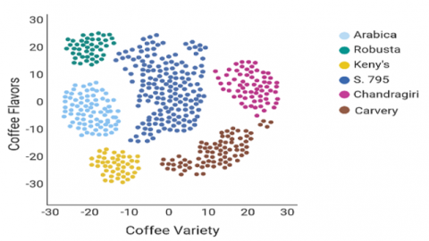
Initially, the data preparation process involves splitting the available coffee aroma 415 samples into a training set, validation set, and test set 291:62:62 ratios. Model initialization involves assigning each data point to its cluster so that each data point is considered a singleton cluster. Firstly, the distance between each pair of data points is calculated using Euclidean distance in each iteration two clusters are merged into a new cluster until all data points are merged. Finally, create a cluster hierarchy that represents the history of merging clusters, allowing for different levels of granularity in the clustering solution. A training loop operates to acquire and train the data to forecast the accurate value for each epoch. Forward propagation is the process of computing output values by moving input data from the input layer to the output layer across the network's layers. The loss calculation function determines the loss value using the expected output and the true labels as input. The loss value represents the algorithm's current performance on the given input. Back propagation calculates the gradient loss concerning the model parameters again loss calculation is done to maintain the data accuracy as indicated in Figure 4.
Figure 4. Coffee variety and flavors
4.6.2 Validation set
The validation set helps monitor and hyper-fine-tune the models and is an intermediate between the training and test sets. Clustering-based validation set has multiple performance evaluation metrics that can be used depending on the specific task and the nature of the data. The measurement of performance can be clustered using External Measurements: Rand Index (RI), Jaccard Coefficient, Calinski-Harabasz Index, Normalized Mutual Information (NMI), and Fowlkes-Mallows index. Internal Measurements: Silhouette Coefficient, Dunn Index, and Davies-Bouldin Index.
Silhouette Coefficient: This metric assesses how well each data point fits within its given cluster compared to others. It has a value between -1 and 1, with higher values indicating stronger clustering. The average distance between one point and all other points in the same class. This score represents the closeness of points in the same cluster. The average distance between a sample and the nearest cluster's other points. This score computes the distance between points in various clusters, where, a (i) represents the intra-clustering distance and b (i) represents the inter-clustering distance.
Silhouette coefficient=b(i)−a(i)/max (8)
Calinski-Harabasz Index: This is a clustering evaluation metric that is used to evaluate the quality of clustering results. It calculates the ratio of between-cluster to within-cluster dispersion. The index attempts to capture cluster compactness and separation, where CH is the Calinski-Harabasz Index. B is the dispersion between clusters. W is the dispersion inside the cluster. The total number of data points is denoted by N. The number of clusters is k.
\mathrm{CH}=(\mathrm{B} / \mathrm{W}) *((\mathrm{~N}-\mathrm{K}) /(\mathrm{k}-1)) (9)
Davies-Bouldin Index: Clustering evaluation metric that calculates the average similarity across clusters by considering intra-cluster and inter-cluster distances. It provides a quantitative evaluation of the clustering results' quality. Where DB represents the Davies-Bouldin Index and k represents the number of clusters. R (i, j) represents the average distance between clusters I and j. The average intra-cluster distance of cluster i is represented by R (j, i).
D B=(1 / k) * \epsilon(\max (R(i, j)+R(i, j))) f (10)
Dunn Index: The ratio of the minimum inter-cluster distance to the maximum intra-cluster distance. The greater the Dunn Index, the superior the clustering result, where min-inter is the shortest distance between any two clusters and max-intra is the shortest distance between any two data points within the same cluster.
Dunn Index = min_inter / max_intra (11)
Normalized Mutual Information (NMI): calculates the normalized mutual information between two sets of labels, such as the predicted cluster labels and the true class labels. It provides a measure of how well the clustering aligns with the true underlying structure of the data where MI is the mutual information between the two label sets, H1 is the entropy of the first label set, and H2 is the entropy of the second label set.
\mathrm{NMI}=(2 * \mathrm{MI}) /(\mathrm{H} 1+\mathrm{H} 2) (12)
Rand Index (RI): Calculates the similarity measure between two data clustering, where w is the number of data points in both clustering that belong to the same cluster (true positives). H is the number of data point pairs that belong to different clusters in both clustering (true negatives). V2 is the total number of data point pairs.
\mathrm{RI}=\frac{\mathrm{w}+\mathrm{h}}{\mathrm{v}^2} (13)
Jaccard Coefficient: The similarity measure quantifies the overlap between two sets, where C denotes the set of data points assigned to a specific cluster by the clustering algorithm. D is a set of data points that belong to a given class or ground truth cluster.
J C=(\mid number of elements in common \mid) /|total number of elements| (14)
Fowlkes-Mallows index (FMI): calculates the measure of similarity between two clustering. It combines precision and recall to evaluate the agreement between the two clustering where TP (True Positives) represents the number of pairs of data points that are in the same cluster in both clustering (agreements). FP (False Positives) represents the number of pairs of data points that are in the same cluster in the clustering result but not in the ground truth clustering. FN (False Negatives) represents the number of pairs of data points that are in the same cluster in the ground truth clustering but not in the clustering result.
\mathrm{FMI}=(\mathrm{TP} / \sqrt{(\mathrm{TP}+\mathrm{FP})} * \sqrt{\mathrm{TP}+\mathrm{FN}}) (15)
The initialize Clusters function creates individual clusters for each data point using Python code.
Function initialize Clusters (data):
Clusters= []
For each data point in data:
cluster=create a cluster (data Point)
Clusters. Append (cluster)
Return clusters
The compute_Similarity-Matrix function computes the similarity between each pair of clusters and stores the values in a similarity matrix using Python code.
Function compute_Similarity-Matrix (clusters)
Similarity matrix=empty matrix of size (num Clusters, num Clusters)
For i=1 to num Clusters
For j I I+1 to num Clusters
Similarity=compute Similarity (clusters [i], clusters [j])
Similarity matrix [i, j] =similarity
Similarity matrix [j, i] =similarity
Return similarity matrix
Function compute_Similarity (cluster1, cluster2)
The find Closest_Clusters function identifies the pair of clusters with the minimum distance in the similarity matrix using Python code.
Function find Closest-Clusters (similarity matrix)
Instance=infinity
Merge Indices= (0, 0)
For i=1 to num clusters
For j=i+1 to num clusters
Similarity matrix [i, j] <instance:
Instance=similarity matrix [i, j]
Merge Indices = (i, j)
Return merge Indices
The merge_Clusters function merges the closest pair of clusters into a new cluster, removes the original clusters from the list of clusters, and adds the new cluster using Python code.
Function merge clusters (clusters, mergeIndices)
cluster1=clusters [merge Indices [0]]
cluster2=clusters [merge Indices [1]]
Merged Cluster=create a cluster ()
Merged cluster. Add (cluster1.getData ())
Merged cluster. Add (cluster2.getData ())
Clusters. Remove (cluster1)
Clusters. Remove (cluster2)
Clusters. Append (merged Cluster)
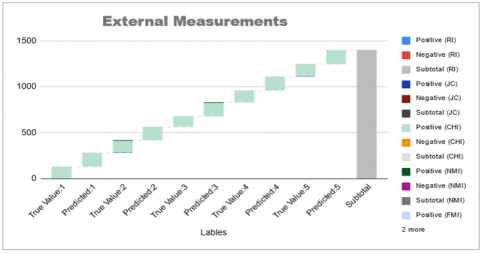
External Measurements (Rand Index-RI, Jaccard Coefficient-JC, Calinski-Harabasz Index-CHI, Normalized Mutual Information-NMI, and Fowlkes-Mallows Index-FMI) for predicted and true values, the predicted cluster assignments, and the true class labels or ground truth as indicated in Figure 5. The measurements for RI, JC, CHI, NMI, and FMI. The "Predicted Value" column represents the values obtained from the clustering algorithm, while the "True Value" column represents the values from the ground truth or true class labels.
Figure 5. Clustering measurements for external values
Table 6. External measurements for predicted and true value
|
Label’s |
RI |
JC |
CHI |
NMI |
FMI |
|
True Value:1 |
0.82 |
0.73 |
130.25 |
0.81 |
0.62 |
|
Predicted:1 |
0.75 |
0.65 |
150.21 |
0.88 |
0.75 |
|
True Value:2 |
0.78 |
0.71 |
128.32 |
0.75 |
0.61 |
|
Predicted:2 |
0.75 |
0.66 |
145.32 |
0.82 |
0.71 |
|
True Value:3 |
0.72 |
0.74 |
111.22 |
0.75 |
0.61 |
|
Predicted:3 |
0.75 |
0.66 |
145.32 |
0.83 |
0.71 |
|
True Value:4 |
0.82 |
0.73 |
130.25 |
0.81 |
0.62 |
|
Predicted:4 |
0.75 |
0.67 |
150.21 |
0.84 |
0.79 |
|
True Value:5 |
0.85 |
0.73 |
130.25 |
0.81 |
0.62 |
|
Predicted:5 |
0.79 |
0.65 |
150.21 |
0.88 |
0.75 |
Table 7. Internal measurements for predicted and true value in clustering
|
Label’s |
Silhouette Coefficient |
Dunn Index |
Davies-Bouldin Index |
|
True Value:1 |
0.73 |
0.75 |
0.68 |
|
Predicted:1 |
0.75 |
0.79 |
0.74 |
|
True Value:2 |
0.79 |
0.81 |
0.72 |
|
Predicted:2 |
0.81 |
0.83 |
0.78 |
|
True Value:3 |
0.75 |
0.92 |
0.79 |
|
Predicted:3 |
0.83 |
0.93 |
0.88 |
In the Rand Index, the true value is calculated as 0.82 after 1st iteration and the predicted value is 0.75, the true value is calculated as 0.78 after 2nd iteration, and the predicted value is 0.75, the true value is calculated as 0.72 after the 3rd iteration and the predicted value as 0.75, the true value is calculated as 0.82 after the 4th iteration and the predicted value as 0.75, the true value is calculated as 0.85 after 5th iteration and predicted values as 0.79.
In Jaccard Coefficient, the true value is calculated as 0.73 after 1st iteration, and the predicted value is 0.65, the true value is calculated as 0.71 after 2nd iteration and the predicted value is 0.66, the true value is calculated as 0.74 after 3rd iteration and predicted values as 0.66, the true value is calculating as 0.73 after 4th iteration and predicted values as 0.67, the true value is calculating as 0.73 after 5th iteration and predicted values as 0.65. Similarly, for JC, CHI, NMI, and FMI true value calculation is indicated in Table 6. Internal measurements such as the Silhouette Coefficient, Dunn Index, and Davies-Bouldin Index involve the comparison between predicted and true values as indicated in Table 7. Instead, they assess the quality of the clustering results based on the internal characteristics of the data and the clustering solution itself. Therefore, these measurements are typically presented in a table format comparing predicted and true values based on Volatile compounds and Principal Components Analysis.
4.7 Performance evaluation
Through the internal and external values calculation predicted and true values are observed using Volatile compounds and Principal Components Analysis. Performance is evaluated based on cluster models. Accuracy, Precision, Recall, and F1 score are calculated as shown in Eqs. (16)-(19).
Accuracy is the proportion of data points that have been appropriately grouped. It is computed as follows:
Accuracy =\frac{\text { number of correctly data points }}{\text { total number of data points }} (16)
Precision is defined as the percentage of data points labeled as belonging to a specific cluster that belongs to that cluster. It is determined as follows:
Precision= (number of correctly classified data points)/(total number of data points classified as belongs to that cluster) (17)
Recall is the percentage of data points labeled as belonging to a specific cluster that belong to that cluster. It is determined as follows:
Recall= (number of correctly classified datapoints)/(total number of data points that actually belongs to that cluster) (18)
The F1 score is the harmonic mean of precision and recall. It is determined as follows:
F 1 score =2 * \frac{\text { Precision } * \text { recall }}{\text { Precision }+ \text { Recall }} (19)
Classified as groups and subgroups of coffee aroma patterns that were already known. These groups could be classified on the kind of coffee, roasted level, and smell, and whether or not there are any diseases. These analyzed coffee flavor profiles into groups by using a method called hierarchical agglomerative clustering (HAC). They matched up the results of clustering with the known groups and subsets. The Jaccard index between the two sets of names was used to figure out how to do this. The Jaccard index is a way to figure out how much two sets are alike as shown in Eq. (14). Section 5 discusses the Results Analysis based on Principal Components Analysis for coffee aromas.
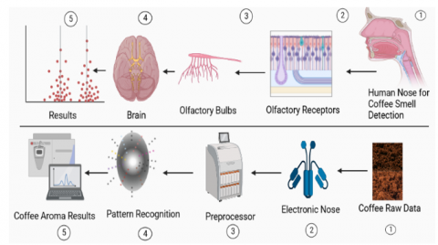
An electronic nose application is used to detect the coffee aroma based on the purity and quality of each stage based on Hierarchical Agglomerative Clustering for Identification, Quantification, and Disease Detection. In the existing work, coffee aroma is observed based on two qualities good or bad, stages of coffee aroma are not observed properly, and results are not accurate. In the current work, using electronic nose application by conducting polymer sensors. Coffee aroma is measured using internal and external measurements. Internal measurements are assessments or evaluations made by individuals based on their personal experience with the coffee fragrance. This encompasses fragrance notes, intensity, complexity, and overall quality. Internal measurements are subjective and based on own sensory perception. External measurements of coffee fragrance might refer to objective measurements or quantifiable factors. These measurements could include the use of analytical devices or techniques to evaluate certain characteristics of the fragrance. Gas chromatography-mass spectrometry (GC-MS), for example, can be used to identify and quantify distinct volatile components in coffee scents as indicated in Figure 6. Using the Hierarchical Agglomerative Algorithm, compare internal and exterior measures using predicted and true results. Internal Dimensions: Silhouette Coefficient: This metric assesses cluster tightness and separation. It can be determined given the HAA's expected cluster assignments.
Figure 6. Clustering measurements for internal values
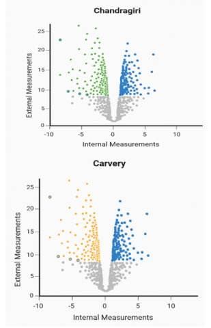
External Dimensions: Rand Index (RI): The RI compares the expected clustering result to the true class labels or ground truth. The Jaccard Coefficient (JC) quantifies the agreement between anticipated cluster assignments and genuine class labels. The Fowlkes-Mallows Index (FMI) assesses the similarity between predicted clustering and genuine class labels as indicated in Figure 7. Evaluation of currently available coffee smell predicts with multiple algorithms for Machine Learning Techniques that include support vector machine, Random forest, Convolution neural network, Gaussian Mixture Models, Artificial Neural Networks based on performance evaluation, and various volatile compounds released during the roasting process, as shown in Figure 8. Reviewed existing model Artificial Neural Network achieved 93.99%. After 15 iterations, the support vector machine (SVM) achieved a 74.8% accuracy, the Random forest algorithm achieved an 84.11% accuracy, the Convolution Neural Network achieved an 87.3% accuracy, and the Gaussian Mixture Models achieved a 91.78% accuracy.
Electronic nose applications that use conducting polymer sensors might be difficult to implement since they require a data acquisition system, pattern recognition, and a sensor array. Sensor readings are converted to digital signals, and individual coffee aromas are then identified. This is mostly used to assess the concentration of volatile organic compounds (VOCs) in the air. The e-nose can be used to check coffee quality, identify coffee varieties, and even diagnose coffee-related illnesses. The accuracy of VOC concentration measurements is impacted by environmental factors such as temperature, humidity, and pressure. If the measurements don't match up, the patterns might shift. Capturing up the aroma was a laborious process.
Figure 7. Comparing measurements for external and internal value with a coffee variety
Figure 8. Comparison between existing models
The primary objective of this study is to classify the aroma of coffee by considering both the roasting technique and the specific variety of coffee beans. In previous studies conducted before the roasting step, coffee berry stages were categorized to track the subsequent development of coffee aroma and identify any potential diseases. This study highlights the challenges of detecting many coffee aromas utilizing a Hierarchical Agglomerative Algorithm-created E-nose prototype. Principal Components Analysis compares organic volatile chemical aroma samples from different coffee aromas. Inspired by Machine Learning, external and internal parameters categorize coffee aroma. E-Nose's qualitative as well as quantitative performance and dependability have improved significantly after applying Machine Learning Techniques. The performance of testing samples was compared by accuracy. (1) Rand Index (RI), Jaccard Coefficient, Calinski-Harabasz Index, NMI, and Fowlkes-Mallows Index create external measures. (2) The Silhouette Coefficient, Dunn Index, and Davies-Bouldin Index are used to calculate internal measures and compare external and internal accuracy. Performance is evaluated based on cluster models. Accuracy, Precision, Recall, and F1 score achieved 97.08% accuracy in finding accurate coffee aroma. The future strategy will focus on coffee flavor with quality measurement in various stages of coffee progression using AI agents. This rigorous look at coffee aroma analysis and factory control can help manufacturers standardize operations, save money, and defend consumer rights.
Available based on Request.
[1] Jiang, Z., Lou, Y., Liu, X., Sun, W., Wang, H., Liang, J., Guo, J., Li, N., Yang, Q. (2023). Combined application of coffee husk compost and inorganic fertilizer to improve the soil ecological environment and photosynthetic characteristics of arabica coffee. Agronomy, 13(5): 1212. https://doi.org/10.3390/agronomy13051212
[2] Tavares, S., Azinheira, H., Valverde, J., Pajares, A.J.M., Talhinhas, P., Silva, M.D.C. (2023). Identification of HIR, EDS1, and PAD4 genes reveals differences between coffee species that may impact disease resistance. Agronomy, 13(4): 992. https://doi.org/10.3390/agronomy13040992
[3] Duana-Ávila, D., Hernández-Gracía, T.J., Martínez-Muñoz, E., García-Velázquez, M.D.R., Román-Gutiérrez, A.D. (2023). Study of the Mexican cocoa market: An analysis of its competitiveness (2010-2021). Agronomy, 13(2): 378. https://doi.org/10.3390/agronomy13020378
[4] Alharbi, M., Rajagopal, S.K., Rajendran, S., Alshahrani, M. (2023). Plant disease classification based on ConvLSTM U-Net with fully connected convolutional layers. Traitement du Signal, 40(1): 157. https://doi.org/10.18280/ts.400114
[5] Tamilvizhi, T., Surendran, R., Anbazhagan, K., Rajkumar, K. (2022). Quantum-behaved particle swarm optimization-based deep transfer learning model for sugarcane leaf disease detection and classification. Mathematical Problems in Engineering, 2022. https://doi.org/10.1155/2022/3452413
[6] Subahi, A.F., Khalaf, O.I., Alotaibi, Y., Natarajan, R., Mahadev, N., Ramesh, T. (2022). Modified self-adaptive Bayesian algorithm for smart heart disease prediction in IoT system. Sustainability, 14(21): 14208. https://doi.org/10.3390/su142114208
[7] Rajagopal, S., Thanarajan, T., Alotaibi, Y., Alghamdi, S. (2023). Brain tumor: Hybrid feature extraction based on UNet and 3DCNN. Computer Systems Science & Engineering, 45(2). http://dx.doi.org/10.32604/csse.2023.032488
[8] Zhang, L., Deng, P. (2017). Abnormal odor detection in the electronic nose via self-expression inspired extreme learning machine. IEEE Transactions on Systems, Man, and Cybernetics: Systems, 49(10): 1922-1932. https://doi.org/10.1109/TSMC.2017.2691909
[9] Fang, C., Li, H.Y., Li, L., Su, H.Y., Tang, J., Bai, X., Liu, H. (2022). Smart electronic nose enabled by an all-feature olfactory algorithm. Advanced Intelligent Systems, 4(7): 2200074. https://doi.org/10.1002/aisy.202200074
[10] Liu, H., Li, Q., Yan, B., Zhang, L., Gu, Y. (2018). Bionic electronic nose based on MOS sensors array and machine learning algorithms used for wine properties detection. Sensors, 19(1): 45. https://doi.org/10.3390/s19010045
[11] Tan, J., Xu, J. (2020). Applications of electronic nose (e-nose) and electronic tongue (e-tongue) in food quality-related properties determination: A review. Artificial Intelligence in Agriculture, 4: 104-115. https://doi.org/10.1016/j.aiia.2020.06.003
[12] Mu, F., Gu, Y., Zhang, J., Zhang, L. (2020). Milk source identification and milk quality estimation using an electronic nose and machine learning techniques. Sensors, 20(15): 4238. https://doi.org/10.3390/s20154238
[13] Xu, B., Moradi, M., Kuplicki, R., Stewart, J.L., McKinney, B., Sen, S., Paulus, M.P. (2020). Machine learning analysis of electronic nose in a transdiagnostic community sample with a streamlined data collection approach: No links between volatile organic compounds and psychiatric symptoms. Frontiers in Psychiatry, 11: 503248. https://doi.org/10.3389/fpsyt.2020.503248
[14] Hayasaka, T., Lin, A., Copa, V.C., Lopez Jr, L.P., Loberternos, R.A., Ballesteros, L.I.M., Kubota, Y., Liu, Y., Salvador, A.A., Lin, L. (2020). An electronic nose using a single graphene FET and machine learning for water, methanol, and ethanol. Microsystems & Nanoengineering, 6(1): 50. https://doi.org/10.1038/s41378-020-0161-3
[15] Dadi, P.S., Tamilvizhi, T., Surendran, R. (2022). Layout optimization for agriculture or small-scale agrarian industry. In 2022 6th International Conference on Trends in Electronics and Informatics (ICOEI). IEEE, pp. 174-179. https://doi.org/10.1109/ICOEI53556.2022.9777169
[16] Ye, Z., Liu, Y., Li, Q. (2021). Recent progress in smart electronic nose technologies enabled with machine learning methods. Sensors, 21(22): 7620. https://doi.org/10.3390/s21227620
[17] Suarez-Peña, J.A., Lobaton-García, H.F., Rodríguez-Molano, J.I., Rodriguez-Vazquez, W.C. (2020). Machine learning for cup coffee quality prediction from green and roasted coffee beans features. In Workshop on Engineering Applications. Cham: Springer International Publishing, pp. 48-59. https://doi.org/10.1007/978-3-030-61834-6_5
[18] Harsono, W., Sarno, R., Sabilla, S.I. (2020). Recognition of original arabica civet coffee based on odor using electronic nose and machine learning. In 2020 International Seminar on Application for Technology of Information and Communication (iSemantic), IEEE, pp. 333-339. https://doi.org/10.1109/iSemantic50169.2020.9234234
[19] Caporaso, N., Whitworth, M.B., Fisk, I.D. (2022). Prediction of coffee aroma from single roasted coffee beans by hyperspectral imaging. Food Chemistry, 371: 131159. https://doi.org/10.1016/j.foodchem.2021.131159
[20] Hendrawan, Y., Widyaningtyas, S., Fauzy, M.R., Sucipto, S., Damayanti, R., Al Riza, D.F., Hermanto, M.B., Sandra, S. (2022). Deep learning to detect and classify the purity level of luwak coffee green beans. Pertanika Journal of Science & Technology, 30(1): 1-18.
[21] García, M., Candelo-Becerra, J.E., Hoyos, F.E. (2019). Quality and defect inspection of green coffee beans using a computer vision system. Applied Sciences, 9(19): 4195. https://doi.org/10.3390/app9194195
[22] Angeloni, S., Mustafa, A.M., Abouelenein, D., Alessandroni, L., Acquaticci, L., Nzekoue, F.K., Petrelli, R., Sagratini, G., Vittori, S., Torregiani, E., Caprioli, G. (2021). Characterization of the aroma profile and main key odorants of espresso coffee. Molecules, 26(13): 3856. https://doi.org/10.3390/molecules26133856
[23] Thanarajan, T., Alotaibi, Y., Rajendran, S., Nagappan, K. (2023). Improved wolf swarm optimization with deep-learning-based movement analysis and self-regulated human activity recognition. AIMS Mathematics, 8(5): 12520-12539. https://doi.org/10.3934/math.2023629
[24] Raveena, S., Surendran, R. (2023). ResNet50-based classification of coffee cherry maturity using deep-CNN. In 2023 5th International Conference on Smart Systems and Inventive Technology (ICSSIT), IEEE, pp. 1275-1281. https://doi.org/10.1109/ICSSIT55814.2023.10061006
[25] Lee, C.H., Chen, I.T., Yang, H.C., Chen, Y.J. (2022). An AI-powered electronic nose system with fingerprint extraction for aroma recognition of coffee beans. Micromachines, 13(8): 1313. https://doi.org/10.3390/mi13081313
[26] Dewangan, S., Rao, R.S., Mishra, A., Gupta, M. (2022). Code smell detection using ensemble machine learning algorithms. Applied Sciences, 12(20): 10321. https://doi.org/10.3390/app122010321
[27] Zhang, W., Liu, T., Ye, L., Ueland, M., Forbes, S.L., Su, S.W. (2019). A novel data pre-processing method for odor detection and identification system. Sensors and Actuators A: Physical, 287: 113-120. https://doi.org/10.1016/j.sna.2018.12.028
[28] Gonzalez Viejo, C., Tongson, E., Fuentes, S. (2021). Integrating a low-cost electronic nose and machine learning modeling to assess coffee aroma profile and intensity. Sensors, 21(6): 2016. https://doi.org/10.3390/s21062016
[29] Tanveer, M., Khan, H.H., Malik, M.N., Alotaibi, Y. (2023). Green requirement engineering: Towards sustainable mobile application development and internet of things. Sustainability, 15(9): 7569. https://doi.org/10.3390/su15097569
[30] Raveena, S., Surendran, R. (2023). Clustering-based hemiplegia vastatrix disease prediction in coffee leaf using deep belief network. In 2023 8th International Conference on Communication and Electronics Systems (ICCES), IEEE, pp. 1094-1100. https://doi.org/10.1109/ICCES57224.2023.10192835
[31] KAGGLE Dataset. Coffee Quality Database from CQI. https://www.kaggle.com/datasets/volpatto/coffee-quality-database-from-cqi, accessed on Aug. 12, 2022.
[32] qacData. Coffee Quality Institute Database. https://rkabacoff.github.io/qacData/reference/coffee.html, accessed on Nov. 10, 2020.