Aditya G. Manjunath | Sabahudin Vrtagić* | Fatih Dogan | Milan Dordevic | Mileta Zarkovic | Jasmin Kevric | Goran Dobric
© 2021 IIETA. This article is published by IIETA and is licensed under the CC BY 4.0 license (http://creativecommons.org/licenses/by/4.0/).
OPEN ACCESS
This research paper deals with the problem of Metal-Oxide Surge Arrester (MOSA) condition monitoring and a new methodology in surge arrester monitoring and diagnostics is presented. A machine learning algorithm (back propagation regression) is used to estimate the non-linearity coefficient of the surge arrester, based on operating voltage and leakage current of the arrester. Using a simulated system, this research investigates the possibility of application and efficiency of machine learning. It is shown that the applied learning algorithm results are competitive with the model results parameters calculated as R2 = 0.999 and mean absolute real error computed as 0.005 which has shown that the proposed model can be used for MOSA monitoring and diagnostic purposes.
metal-oxide surge arrester (MOSA), Fourier transform, machine learning, regression, simulated system
Metal-oxide surge arresters (MOSAs) play an important role in power system protection. Malfunction of MOSAs can cause dangerous overvoltage which can damage electrical power equipment and endanger human life. Therefore, periodical monitoring of MOSAs has to be conducted in order to diagnose their condition. There are many contributions related to monitoring indicators and diagnostic procedures. Some of them are based on on-line monitoring while the others investigate off-line monitoring procedures. Newly developed MOSA monitoring methods are based on artificial intelligence [1-6]. Most researches propose the measurement of leakage current in order to extract MOSA’s condition indicators [7-14]. These indicators are mostly 1st or 3rd order harmonic of resistive current component, and 3rd order harmonic of total current. The reason for current leakage distortion results in the mentioned harmonic components. Therefore, even with pure sine wave operating voltage, the current leakage is distorted. It has been shown that the level of non-linearity, consequently the level of leakage current distortion, depends on the condition of MOSA. The more degraded the arrester is, the higher the current and all of the mentioned indicators are. This happens due to reduced non-linearity of the arrester with degradation.
Nevertheless, leakage current is not only dependent on MOSA condition but also on operating voltage, voltage harmonics and ambient conditions. This is why the reliability of the current based indicators has been questioned. Instead, non-linearity coefficient of MOSA is a physical parameter that does not depend on voltage harmonics, operating voltage level or ambient conditions, except temperature. This statement has been fully elaborated in [15]. Namely, non-linearity coefficient should be observed as resistance. The resistance of an element does not change at different applied voltages. The resistance only changes due to temperature change if it is heated by current flowing through the resistor or an external heat source. This implies that non-linearity coefficient, if estimated, represents one of the best indicators of MOSA. The previous conclusion is based on the fact that condition indicators should only be sensitive to condition of an element, clearly showing whether the element is new or degraded. If an indicator is sensitive to other parameters, let's say voltage harmonics, it can falsely indicate that a new element is old if it is operated in the condition with high voltage harmonics. More details and analysis about reliability of MOSA indicators are given in [15].
Currently, methods that estimate non-linearity coefficient of MOSA are based on the assumption that MOSA equivalent circuit is known. Moreover, these methods use simplified MOSA circuits that have some discrepancies when compared to real surge arrester. This causes errors in the obtained results of non-linearity coefficient. The authors propose the elimination of equivalent circuit from the estimation methodology by using machine learning system that can be trained on real measurement data. Therefore, instead of using simplified MOSA model, MOSA machine learning system is used to represent MOSA behavior.
The proposed machine learning system estimates non-linearity coefficient of MOSA using operating voltage and leakage current as input values. As voltage and current are measured as time domain signals, Fourier transform is used to make them appropriate input parameters. The simulation is performed to prepare training, validation and test data for the system.
A different approach of using machine learning algorithm in the enhancing voltage stability of multi-machine power system have been shown in [16] which was used for alteration of the parameters of the static var compensator controller. The authors in [17] used the back propagation neural network algorithm for time sequence prediction. They showed that the caution threshold can be used to alarm about abnormalities and estimate the abnormal probability. Fuzzy expert system is also applied in MOSA monitoring procedure [18].
As a learning algorithm, back-propagation is used to train the neural network. The upsides of the back propagation neural network strategy over conventional classifiers are its nonparametric nature, simple variation to innumerable varieties of data and information structures.
The paper is systematized as follows: Introduction and background deliver an insight of the problem. Methodology section explains the MOSA simulation and presents machine learning system. The full procedure details used in this study to obtain non-linearity coefficient is given also in methodology section. The upshots of research strays using the presented research mock-ups and their discussion are presented in the result section. Finally, the last section delivers concluding contemplations with specific standards and instructions for further research.
The neural network architectures depend on back-spread to diminish or reduce the miscalculations. The planning design of data is done by framing portrayal in the hidden layers. This ability of back-propagation, as it is shown in [15], is suitable for the problems where no direct known relationship is found. The adaptability and learning abilities of back propagation has been effectively carried out in wide scope of uses.
Moreover, the important updates are given by learning rate and momentum used to speed-up the system convergence. Back-propagation with Fixed Momentum (BPFM) is typical methods that is applied to haste up convergence and preserve optimal performance. The short come of the BPFM is that update of the weights is in the upward direction instead of downward. Therefore, the momentum should be varied rather than keeping it fixed as shown in [16, 17]. The energy coefficient updates consider all the weights in the Multi-layer Perceptron (MLP) to assure its main advantage. The neural net with the Gradient Descent Back Propagation Algorithm (GDAM) has been used for all grouping issues unlike the past methods [19-21]. Back-spread calculations using the force, speed and angle updates are shown to have an impact on the learning rate. Utilizing the optimum initialization technique guarantees that the yield neurons are in the dynamic district and that the scope of enactment work is completely used [22-24]. The ideal introduction technique has been executed on worthless equality issues, four-bit equality checkers, and encoder issues as demonstrated in ref. [25, 26].
The additional important updates are a technique that uses Variation Auto-Encoder (VAE) demonstrated in ref. [27, 28]. The given network is inferential network that tries to regularize the back dispersion of the inactive elements. It has been shown that VAE doesn't perform the express clarify away induction. The other commonly used strategy is the Generative Adversarial Networks (GAN) [29, 30]. The helping network is a discriminator network that assumes an ill-disposed part against the generator organization. The GAN tries not to deduce the dormant factors. Experiments conducted [31] showed that the rotating back-spread calculation is more straightforward and more fundamental, without turning to an additional organization. It outlines the strength of rotating back-propagation by gaining from inadequate and backhanded information. In the interim, substituting back-spread is correlative to VAE and GAN preparing. It might utilize VAE to introduce the inferential back-engendering, and subsequently, may improve the induction in VAE. Furthermore, it may help derive the inert variables of the noticed models for GAN, subsequently giving a technique to test if it can clarify the whole preparing set as shown in [31, 32].
3.1 MOSA simulation
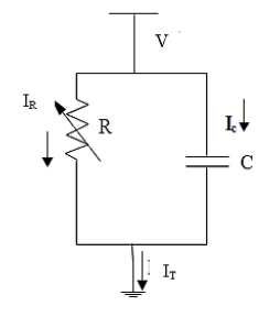
In order to design the machine learning system, computer simulations of MOSA are conducted. In these simulations, the widely accepted simplified arrester equivalent circuit is used (Figure 1).
Figure 1. MOSA equivalent circuit
In Figure 1, total leakage current (IT) comprises of two components: capacitive current (Ic) and resistive current (IR). Capacitance of the arrester is linear while the resistance is non-linear. The leakage current can be calculated according to:
$I_{T}=C \cdot \frac{d V}{d t}+I_{r e f} \cdot K \cdot\left(\frac{V}{V_{r e f}}\right)^{\alpha}$, (1)
where, C is capacitance, V is the operating voltage, Iref and Vref are reference values of current and voltage, while K is constant. Capacitance, as proven before, doesn’t change due to MOSA condition. Therefore, it has been kept constant in the simulations. The only parameter that changes due to degradation is the non-linearity coefficient α. This parameter has been varied in the simulations between the values of 2 and 7 randomly. Additionally, operating voltage usually contains harmonics. These harmonics also affect the leakage current. Therefore, the simulations include randomly changing voltage harmonics up to the 11th order. All harmonics change the value of the voltage in the range of 0 to 5%. In addition, each harmonic phase can take any value between 0° and 90°.
Combining all components, the simulation algorithm is as follows:
1. Enter capacitance value
2. Randomly select the non-linear coefficient in the range 2 to 7.
3. Randomly select operating voltage harmonics (3rd, 5th, 7th, 9th and 11th) in the range 0 to 5%.
4. Randomly select the 1st order of voltage in the range 90 to 110% of rated value.
5. Calculate leakage current according to Eq. (1).
6. Use Fourier transform on leakage current to obtain first 25 harmonics.
After initializing the simulation, leakage current and operating voltage harmonics are used as input parameters to the machine learning system. Non-linearity coefficient is used as the output value. After training, the system is able to estimate the non-linearity coefficient for any input values of voltage and current. This system can be used for real MOSA with measured values of voltage and current as its inputs to estimate the real value of non-linearity coefficient.
3.2 Machine learning system
The Broyden-Fletcher-Goldfarh-Shanno (BFGS) algorithm decides the plunge heading by preconditioning the angle with arch data. It performs by progressively improving estimation to the Hessian matrix of the misfortune work, gotten uniquely from gradient evaluations [33-35].
BFGS enhancement calculation is typically utilized for nonlinear calculations. By introducing least squares, multilayer perceptron (MLP) achieves faster training and better accuracy. The methodology line introduced in the paper comprise of three main stages:
(1) Data set normalization with standard scalar and robust scalar;
(2) Introducing “logistic” span of the activation function;
(3) Calculating the gradient descent of individual errors with respect to the weights and gains values. The MLP learns iteratively the halfway subordinates of the misfortune works on the improvements of the model accuracy.
The new methodology improved the preparation proficiency of back engendering calculation by adaptively changing the underlying inquiry bearing, demonstrated by BFGS given by scikit-learn libraries [36].
Feature scaling of a dataset is a typical prerequisite for AI assessors. Normally, this is completed by eliminating the mean and scaling to unit variance. Notwithstanding, anomalies can frequently impact the mean/fluctuation in a negative manner. In such cases, the median and the local range regularly give better outcomes [37]. As mentioned, the first step is to scale input parameters or to find the best fit for controlling the size of a vector in an iterative cycle, a boundary vector during preparation for example, to evade mathematical hazards because of quantity variation. One of the key points to create a successful model is to optimize input parameter variation, the mentioned harmonics, voltages (V) and currents (I) inputs. RobustScaler and StandardScaler preprocessing functions within scikit-learn libraries are used so that an understanding and effects of the fluctuation can be observed. The functions mentioned above eliminate the variance in the dataset per the quintile range by focusing and scaling individually on each feature by computing the relevant statistics on the samples in the training set input parameters.
The goal of MLP regressor training can be expressed as optimization of a cost function and can be formulated as
$E_{\text {True }}=\int_{E, y} e(f(x, w), d) p(x, y) d x d y$, (2)
where, “e” denotes a local cost function, “f” is the BFGS function implemented by the MLP, “x” are model inputs (19981 points for each set), “y” is the anticipated output, “w” denotes the weights in the system, and p symbolizes the probability dispersal. The impartial of training is to adjust the parameters “w” such that ETrue is diminished where ETrue, denotes the generalization error. Methods used to prevent overfitting in MLP are: model choice, early ending, weight deterioration, and pruning [38-40].
In order to confirm model results or predictions, different error parameters are calculated with the main focus on the mean absolute error (MAE), root mean squared error (RMSE) and R-squared.
$M E A=\frac{1}{m} \sum_{k=1}^{m}\left|y_{k}-¥_{k}\right|$, (3)
where, $¥_{k}$ represents predicted values for interval k and yk represents the real output. Similarly, the RMSE formula is given as:
$R M S E=\sqrt{\frac{1}{m} \sum_{k=1}^{m}\left(y_{k}-¥_{k}\right)^{2}}$. (4)
Both MAE and RMSE characterize normal model expectation mistake with the units of the variable of interest where the two measurements can go from 0 to ∞ and are apathetic regarding the course of blunders. They are called contrarily arranged scores which mean that lower esteems address a superior model.
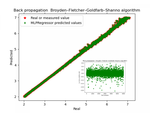
The final dataset used for training is created from the 32 harmonics with total of 20000 sample inputs where 70% is used for training and 30% for testing. The results in Figures 2 and 3 and Tables 1-3 show very good accuracy for the model.
Figure 2. StandardScaler MLP predictions on test data. Green color diamonds represent the real alpha reading (no unit) and the red stars represent predicted value
All the MLP prediction is performed using random datasets, with the same training to testing ratio. The MLP model trains using the back-propagation algorithm based on the least square error as the loss function which optimizes the squared-loss using limited-memory-BFGS. The MLP model errors and accuracy parameters are given in Table 1.
In Table 1, the error outputs are shown for both methodologies within the MLP model. The difference in accuracy is negligible. This indicates there aren’t many outlying points in the dataset used within our testing inputs. Overall, the error parameters indicate that the MLP model precision is very high with $R^{2}=0.999$ and mean absolute real error computed as 0.005 for both scalers. This has shown that the proposed model can be used for MOSA monitoring and diagnostic purposes.
Figure 3. RobustScaler MLP predictions on test data
Table 1. MLP parameters and errors
|
Scaling techniques |
Standard Scaler |
Robust Scaler |
|
Absolute relative error of the mean |
0.005 |
0.005 |
|
median_abs_error |
0.013 |
0.014 |
|
rmse |
0.032 |
0.036 |
|
rmsle |
0.005 |
0.006 |
|
rmspe |
0.006 |
0.007 |
|
rmsse |
0.021 |
0.024 |
|
rrse |
0.024 |
0.027 |
|
r2_mod |
0.999 |
0.999 |
|
nse_bound |
0.999 |
0.999 |
|
nse_mod |
0.982 |
0.981 |
|
nse_rel |
1 |
0.999 |
To be more vibrant, a tabular form of the data with new output parameters and the MLP predictions are shown in Table 2 with corresponding error. The “Real”$\alpha$ parameter is MATLAB simulation result of the dataset whereas the “Predicted” values are the output of MLP model presented here.% Error is the percent discrepancy between the Real and Predicted values.
Table 2. MLP results on new a new input data
|
MATLAB |
Standard Scaler |
Robust Scaler |
||
|
Real |
Predicted |
% Error |
Predicted |
% Error |
|
5.736 |
5.72055 |
0.269391 |
5.70604 |
0.522392 |
|
5.2938 |
5.29456 |
0.0143454 |
5.3097 |
0.300301 |
|
4.5853 |
4.56463 |
0.450874 |
4.56253 |
0.496687 |
|
2.8952 |
2.89138 |
0.131932 |
2.90747 |
0.423732 |
|
3.0171 |
3.02252 |
0.179704 |
3.01138 |
0.189468 |
|
4.1989 |
4.17175 |
0.64651 |
4.18125 |
0.420329 |
|
2.5196 |
2.52097 |
0.0542386 |
2.52792 |
0.330396 |
|
4.6163 |
4.62211 |
0.125937 |
4.56811 |
1.04381 |
|
3.7707 |
3.76115 |
0.253349 |
3.74029 |
0.806423 |
|
5.6426 |
5.61984 |
0.403319 |
5.62949 |
0.232389 |
|
4.053 |
4.07315 |
0.497093 |
4.0669 |
0.343048 |
|
3.957 |
3.95151 |
0.138698 |
3.95581 |
0.02996 |
|
5.8245 |
5.84609 |
0.370758 |
5.83534 |
0.186136 |
The results given in Table 2 have shown the model prediction on the unknown input, which is the key point that describe the model accuracy. In combination with Table 1, the overall model results are very precise. Error parameters presented in Table 1 are based on the testing stage with 5995 inputs, which is 30% of the total amount of the data. For all outputs, the error values (Table 1) are very small while the output values (Table 2) are very close to the expected value obtained from MATLAB.
Besides the non-linearity coefficient, other indicators are also used for MOSA monitoring and diagnostics. These indicators are: the first order of resistive current component (Ir1), the third order of resistive current component (Ir3), the maximum value of resistive current (Irm), active power losses (P). Different methods are used to estimate these parameters. These methods are: harmonic analysis (HARM), direct method (DIR), active power method (P), iterative method (ITER), and point on wave method (POW), variable coefficient compensation method (VCC), compensation method (COM), and genetic algorithm method (GA).
So far, only GA method estimates the value of non-linearity coefficient [4]. This method has been analyzed in three different cases: (1) changing the nonlinearity coefficient; (2) changing fundamental voltage harmonic between 0.9 and 1.1 of rated value and (3) adding higher order voltage harmonics. The estimation errors in all of these cases have proven that GA performs extremely well. The GA outcomes are displayed in Table 3. Table 3 can be used to relate the results with the newly suggested method which has shown that MLP can achieve better accuracy than GA and that it represents a potential method for future MOSA monitoring and diagnostics algorithms. MLP has been tested for all three cases at the same time, so the error is presented as a unique range for all three cases, taken from Table 2.
Table 3. Indicator estimation relative errors
|
Methods |
Errors |
Changing non-linearity coefficient |
Changing voltage RMS |
Changing voltage harmonics |
|
GA |
δα [%] |
0.56 |
0.42 |
0.75 |
|
MLP |
δα [%] |
0.014 – 1.044(average from Table 2 0.40) |
||
Taking into consideration that GA is based on MOSA equivalent circuit equations it can be concluded that GA algorithm is more prone to errors due to simplifications behind the equivalent circuit.
The paper shows that machine learning can be used for MOSA monitoring and diagnostics. The created MLP model is used to estimate MOSA non-linearity coefficient based on leakage current and voltage input parameters. The input-output parameters are generated by MATLAB script where harmonics of the operational voltage and leakage current are used as input and non-linearity coefficient α as the output parameter. After input scaling, a MLP back propagation model is used to train, so that the corresponding weights can be obtained. The prediction results are evaluated by calculating different error values which demonstrated that the MLP can be used as a trustworthy tool for non-linearity prediction. Considering that non-linearity is a great indicator of MOSA condition, the proposed methodology can be used for MOSA diagnostics. Additional testing is performed by preserving some of the input output data which was used for error calculations. The obtained results meet satisfaction with all calculated errors less than 1%. Additionally, comparing the achieved results to other methods, like GA, showed that the proposed machine learning method is effective and provides better results in various scenarios. Therefore, the suggested machine learning algorithm is competitive in estimation of non-linear coefficient, particularly taking into consideration that the algorithm improves itself over time.
[1] Guo, H., Tang X.F., Chang, Z.W., Fang, Y. (2014). Application kohonen neural network to MOA fault diagnosis. Applied Mechanics and Materials, 568-570: 874-878. https://doi.org/10.4028/www.scientific.net/AMM.568-570.874
[2] Novizon, Y., Zulkurnain, A.M. (2014). Correlation between third harmonic leakage current and thermography image of zinc oxide surge arresters for fault monitoring using artificial neural network. Applied Mechanics and Materials, 554: 598-602. https://doi.org/10.4028/www.scientific.net/AMM.554.598
[3] Lira, G.R.S., Costa, E.G., Ferreira, T.V. (2014). Metal-oxide surge arrester monitoring and diagnosis by self-organizing maps. Electric Power Systems Research, 108: 315-321. http://doi.org/10.1016/j.epsr.2013.11.026
[4] Dobric, G., Stojanovic, Z., Stojkovic, Z. (2015). The application of genetic algorithm in diagnostics of metal-oxide surge arrester. Electric Power Systems Research, 119: 76-82. http://doi.org/10.1016/j.epsr.2014.09.009
[5] Khodsuz, M., Mirzaie, M. (2015). Monitoring and identification of metal–oxide surge arrester conditions using multi-layer support vector machine. IET Gener. Transm. Distrib., 9(16): 2501-2508. http://doi.org/10.1049/iet-gtd.2015.0640
[6] Dobric, G., Stojanovic, Z., Stojkovic, Z. (2015). MOSA monitoring using unsynchronised measurements of voltage and leakage current. Mediterranean Conference on Power Generation, Transmission, Distribution and Energy Conversion, MedPower2015, Belgrade, Serbia. http://doi.org/10.1049/cp.2016.1015
[7] Heinrich, C., Hinrichsen, V. (2001). Diagnostics and monitoring of metal-oxide surge arresters in high-voltage networks-comparison of existing and newly developed procedures. IEEE Transactions on Power Delivery, 16(1): 138-143. http://doi.org/10.1109/61.905619
[8] Xu, Z.N., Zhao, L.J., Ding, A., Lü, F.C. (2013). A current orthogonality method to extract resistive leakage current of MOSA. IEEE Transactions on Power Delivery, 28(1): 93-101. https://doi.org/10.1109/tpwrd.2012.2221145
[9] De Souza, R.T., Da Costa, E.G., Naidu, S.R., Maia, M.J.A. (2004). A virtual bridge to compute the resistive leakage current waveform in ZnO surge arresters. IEEUPES Transmission 8 Distribution Conference 8 Exposition: Latin America (IEEE Cat. No. 04EX956), Sao Paulo, Brazil. https://doi.org/10.1109/TDC.2004.1432387
[10] Zhu, H.X., Raghuveer, M.R. (2001). Influence of representation model and voltage harmonics on metal oxide surge arrester diagnostics. IEEE Transactions on Power Delivery, 16(4): 599-603. https://doi.org/10.1109/61.956743
[11] Wang, Y.Q., Lu, F.C. (2003). Influence of power system's harmonic voltage on leakage current of MOA. Asia-Pacific Conference on Environmental Electromagnetics, Hangzhou. China. https://doi.org/10.1109/CEEM.2003.238139
[12] Novizon, Abdul-Malek, Z., Bashir, N., Sayuti, A. (2011). Condition monitoring of zinc oxide surge arresters. Practical Applications and Solutions Using LabVIEWTM Software: InTech. https://doi.org/10.5772/23761
[13] Das, A.K., Dalai, S. (2021). Recent development in condition monitoring methodologies of MOSA employing leakage current signal: A review. IEEE Sensors Journal, 21(13): 14559-14568. https://doi.org/10.1109/JSEN.2021.3073536
[14] Barannik, M., Kolobov, V. (2020). System for monitoring the condition of metal-oxide surge arresters in service. In 2020 International Multi-Conference on Industrial Engineering and Modern Technologies (FarEastCon), Vladivostok, Russia, pp. 1-6. https://doi.org/10.1109/FarEastCon50210.2020.9271582
[15] Dobric, G., Stojkovic, Z., Stojanovic, Z. (2020). Experimental verification of monitoring techniques for metal-oxide surge arrester. IET Generation, Transmission & Distribution, 14(6): 1021-1030. https://doi.org/10.1049/iet-gtd.2019.1398
[16] Machavarapu, S., Rao, M.V.G., Rao, P.V.R. (2019). Machine learning algorithm based static VAR compensator to enhance voltage stability of multi-machine power system. Mathematical Modelling of Engineering Problems, 6(4): 641-649. https://doi.org/10.18280/mmep.060420
[17] Zhao, W., Li, Y.J., Ren, J.Y., Chen, S.G., Li, Y.Q. (2018). A novel operation state prediction method for servers in smart grids. European Journal of Electrical Engineering, 20(3): 379-392. https://doi.org/10.3166/EJEE.20.379-392
[18] Dobrić, G., Žarković, M. (2021). Fuzzy expert system for metal-oxide surge arrester condition monitoring. Electrical Engineering, 103(1): 91-101. https://doi.org/10.1007/s00202-020-01061-z
[19] Anil, K., Ankit, G., Gaurav, M., Rahul, R. (2005). A variant of back propagation algorithm for feed forward network. International Conference «Information Research & Applications».
[20] Denton, E.L., Chintala, S., Fergus, R. (2015). Deep generative image models using a laplacian pyramid of adversarial networks. Computer Vision and Pattern Recognition (cs.CV), arXiv:1506.05751.
[21] Goodfellow, I.J., Pouget-Abadie, J., Mirza, M., Xu, B., Warde-Farley, D., Ozair, S., Courville, A., Bengio, Y. (2014). Generative adversarial nets. NIPS, pp. 2672-2680.
[22] Gunaseeli, N., Karthikeyan, N. (2007). A constructive approach of modified standard backpropagation algorithm with optimum initialization for feedforward neural networks. International Conference on Computational Intelligence and Multimedia Applications (ICCIMA 2007), Tamil Nadu, India, pp. 325-331. https://doi.org/10.1109/ICCIMA.2007.259
[23] Kingma, D.P., Welling, M. (2014). Auto-encoding variational bayes. ICLR, pp. 30-37.
[24] Lawrence, S., Giles, C.L. (2000). Overfitting and neural networks: conjugate gradient and backpropagation. In Proceedings of the IEEE-INNS-ENNS International Joint Conference on Neural Networks. IJCNN 2000. Neural Computing: New Challenges and Perspectives for the New Millennium, 1: 114-119. http://dx.doi.org/10.1109/IJCNN.2000.857823
[25] Lu, Y., Zhu, S.C., Wu, Y. (2016). Learning FRAME models using CNN filters. In Proceedings of the AAAI Conference on Artificial Intelligence, 30(1). https://ojs.aaai.org/index.php/AAAI/article/view/10238
[26] Mitchell, R.J. (2008). On simple adaptive momentum. 2008 7th IEEE International Conference on Cybernetic Intelligent Systems, London, UK, pp. 1-6. https://doi.org/10.1109/UKRICIS.2008.4798940
[27] Naw, N.M., Ransing, M.R., Ransing, R.S. (2006). An improved learning algorithm based on the broyden-fletcher-Goldfarb-Shanno (BFGS) method for back propagation neural networks. Sixth International Conference on Intelligent Systems Design and Applications, Jian, China, pp. 152-157. https://doi.org/10.1109/ISDA.2006.95
[28] Pedregosa, F., Varoquaux, G., Gramfort, A., Michel, V., Thirion, B., Grisel, O., Blondel, M., Prettenhofer, P., Weiss, R., Dubourg, V., Vanderplas, J., Passos, A., Cournapeau, D., Brucher, M., Perrot, M., Duchesnay, É. (2011). Scikit-learn: Machine learning in python. JMLR, 12: 2825-2830. http://jmlr.org/papers/v12/pedregosa11a.html.
[29] Buitinck et al. (2013). API design for machine learning software: experiences from the scikit-learn project, 108-122. arXiv:1309.0238.
[30] Radford, A., Metz, L., Chintala, S. (2016). Unsupervised representation learning with deep convolutional generative adversarial networks. ICLR. arXiv:1511.06434.
[31] Rehman, M.Z., Nawi, N., Ghazali, M.I. (2011). Noise-induced hearing loss (NIHL) prediction in humans using a modified back propagation neural network. International Journal on Advanced Science Engineering and Information Technology, 1(2): 185-189. https://doi.org/10.18517/ijaseit.1.2.39
[32] Rehman, M.Z., Nawi, N.M. (2011). Improving the accuracy of gradient descent back propagation algorithm (GDAM) on classification problems. IJNCAA, pp. 838-847. http://citeseerx.ist.psu.edu/viewdoc/download?doi=10.1.1.831.3920&rep=rep1&type=pdf.
[33] Rumelhart, D.E., Hinton, G.E., Williams, R.J. (1986). Learning internal representations by back-propagation errors. Nature, 323: 533-536. https://doi.org/10.1038/323533a0
[34] Shao, H., Zheng, H. (2005). A new BP algorithm with adaptive momentum for FNNs training. GCIS 2009, Xiamen, China, pp. 16-20. https://doi.org/10.1109/GCIS.2009.136
[35] Sotiropoulos, D., Kostopoulos, A., Grapsa, T.N. (2002). A spectral version of Perry's Conjugate gradient method for neural network training. 4th GRACM Congress on Computational Mechanics, pp. 291-298.
[36] Swanston, D.J., Bishop, J.M., Mitchell, R.J. (1994). Simple adaptive momentum: New algorithm for training multilayer Perceptrons. J. Electronic Letters, 30(18): 1498-1500. https://doi.org/10.1049/el:19941014
[37] Weigend, A., Rumelhart, D., Huberman, B. (1991). Generalization by weight-elimination with application to forecasting. Advances in Neural Information Processing Systems, pp. 875-882.
[38] Weiss, S.M., Kulikowski, C.A. (1991). Computer systems that learn: classification and prediction methods from statistics, neural nets, machine learning, and expert systems. Morgan Kaufmann Publishers Inc. https://dl.acm.org/doi/abs/10.5555/102700
[39] Xie, J., Lu, Y., Zhu, S.C., Wu, Y.N. (2016). A theory of generative convnet. ICML. http://proceedings.mlr.press/v48/xiec16.pdf.
[40] Zweiri, Y., Seneviratne, L.D., Althoefer, K. (2005). Stability analysis of a three-term back-propagation algorithm. J. Neural Networks, 18(10): 1341-1347. https://doi.org/10.1016/j.neunet.2005.04.007