Baohai Yang
OPEN ACCESS
The traditional fractional lower-order (FLO) spectrum estimation method cannot observe a sufficient volume of data, leading to a large variance of estimation results. To solve the problem, this paper puts forward a FLO bi-spectrum estimation method based on autoregressive (AR) model, and gives new definitions for FLO three order cumulant. The author discussed the determination of AR model parameters, and introduced how to implement the bi-spectrum estimation method based on AR model. Then, a series of tests were performed to verify the correctness of our method. The results show that our method outperformed the traditional approaches in suppressing FLO noise and identifying relevant information of signals.
autoregressive (AR) model, bi-spectrum, fractional lower-order (FLO) statistics, three order cumulant, signal processing
In the field of signal processing, the noise is mostly described by Gaussian distribution model, which has an excellent effect on two-order statistics of normal distribution [1]. When it comes to the frequency-domain analysis of noise, the existing theoretical methods include spectral feature analysis, time-frequency analysis, spectrum estimation, colored noise whitening, spatial spectrum estimation, frequency estimation, harmonic estimation and spectral line restoration. Most of these methods are based on two-order statistics like bi-spectrum and tri-spectrum [2].
Gaussian white noise and colored noise models have always occupied the leading position in signal processing, and the criterion of white noise and colored noise based on correlation function and power spectral density has been regarded as a classical rule. In practical applications, however, many noises do not conform to the normal distribution. Typical examples include low-frequency atmospheric noise and underwater noise. A viable option to describe such noises lies in setting up an α stable distribution, whose statistical features can be characterized by the relevant parameters of the feature function [3].
The best way to solve the non-Gaussian α stable distribution is the fractional lower-order (FLO) statistics. If α is greater than 2, the harmonic frequencies can be estimated accurately; otherwise, the second-order matrix does not exist, making it impossible to effectively analyze the noise [2]. To solve the problem, the FLO bi-spectrum has been conceptualized. Traditionally, the lower-order bi-spectrum is estimated by bi-spectrum and nonparametric methods. Nonetheless, these methods cannot observe a sufficient volume of data, leading to a large variance of estimation results.
In view of the above, this paper puts forward an FLO bi-spectrum estimation method based on autoregressive (AR) model [5], and compares the method with traditional approaches. The comparison shows that our method outperformed the traditional ones in spectral flatness and suppression of FLO noise.
This section briefly introduces the α stable distribution, a generalized conceptual Gaussian distribution with a wide application scope, and gives the definition to the relevant FLO statistics, which is the best way to filter the noise of non-Gaussian α stable distribution.
A random variable X satisfies the α stable distribution if the parameters 0≤α≤2, γ≥0 and -1≤β≤1 have the following relationship with real numbers α:
$\varphi (t)=\exp \{jat-\gamma {{\left| t \right|}^{a}}[1+j\beta sgn (t)\omega (t,\alpha )]\}$ (1)
where
$\omega (t,\alpha )=\left\{ \begin{matrix}\begin{matrix} \tan (\pi \alpha /2), & \alpha \ne 1 \\\end{matrix} \\ \begin{matrix}(2/\pi )\log \left| t \right|, & \alpha =1 \\\end{matrix} \\\end{matrix} \right.$
$sgn (t)=\left\{ \begin{matrix}\begin{matrix} 1, & t>0 \\\end{matrix} \\\begin{matrix} 0, & t=0 \\\end{matrix} \\\begin{matrix} -1, & t<0 \\\end{matrix} \\\end{matrix} \right.$
Note that α is a feature index in the interval (0, 2]. The index determines the shape of the distribution. The value of the index is negatively correlated with the trailing thickness and the pulse feature [6].
(1) FLO moments. The FLO moments refer to the various moments existing at 0<α<2 (i.e. the absence of secondary moment). For the random variable SαS, the FLO moments can be described by its dispersion coefficient and feature index. Meanwhile, the covariation of the two random variables η and ζ can be expressed as the function of FLO moments:
${{\left[ \xi ,\eta \right]}_{\alpha }}=\frac{E\left( \xi {{\eta }^{<p-1>}} \right)}{E\left( {{\left| \eta \right|}^{p}} \right)}{{\gamma }_{\eta }}$ (2)
where the right superscript * is a complex conjugate; γη is the bias coefficient of the stochastic process η:
$\gamma _{\eta }^{p/\alpha }=\frac{E\left( {{\left| \eta \right|}^{p}} \right)}{C\left( p,\alpha \right)}\begin{matrix}, & 0<p<\alpha \\\end{matrix}$ (3)
where
$C\left( p,\alpha \right)=\frac{{{2}^{p+1}}\Gamma \left( \frac{p+2}{2} \right)\Gamma \left( -\frac{p}{\alpha } \right)}{\alpha \Gamma \left( \frac{1}{2} \right)\Gamma \left( -\frac{p}{2} \right)}$ (4)
where E(·) is the mathematical expectation; Г(·) is the function gamma:
$\Gamma \left( x \right)=\int_{0}^{\infty }{{{t}^{x-1}}{{e}^{-t}}dt}$ (5)
The covariation coefficients η and ζ can be described as:
${{\lambda }_{\xi \eta }}=\frac{{{\left[ \xi ,\eta \right]}_{\alpha }}}{{{\left[ \eta ,\eta \right]}_{\alpha }}}=\frac{E\left( \xi {{\eta }^{<p-1>}} \right)}{E\left( {{\left| \eta \right|}^{p}} \right)}$ (6)
If η and ζ are real numbers, then 0.5<p<α; If η and ζ are complex numbers, then 0<p<α.
In engineering application, it is customary to take the improved FLO moments as the estimators of covariation coefficients:
${{\overset{\wedge }{\mathop{\lambda }}\,}_{\xi \eta }}\left( p \right)=\frac{\sum\limits_{i=1}^{N}{{{\xi }_{i}}\eta _{i}^{<p-1>}}}{\sum\limits_{i=1}^{N}{{{\left| {{\eta }_{i}} \right|}^{p}}}}$ (7)
(2) Negative moment. Let X be a random variable SαS, with δ=0 being its position function and γ being its dispersion coefficient. Then, the negative moment can be expressed as:
$\begin{matrix}E\left( {{\left| X \right|}^{p}} \right)=C\left( p,\alpha \right){{\gamma }^{p/\alpha }}, & -1<p<\alpha \\\end{matrix}$ (8)
(3) Covariation. The concept of covariation was presented by Miller in 1978 [7]. If 0<α≤2, then the covariation of two random variables, X and Y, with joint stable distribution relations, can be defined as:
${{\left[ X,Y \right]}_{xx}}=\int\limits_{S}{x{{y}^{<\alpha -1>}}m\left( ds \right)}$ (9)
where S is an unit circle; m(·) is the spectral measure in SαS distribution. Then, the covariation coefficient can be defined as:
${{\lambda }_{x,y}}=\frac{{{\left[ X,Y \right]}_{\alpha }}}{{{\left[ Y,Y \right]}_{\alpha }}}$ (10)
Let γy be the dispersion coefficient of Y. Under 0<α≤2, the covariation of random variables X and Y of SαS distribution can be established as:
${{\left[ Y,Y \right]}_{\alpha }}=\left\| Y \right\|_{\alpha }^{\alpha }={{\gamma }_{y}}$ (11)
${{\lambda }_{XY}}=\frac{E\left( X{{Y}^{<p-1>}} \right)}{E{{\left( \left| Y \right| \right)}^{p}}}\begin{matrix}, & 1\le p<\alpha \\\end{matrix}$ (12)
${{\left[ X,Y \right]}_{\alpha }}=\frac{E\left( X{{Y}^{<p-1>}} \right)}{E\left( {{\left| Y \right|}^{p}} \right)}{{\gamma }_{y}}\begin{matrix}, & 1\le p<\alpha \\\end{matrix}$ (13)
(4) FLO covariance. The existing covariation applies to the range of 1<α≤2, but not defined for the range α≤1 in the SaS distribution. Reference [8] proposes a more general FLO statistic that applies to the entire value range of α. Under 0<α≤2, the FLO covariance of random variables X and Y of SαS distribution can be defined as:
$FLOC(X,Y)=E({{X}^{<A>}}{{Y}^{<B>}})\begin{matrix}\begin{matrix}, & 0\le A<\frac{\alpha }{2}, \\\end{matrix} & 0\le B<\frac{\alpha }{2} \\\end{matrix}$ (14)
The statistical moment of a signal tells a lot about the signal features. The spectra in statistical moments extend from low order to infinite order [9]. Only secondary moments were explored in traditional signal processing. Nevertheless, the processing methods may suffer from poor performance and high error, using variance or second-order statistics only. Recent years has seen the emergence of signal processing techniques for higher-order statistics, especially third- or fourth-order statistics. The emerging techniques not only utilize the second- or higher-order statistics, but also many fractional order statistics under the second order, i.e. the FLO statistics [10].
Both theoretical and empirical analyses prove that the FLO statistics are suitable for processing impulsive feature signals and noises. However, the FLO statistics also have two prominent defects [11]. First, there is no universal framework against algebraic smearing. Second, there is a theoretical connection between the priori knowledge of the order p and the random variable α, because the order p of moments is generally limited to (0, α). If p≥α, the FLO statistics cannot work normally. As a result, the traditional α stable distribution does not contain bi-spectrum or tri-spectrum.
Based on the traditional bi-spectrum, this paper proposes the FLO bi-spectrum, and develops the nonparametric bi-spectrum estimation method for the environment of FLO noise, and verifies its performance through comparative experiments. The FLO bi-spectrum can be defined as:
${{B}_{x}}({{\omega }_{1}},{{\omega }_{2}})=\sum\limits_{{{\tau }_{1}}=-\infty }^{+\infty }{\sum\limits_{{{\tau }_{2}}=-\infty }^{+\infty }{{{C}_{3x}}({{\tau }_{1}},{{\tau }_{2}})\exp [-j(}}{{\omega }_{1}}{{\tau }_{1}}+{{\omega }_{2}}{{\tau }_{2}})]$ (15)
Besides, the FLO three order cumulants were redefined as:
${{C}_{3x}}(m,n)={{\gamma }_{3e}}\sum\limits_{i=0}^{\infty }{{{[x(i)]}^{\langle A\rangle }}{{[x(i+m)]}^{\langle B\rangle }}[x(i+n)}{{]}^{\langle C\rangle }}$ (16)
where x(i) is the signal sequence; γ3e is an adjustment coefficient; 0<A+B+C≤α (0<α<2).
The FLO bi-spectrum estimation with nonparametric direct estimation refers the nonlinear transformation of the data x(n):
$g(x(t),A)={{(x(t))}^{<A>}},0\le A\le \alpha /3$ (17)
After the transformation, the three order statistics of the stochastic process x(n) remain the same. Next, the transformed data can be divided into K segments, each of which has M samples, i.e. N=KM. Then, the sample mean of each segment can be determined [12], allowing the overlap between two adjacent two segments. Then, the discrete Fourier transform (DFT) coefficients can be calculated as:
${{X}^{(k)}}(\lambda )=\frac{1}{M}\sum\limits_{i=1}^{M}{{{x}^{(k)}}(n){{e}^{-j2\pi n\lambda /M}}}$ (18)
where λ=0, 1, ..., M/2; k=1, ..., K. According to the DFT coefficients, the FLO bi-spectrum estimation of each segment can be obtained [13]:
$\overset{\wedge }{\mathop{b}}\,_{x}^{k}({{\lambda }_{1}},{{\lambda }_{2}})=\frac{1}{\Delta _{0}^{2}}\sum\limits_{{{i}_{1}}=-{{L}_{1}}}^{{{L}_{1}}}{\sum\limits_{{{i}_{2}}=-{{L}_{1}}}^{{{L}_{1}}}{{{\overset{\wedge }{\mathop{X}}\,}^{k}}({{\lambda }_{1}}+{{i}_{1}}){{\overset{\wedge }{\mathop{X}}\,}^{k}}({{\lambda }_{2}}+{{i}_{2}}){{\overset{\wedge }{\mathop{X}}\,}^{k}}({{\lambda }_{1}}+{{i}_{1}}+{{\lambda }_{2}}+{{i}_{2}})}}$ (19)
where k=1, … , K; 0≤λ2≤λ1, λ1+λ2≤fs⁄2;
Δ0=fs⁄N0 (N0 and L1 satisfy M=(2L1+1)N0). The bi-spectrum estimation of the given data x(0), x(1), …, x(N-1) can be determined by the mean value of the K segment bi-spectrum estimation:${{\overset{\wedge }{\mathop{B}}\,}_{x}}({{\omega }_{1}},{{\omega }_{2}})=\frac{1}{K}\sum\limits_{k=1}^{K}{{{\overset{\wedge }{\mathop{b}}\,}_{k}}({{\omega }_{1}},{{\omega }_{2}})}$ (20)
where ${{\omega }_{1}}=\frac{2\pi {{f}_{s}}}{{{N}_{0}}}{{\lambda }_{1}}$; ${{\omega }_{2}}=\frac{2\pi {{f}_{s}}}{{{N}_{0}}}{{\lambda }_{2}}$.
Assuming that the observed data {x(i)}(i=1,2,⋯,N) is a real random sequence, the three order cumulants of the observed data {x(i)} should be estimated, and then subjected to the DFT, completing the bi-spectrum estimation. The algorithm procedure can be described as:
(1) Divide the observed data {x(i)} of the length N into K segments, each of which has M points, N=KM, or divide the data in such a manner that the adjacent segments have a half overlap, 2N=KM;
(2) Remove the mean value of each segment, and make the mean value of the data to be analyzed zero;
(3) Let {xj(i)}(i=1,2,⋯,M; j=1,2,⋯,K) be the j segment. Then, estimate the lower-order three order cumulant of each segment:
$\overset{\wedge }{\mathop{C}}\,_{3x}^{(j)}(m,n)=\frac{1}{M}\sum\limits_{i={{k}_{1}}}^{{{k}_{2}}}{{{[{{x}^{(j)}}(i)]}^{\langle A\rangle }}{{[{{x}^{(j)}}(i+m)]}^{\langle B\rangle }}[{{x}^{(j)}}(i+n)}{{]}^{\langle C\rangle }}$ (21)
where 0<A+B+C≤α; k1=max{0, -m, -n}; k2=min{M, M-n, M-m}.
(4) Compute the statistical mean of $\hat{C}_{3x}^j (m,n)$, and determine cumulative estimates of K segments:
${{\overset{\wedge }{\mathop{C}}\,}_{3x}}(m,n)=\frac{1}{K}\sum\limits_{i=1}^{K}{\overset{\wedge }{\mathop{C}}\,_{3x}^{j}}(m,n)$ (22)
(5) Estimate the three order cumulants through Fourier transform, and thus obtain the FLO bi-spectrum estimation:
${{\overset{\wedge }{\mathop{B}}\,}_{x}}({{\omega }_{1}},{{\omega }_{2}})=\sum\limits_{m=-L}^{L}{\sum\limits_{n=-L}^{L}{{{\overset{\wedge }{\mathop{C}}\,}_{3x}}(m,n)\exp \{j(}}{{\omega }_{1}}m+{{\omega }_{2}}n)\}$ (23)
where L<M-1. During the estimation of the bi-spectrum $B┴∧_x (ω_1,ω_2)$, a 2D window function θ(m,n) can be adopted:
${{\overset{\wedge }{\mathop{B}}\,}_{x}}({{\omega }_{1}},{{\omega }_{2}})=\sum\limits_{m=-L}^{L}{\sum\limits_{n=-L}^{L}{{{\overset{\wedge }{\mathop{C}}\,}_{3x}}(m,n)\theta (m,n)\exp \{j(}}{{\omega }_{1}}m+{{\omega }_{2}}n)\}$ (24)
If the excitation of a physical network by white noise ω(n) is viewed as a random signal of the power spectral density under normal conditions [14], then the p-order AR model can be established as:
$x(n)=\sum\limits_{k=1}^{p}{{{a}_{k}}x}(n-k)+\omega (n)$ (25)
If a z transformation is performed, the transfer function of the AR model can be expressed as:
$H(z)=\frac{B(z)}{A(z)}=\frac{1}{1+\sum\limits_{k=1}^{p}{ak{{z}^{-k}}}}$ (26)
where the H(z) belongs to the all-pole type, i.e. it only has poles [15]. The power spectral density of the AR model can be described as:
${{P}_{xx}}(\omega )=\frac{\sigma _{\omega }^{2}}{{{\left| 1+\sum\limits_{k=1}^{p}{ak{{e}^{-j\omega k}}} \right|}^{2}}}$ (27)
where $σ_ω^2$ is the power spectral density of white noise.
The parameters of the AR model can be determined in three ways, namely, correlation function, reflection coefficient and normal equation. The last approach is adopted in our research.
Assuming that {x(i)} is a stochastic process satisfying the difference equations of the AR model, we have:
$\sum\limits_{l=0}^{p}{{{a}_{l}}x(i-l)=\sum\limits_{{{l}^{'}}=0}^{q}{{{b}_{{{l}^{'}}}}e(i-{{l}^{'}})}}$ (28)
where al and b1 are two key parameters in the AR model. Then, the following three conditions must be satisfied:
(1) e(i) is zero-mean and a stationary, identically distributed, independent sequence; there must exist at least one nonzero K(K>2) order cumulant.
(2) The model is causal with a minimum phase; there must be no zero pole cancellation; the index must remain stable [16]; the transfer function can be expressed as:
$H(z)=\frac{B(z)}{A(z)}=\frac{1+b(1){{z}^{-1}}+\text{ }\cdots +b(q){{z}^{-q}}}{1+a(1){{z}^{-1}}+\cdots +a(p){{z}^{-p}}}=\sum\limits_{i=0}^{\infty }{h(i){{z}^{-i}}}$ (29)
(3) The additive noise n(i) must be present in x(i):
$y(i)=x(i)+n(i)$ (30)
where n(i) is the FLO noise, which is independent of x(i), in the stable distribution of symmetric distributed noise.
Under these conditions, the relation between the output and the impulse response of this system can be expressed as:
${{C}_{kx}}(m,n)={{\gamma }_{ke}}\sum\limits_{i=0}^{\infty }{{{h}^{k-2}}(i)h(i+m)h(i+n)}$ (31)
From the definition of the impulse response, we have:
$\sum\limits_{l=0}^{p}{{{a}_{i}}h(i-l)=\sum\limits_{{{l}^{'}}=0}^{q}{{{b}_{{{l}^{'}}}}\delta (i-{{l}^{'}})={{b}_{i}}}}$ (32)
According to (28)~(32), we have:
$\sum\limits_{l=0}^{p}{{{a}_{l}}{{C}_{kx}}(m-l,n)}={{\gamma }_{ke}}\sum\limits_{i=0}^{\infty }{{{h}^{k-2}}(i)h(i+n)b(i+m)}$ (33)
If m>q, i≥0 and b(i+m)=0, then the normal equation of the three order cumulant can be expressed as:
$\sum\limits_{l=0}^{p}{{{a}_{l}}{{C}_{kx}}(m-l,n)}=0$ (34)
The parameters of the AR model can be determined by solving the equation.
The AR-based bi-spectrum estimation can be implemented in four steps:
Step 1: Divide x(i) into several segments with N being the segment length, N=KM. Then, the three order cumulant of each data can be expressed as:
$C_{3x}^{(j)}(m,n)=\frac{1}{M}\sum\limits_{i={{k}_{1}}}^{{{k}_{2}}}{{{[{{x}^{(j)}}(i)]}^{\langle A\rangle }}{{[{{x}^{(j)}}(i+m)]}^{\langle B\rangle }}[{{x}^{(j)}}(i+n)}{{]}^{\langle C\rangle }}$ (35)
where k1=max{0,-m,-n}; k2=min{M,M-n, M-m}.
Step 2: calculate the mean value of the K segment, and estimate the three order cumulants [17] as:
${{C}_{3x}}(m,n)=\frac{1}{K}\sum\limits_{i=1}^{K}{\overset{\wedge }{\mathop{C_{3x}^{(j)}}}\,}(m,n)$ (36)
Step 3: Determine the parameters of the AR Model, al(l, 2, …,p);
Step 4: Estimate the bi-spectrum using the parameters determined in Step 3:
$\left\{ \begin{align} & \overset{\wedge }{\mathop{B}}\,({{\omega }_{1}},{{\omega }_{2}})={{\overset{\wedge }{\mathop{\gamma }}\,}_{3e}}\overset{\wedge }{\mathop{H}}\,({{\omega }_{1}})\overset{\wedge }{\mathop{H}}\,({{\omega }_{2}}){{\overset{\wedge }{\mathop{H}}\,}^{*}}({{\omega }_{1}}+{{\omega }_{2}}) \\ & \overset{\wedge }{\mathop{H}}\,(\omega )={{[1+\sum\limits_{l=1}^{p}{\overset{\wedge }{\mathop{{{a}_{l}}}}\,}\exp (-j\omega n)]}^{-1}},\left| \omega \right|\le \pi \\ & \overset{\wedge }{\mathop{{{\gamma }_{3e}}}}\,=E\left\lfloor {{e}^{3}}(i) \right\rfloor \\\end{align} \right.$ (37)
The proposed method was verified through comparative tests on the following sequence:
$x(n)=s(n)+v(n)$ (38)
where n is an integer in the interval [0, N-1], with N being the sequence length; s(n)=cos(2πf1n)+cos(2πf2n), with of f1=0.2 and f2=0.4; v(n) is a symmetrically distributed noise.
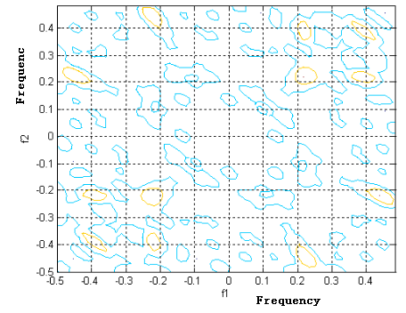
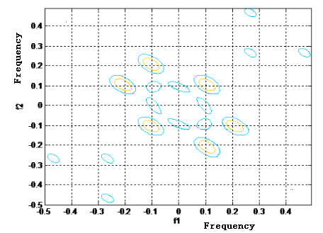
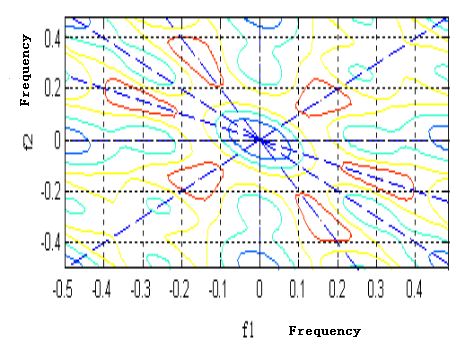
(a) Contour map of FLO bi-spectrum direct estimation method
(b) Contour map of FLO bi-spectrum indirect estimation method
(c) Contour map of FLO bi-spectrum estimation based on the AR model
Figure 1. Contour maps of the three methods
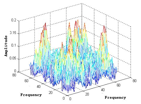
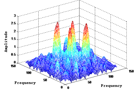
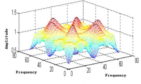
(a) 3D graph of FLO bi-spectrum direct estimation method
(b) 3D graph of FLO bi-spectrum indirect estimation method
(c) 3D graph of FLO bi-spectrum estimation based on the AR model
Figure 2. 3D graphs of the three methods
During the tests, the mixed noise ratio was set to -20dB, and the value of a to 1.5. The proposed method, the traditional nonparametric direct estimation method and the nonparametric indirect estimation method were all applied to the tests. The test results are displayed in Figures 1 and 2. As shown in Figures 1 and 2, the proposed method outperformed the traditional methods in signal identification and background noise suppression. In addition, our method managed to perverse the amplitude and phase information of the signal excellently, and achieve the best spectral flatness, laying the basis for the optimal whitening effect.
In practice, most background noises belong to the FLO, which cannot be suppressed well by traditional methods. In this paper, a FLO bi-spectrum estimation method is proposed based on the AR model, and new definitions are given for FLO three order cumulant. The author discussed the determination of AR model parameters, and introduced how to implement the bi-spectrum estimation method based on AR model. Then, a series of tests were performed to verify the correctness of our method. The results show that our method outperformed the traditional approaches in suppressing FLO noise and identifying relevant information of signals.
This work is supported by the Research Foundation of health department of Jiangxi Province (Grant No.20183016).
[1] Zha DF, Gao XY. (2006). Adaptive mixed norm filtering algorithm based on SαSG noise model. Journal on Communications 27(7): 1-6. https://doi.org/10.1016/j.dsp.2006.01.002
[2] Long JB, Wang HB. (2016). Parameter estimation and time-frequency distribution of fractional lower order time-frequency auto-regressive moving average model algorithm based on SaS process. Journal of Electronics & Information Technology 38(7): 1710-1716. http://dx.doi.org/10.11999/JEIT151066
[3] Spiridonakos MD, Fassois SD. (2014). Non-stationary random vibration modelling and analysis via functional series time-dependent ARMA (FS-TARMA) models – A critical survey. Mechanical Systems & Signal Processing 47(1): 175-224. https://doi.org/10.1016/j.ymssp.2013.06.024
[4] Madhavan N, Vinod AP, Madhukumar AS, Krishna AK. (2013). Spectrum sensing and modulation classification for cognitive radios using cumulants based on fractional lower order statistics. AEUE - International Journal of Electronics and Communications 67(6): 479-490. http://dx.doi.org/10.1016/j.aeue.2012.11.004
[5] Wang SY, Zhu XB, Li XT, Wang YL. (2007). A -spectrum estimation for AR SaS processes based on FLOC. Acta Electronica Sinica 35(9): 1637-1641. http://dx.chinadoi.cn/10.3321/j.issn:0372-2112.2007.09.004
[6] Qiu TS, Wang HY, Sun YM. (2004). A fractional lower-order covariance based adaptive latency change detection for evoked potentials. Acta Electronica Sinica 32(1): 91-95. http://dx.chinadoi.cn/10.3321/j.issn:0372-2112.2004.01.022
[7] Sun YM, Qiu TS, Wang FZ. (2003). Time delay estimation method of Non-stationary signals based on fractional lower spectrogram. Journal of Dalian Jiaotong University 37(3): 112-116.
[8] Liu JQ, Feng DZ. (2003). Blind sources separation in impulse noise. Journal of Electronics and Information Technology 31(12): 1921-1923.
[9] Feng Z, Liang M. (2013). Recent advances in time–frequency analysis methods for machinery fault diagnosis: A review with application examples. Mechanical Systems & Signal Processing 38(1): 165-205. https://doi.org/10.1016/j.ymssp.2013.01.017
[10] Liu GH, Zhang JJ. (2017). Fractional lower order cyclic spectrum analysis of digital frequency shift keying signals under the alpha stable distribution noise. Chinese Journal of Radio Science 32(1): 65-72. http://dx.chinadoi.cn/10.13443/j.cjors.2017011001
[11] Zha DF, Qiu TS. (2005). Generalized whitening method based on fractional order spectrum in the frequency domain. Journal of China Institute of Communications 26(5): 24-30.
[12] Shao M, Nikias CL. (1993). Signal processing with fractional lower order moments: stable processes and their applications. Proceedings of the IEEE 81(7): 986-1010. http://dx.doi.org/10.1109/5.231338
[13] Miller G. (1978). Properties of symmetric stable distribution. Journal of multivariate Analysis (8): 346-360.
[14] Xu B, Cui Y, Zhou UY. (2014). Unsupervised speckle level estimation of SAR images using texture analysis and AR model. IEICE Transactions on Communications 97(3): 691-698.
[15] Zhao N, Richard YF, Sun HJ. (2015). Interference alignment with delayed channel state information and dynamic AR model channel prediction in wireless networks. Wireless Net-works 21(4): 1227-1242. https://doi.org/10.1007/s11276-014-0850-7
[16] Cambanis S, Miller G. (1981). Linear problems in order and stable peicesses. SIAM Journal on Applied Mathematics 41(1): 43-69.
[17] Jiang YJ, Liu GQ, Wang TJ. (2017). Application of atomic decomposition algorithm based on sparse representation in AR model parameters estimation. Computer Science 44(5): 42-47.