Arnold Mauduit*![]() | Léa Salesse | Nicolas Bachelard | Hervé Gransac
| Léa Salesse | Nicolas Bachelard | Hervé Gransac
© 2025 The authors. This article is published by IIETA and is licensed under the CC BY 4.0 license (http://creativecommons.org/licenses/by/4.0/).
OPEN ACCESS
The study focuses on a 7000 series aluminium alloy (grade 7034), produced by melt spinning, a process based on the rapid solidification process (RSP). The aim of this process is to obtain a “nanostructured” material whose mechanical properties are improved through grain size refinement. This article addresses the influence of different heat treatments, in addition to the process itself, on the alloy's microstructure and mechanical properties. The aim of the study is therefore to provide a comparative metallurgical analysis of the alloy in different tempers (as extruded, T6 heat treated and annealed) using advanced observation methods (FEG-SEM, EDS, EBSD), physical tests (DSC, electrical conductivity) and mechanical tests (tensile and hardness tests). To establish the influence of heat treatment steps, this paper identifies the nature, size and distribution of the various alloy phases and determines the dislocation density and the grain size. It correlates the macroscopic mechanical behaviour with the microstructure, notably by establishing a direct relationship between the microstructure and the mechanical properties, thereby enabling the yield strength value to be predicted by determining the individual contribution of each alloy hardening mode: grain refinement (Hall-Petch equation), solid solution, density of geometrically necessary dislocations, and precipitation (JMAK model). Finally, it appears that the nanostructure contributes significantly to the overall hardening of the alloy and that it is greater than observed on 7000 series alloys produced by conventional processes.
nanostructured aluminium alloy, 7034, microstructure, mechanical properties
Aluminium alloys are of particular interest for their low density, good thermal and electrical conductivity and resistance to general corrosion, but they have (for most of them) static and dynamic mechanical properties that cannot compare with those of steels (featuring high mechanical properties) and titanium alloys. One way of increasing their mechanical properties is to apply the Hall-Petch equation and thus reduce their grain size, which implies the use of nanostructured alloys. The specificity of nanostructured alloys is that they have a nanoscale structure, i.e. a grain size less than 1µm.
Nanostructured aluminium alloys are mainly obtained by two methods: processes involving Severe Plastic Deformation (SPD) [1-3] and processes relying on rapid cooling of the material, usually at a rate greater than or equal to 106℃/s, also referred to as Rapid Solidification Processes (RSP) [4, 5].
Studies addressing the SPD method saw rapid development in the 2000s and 2010s, and mainly focused on the ECAP (Equal Channel Angular Pressing) process [6, 7]. Many studies have been conducted on the structural and mechanical changes induced in the 6061 alloy by ECAP processing [8-14]. More anecdotal processes, such as High Pressure Torsion (HPT), have also been studied alongside ECAP on the 6061 alloy [15]. Regarding the 7000 series alloys, ECAP was applied to the 7034 alloy to study its microstructural changes [16, 17]. Only a small number of companies currently use SPD processes to produce this type of alloy on an industrial scale. Honeywell Electronic Materials is the only company that uses the ECAP process on an industrial scale to produce targets for cathodic sputtering [18]. Recently, in 2020, Segal [19] proposed the industrial application of the Equal Channel Angular Extrusion (ECAE) process with a fairly precise concept and study. However, this process does not yet appear to have been adopted by industry.
The RSP method has found some use in industry with the melt spinning process [20, 21] applied by the RSP Technology company [22] to produce nanostructured aluminium alloys in the form of extruded bars [23]. The melt spinning process involves pouring a thin vertical stream of molten aluminium onto a copper wheel that rotates at high speed. The aluminium is cooled almost instantaneously and forms a continuous, nanostructured ribbon. The ribbon thus produced is chopped into “flakes” which are then compacted into billets which in turn are extruded into bars and profiles [22].
The aim of this document is to present the study of a nanostructured aluminium alloy produced using the RSP method. We chose the 7034 alloy offered by RSP Technology in an attempt to measure the contribution of the nanostructure (especially on mechanical properties) and highlight the relationships between the microstructure and the mechanical properties. In addition, as this alloy is also a structural hardening alloy, we will be able to look at all the hardening mechanisms involved: grain refinement strengthening, precipitation hardening, as well as solid solution hardening and strain hardening (dislocation density).
This type of nanostructured alloy has the potential to open aluminium alloys to industrial applications that are usually reserved for TA6V type titanium alloys, in other words to improve their strength-to-density and toughness-to-density ratios; and thus offer the 7034 alloy good prospects for applications in the manufacture of structural components for aeronautical and aerospace equipment.
2.1 Material and test specimens
RSP Technology provided us with two extruded bars (diameter 63.5mm-length 500mm-weight 9.2kg approximately) of nanostructured 7034 aluminium alloy in the following tempers:
- As extruded (AE)
- T6 (solution heat treated-quenched-artificially aged), hereinafter referred to as “T6f” (supplier-furnished T6)
All the tests and characterisations were carried out on test specimens (of various shapes) sampled from these two bars: discs, tensile test specimens, metallographic samples, etc.
The 7034 alloy belongs to the Al-Zn-Mg-Cu family. In general, this family of alloys offers high mechanical properties, making it interesting for applications in various sectors, such as aerospace or defence. In these alloys, Zn is mainly used to form hardening precipitates, while Cu and Mg contribute to the precipitation hardening and solid solution hardening mechanisms [24].
Several precipitation sequences have been observed in these alloys, depending on their compositions and the temperature of the precipitation hardening treatment. Four major intermetallic phases are expected in commercial Al-Zn-Mg-Cu alloys: the η phase (MgZn2 or Mg(Zn, Cu, Al)2 [25])-branch 1 (Figure 1); the T phase (Al2Zn3Mg3 or Mg3(Zn, Cu, Al)2 [26])-branch 2 (Figure 1); the S phase (Al2CuMg)-branch 3 (Figure 1); and the θ phase (Al2Cu)-branch 4 (Figure 1) [27].
Figure 1. Possible precipitation sequences in Al-Zn-Mg-Cu alloys [24]
The major precipitation sequence which prevails in the hardening of most commercially used 7000 series alloys corresponds to branch 1. For alloys with a Cu content <3 wt%, the θ phase does not appear [28]. Moreover, the precipitation sequence of branch 2 can be thermodynamically favoured by an Mg concentration >2 wt% [29]. Therefore, for the 7034 alloy (refer to Table 1), branches 1, 2 and possibly 3 are to be retained as possible precipitation sequences. Other intermetallic phases may appear in this type of alloy: Mg2Si (owing to the presence of Si in the alloy), and Al7Cu2Fe, a well-known intermetallic compound in 7000 series alloys which is undesirable as it reduces both the fatigue strength and toughness and promotes corrosion [30, 31].
The 7034 alloy was registered in 1999 in the “Teal Sheets” issued by The Aluminum Association [32].
2.2 Test and testing equipment
The chemical analyses were carried out using the ICP-AES method (Instrument: Hitachi FMP2) on two test specimens, the first one taken from the bar in AE temper, and the second one taken from the bar in T6f temper. The measurement uncertainties were calculated with a coverage factor equal to 2, which corresponds to a confidence interval of 95%.
The Brinell hardness measurements were carried out at room temperature with an EMCO-TEST Duramin 500 hardness tester (complying with standard EN ISO 6506-1). A minimum of three measurements were performed on every test specimen (only the average value is presented).
To measure the electrical conductivity of non-magnetic metals (as in the case of aluminium alloys), we relied on the eddy current testing technique. The instrument used was a Fischerscope MMS PC equipped with an ES40 probe, which itself was fitted with a thermocouple. In this configuration, the Fischerscope instrument instantaneously corrects the electrical conductivity as a function of temperature. We used a frequency of 60 kHz to ensure deep penetration into the alloy. At least three measurements were carried out per test specimen (only the average value is presented).
The samples for scanning electron microscopy were prepared in a conventional manner and examined using a JEOL JSM-IT800 FEG-SEM. This instrument is equipped with an Oxford Ultim Max 100 EDS (Energy Dispersive X-ray Spectroscopy) probe and an Oxford Symmetry EBSD (Electron Back Scattered Diffraction) camera. Note that the EBSD samples underwent a final polishing operation on a vibratory polishing machine (Presi Vibrotech 300 model). AztecCrystal 2.1 and Aztec 5.1 were used as operating software for EBSD and EDS mapping, respectively.
Differential Scanning Calorimetry (DSC) is a thermal analysis technique. It can measure differences in the heat exchanges between an analysed sample and a reference. The tests were carried out using a DSC Q2000 differential scanning calorimeter. For the working conditions, we selected a rate of temperature rise of 10°C/min over the range 25-550°C (under neutral nitrogen gas), in accordance with standard AITM 3-0008.
The tensile tests were carried out in accordance with standard ISO 6892-1, at room temperature and using a Zwick Z250 (250 kN) testing machine. The samples were taken from the extruded bars, in the longitudinal and transverse directions (in accordance with standard EN ISO 3785).
For heat treatment, the equipment used was a forced air convection oven. This oven is designed for aluminium alloy treatment (temperatures ≤650℃) and features excellent temperature homogeneity (ΔT≤6℃). The quenching fluid used is cold water (20℃ approximately). The time required to transfer the load (test specimens) into the quenching medium is less than 7 seconds in all circumstances (SAE standard AMS2772E).
The heat treatments applied to the 7034 alloy were as follows:
3.1 Chemical analysis
The results of the chemical analysis (Table 1) show that the chemical compositions of the two bars, AE and T6f, are almost identical (with a slight difference in the Mg content) and “almost” in line with grade 7034. Only the Si content is slightly outside the standardised range of the Teal Sheets. This does not call the alloy or its possible properties into question.
Table 1. Chemical analyses of the AE and T6f samples
|
|
Sample AE |
Sample T6f |
Expected Grade 7034 (Teal Sheets) |
|
Fe (wt%) |
0.095±0.011 |
0.095±0.011 |
≤0.12 |
|
Si (wt%) |
0.13±0.01 |
0.13±0.01 |
≤0.10 |
|
Cu (wt%) |
1.07±0.15 |
1.05±0.15 |
0.8–1.2 |
|
Zn (wt%) |
11.85±0.40 |
11.92±0.41 |
11.0–12.0 |
|
Mg (wt%) |
2.46±0.10 |
2.63±0.11 |
2.0–3.0 |
|
Mn (wt%) |
≤0.015 |
≤0.015 |
≤0.25 |
|
Ni (wt%) |
≤0.020 |
≤0.020 |
≤0.05 |
|
Cr (wt%) |
0.11±0.01 |
0.10±0.01 |
≤0.20 |
|
Ti (wt%) |
≤0.010 |
≤0.010 |
≤0.05 |
|
Pb (wt%) |
≤0.015 |
≤0.015 |
≤0.05 |
|
Sn (wt%) |
≤0.010 |
≤0.010 |
≤0.05 |
|
V (wt%) |
0.008±0.001 |
0.009±0.001 |
≤0.05 |
|
Zr (wt%) |
0.27±0.01 |
0.26±0.01 |
0.08–0.30 |
|
Al (wt%) |
Complement to 100% |
Complement to 100% |
Base |
3.2 Hardness and electrical conductivity testing
Electrical conductivity and conversely electrical resistivity are governed by the state of decomposition of the solid solution in the studied aluminium alloy. The room-temperature electrical conductivity measurement at is already used in the industrial world, particularly in the aerospace sector, as a quick and non-destructive method for checking the quenching and artificial aging of semi-finished products made of aluminium alloys.
Table 2 gives the hardness and electrical conductivity values for different tempers: AE and T6f provided by RSP Technology, and annealing (on AE and T6f tempers) carried out by us. We made no distinction between the annealing treatments on AE and T6f, as we found no differences.
Obviously, a higher hardness value can be noted for the T6f temper (precipitation hardened) and a low hardness value for the annealed temper. Conversely, electrical conductivity is always higher in the annealed temper, as the precipitates are incoherent with the aluminium matrix and therefore result in a less “impaired” current flow. The alloy seems to comply with RSP Technology’s specifications, which guarantee a minimum hardness of 205HB2.5/62.5 for the T6f temper.
Table 2. Hardness and electrical conductivity of different tempers
|
Tempers |
HBW 5/250 Brinell Hardness |
Electrical Conductivity (in MS/m) |
|
AE |
123.1±2.2 |
23.15±0.05 |
|
T6f |
205.5±2.6 |
18.49±0.07 |
|
Annealed (on AE and T6f) |
63.1±2.0 |
25.60±0.46 |
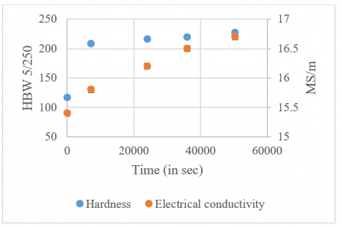
Figure 2. Changes in hardness and electrical conductivity during artificial aging at 120℃
In addition to annealing, we applied a solution heat treatment on the T6f and AE samples, followed by quenching and artificial aging between 2 hours and 14 hours at 120℃. The results are presented in Figure 2.
A sharp increase in the hardness value is observed after a simple artificial aging treatment of 2 hours at 120℃, compared to the “as quenched” temper. The hardness then stabilises and tends towards a maximum. After 14 hours at 120°C, the hardness reaches approximately 227HBW5/250, i.e. a value markedly higher than that of the sample supplied in T6 temper (205.5HBW5/250). Also note that the electrical conductivity after 14 hours at 120℃ is lower (16.7MS/m) than that found on the T6f temper supplied. This may suggest that the T6f temper supplied by RSP Technology shows a tendency to over-aging: lower hardness and higher electrical conductivity than a possible optimum at 227HBW5/250 and 16.7MS/m.
The study of the precipitation kinetics is associated with the nucleation and growth processes which are predominant in supersaturated aluminium alloys. The kinetics of isothermal phase transformation through nucleation and growth are often described by the Johnson-Mehl-Avrami-Kolmogorov (JMAK) model [33] which postulates that nucleation occurs randomly and that growth is homogenous.
The JMAK model is based on the concept of an “extended volume” which is the volume that a new nucleus would occupy if there was no encroachment or overlapping of an already transformed adjacent nucleus [33-37].
The JMAK model equation is:
$x(t)=1-\exp \left(-[k(T) t]^n\right)$ (1)
where,
$x(t)$ is the transformed volume fraction.
$n$ is the Avrami exponent which reflects the transformation mechanism.
$t$ is the isothermal holding time.
$k(T)$ is a rate constant which primarily depends on the temperature and which may be expressed by an Arrhenius equation:
$k(T)=k_0 \exp \left(-\frac{E_a}{R T}\right)$ (2)
where, $E_a$ is the activation energy for the nucleation and isothermal growth, $k_0$ is a constant and $R$ is the universal gas constant.
The transformed volume fraction at time $\mathrm{t}: x(t)$ may b obtained from the electrical conductivity measurement presented using the Eq. (4) below. Following this, parameters ( $n$ and $k(T)$ ) of the JMAK model can determined based on Eq. (1) as follows [33]:
$\ln \left(\ln \left(\frac{1}{1-x(t)}\right)\right)=n \ln t+n \ln (k(T))$ (3)
The transformed volume fraction in an isothermal reaction can be described as follows [38, 39]:
$x(t)=\frac{\sigma(t)-\sigma_0}{\sigma_f-\sigma_0}$ (4)
where,
$x(t)$: transformed volume fraction at time t (isothermal transformation)
$\sigma(t)$: electrical conductivity at time t
$\sigma_0$: initial electrical conductivity
$\sigma_f$: final electrical conductivity
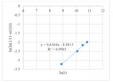
Figure 3. Validation and determination of the parameters of the JMAK model
Figure 3 implements the approach for the JMAK model and we can see that that we obtain a straight line with good linear regression, which validates the fact that the kinetics follows the JMAK model (Eq. (3)). Therefore, we obtain $n$=0.6364 and $k(T)$=8.69.10-7. It is possible to associate the Avrami exponent ($n$) with a precipitation morphology during an isothermal transformation; here the Avrami exponent is close to the 2/3 value which is well known to correspond to a mechanism of precipitation on dislocations with diffusion-controlled growth [39]. The JMAK model therefore appears to be validated and these parameters determined.
3.3 Metallurgical examinations
For these examinations, which are mainly FEG-SEM, EDS and EBSD observations, we used 4 samples taken from the extruded bars in AE and T6f tempers. The samples identified as -1 and -2 were taken perpendicular to the direction of extrusion, while the samples identified as ‑3 and ‑4 were taken along the direction of extrusion. Note that samples ‑1 and ‑3 were taken from the core of the bar, while samples ‑2 and ‑4 were taken from the edge of the bar.
3.3.1 Microstructure and grain size
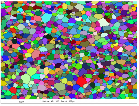
The first EBSD observations reveals a fine-grained structure for all samples. For example, Figure 4, which presents the microstructure of the T6f temper (T6f sample No. ‑2), highlights a fine, equiaxed grain structure. A more detailed analysis of the grain map shows the following:
Figure 4. EBSD observation on T6f sample No. -2 (supplier-furnished). Grain map (in random colours) and grain boundaries (threshold angle 10°)
This fine-grained structure is explained by the extremely high cooling rate (106℃/s) of the RSP process. Indeed, during rapid solidification, the material quickly changes from the liquid to the solid state. This rapid transition favors the formation of many nucleation sites (where grains begin to form) because a high cooling rate provides a strong driving force for the nucleation process [40]. The more nucleation sites there are, the smaller the grains will be. In addition, the high cooling rate limits the time available for grain growth; the grains do not have enough time to reach a large size before the material is completely solidified.
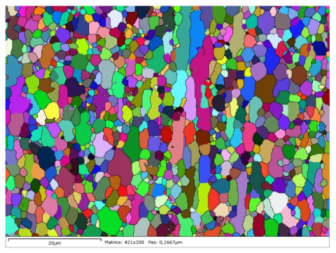
During the extrusion operation, it is common to observe a wrought effect in the aluminium alloy: this is the press effect, i.e. an orientation of the grains (elongated grains) in the direction of extrusion which, for our samples, should be visible on samples No.‑3 and No.‑4. For the AE temper, the direction of extrusion is clearly shown by grains oriented along that direction (on AE samples No.‑3 or No.‑4), whereas this orientation is much less present in the T6f temper. All the grains are rather equiaxed, even in T6f samples No.‑3 and No.‑4 (example in Figure 5). As a matter of fact, Figure 5 (a) shows AE sample No.‑3, where (clearly marked) zones of elongated grains oriented in the direction of extrusion are intersected with zones of fine and rather equiaxed grains. On T6f sample No.‑3 (Figure 5 (b)), however, it is more difficult to distinguish zones of elongated grains, while zones of fine and equiaxed grains are observed instead. We can also note that the grains are finer in AE sample No.‑3 than in T6f sample No.‑3.
(a) AE sample No.‑3.
(b) T6f sample No.‑3.
Figure 5. EBSD observations – Grain map (in random colours) and grain boundaries (threshold angle 10°)
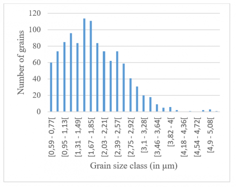
In addition, not all grains are smaller than one micrometre, which raises the question of the alloy’s nanostructure. Figure 6 shows the equivalent-circle diameter distribution on the example of the EBSD grain map of Figure 4 (T6f sample No.‑2). It appears that only 14% of the grains (out of a total of 1,116) have a grain size smaller than one micrometre. Under such conditions, can this alloy be considered nanostructured? To complete the picture, note that 63.5% of the grains feature a size smaller than 2µm, which is in line with the average of 1.84µm (previously observed).
Figure 6. Grain size distribution according to the equivalent circle diameter – “Grain size” on T6f sample No.‑3 (supplier-furnished)
To check the homogeneity of the material in the T6f and AE tempers, Table 3 groups together the essential results of all the observations making it possible to compare the samples. This leads to the findings below:
The difference in grain size and proportion of nanostructure between the T6f and AE tempers can potentially be explained by some homogenisation and slight grain coarsening during the solution heat treatment applied to obtain the T6f temper. It is also worth noting that, in the T6f temper, samples No.‑1 and No.‑2 are similar in terms of nanostructure proportion (approximately 14% to 15%), as are samples No.‑3 and No.‑4 (approximately 19%), which means that the sampling direction seems to affect the proportion of grains ≤1µm. This is not the case with the AE temper, where it appears that the difference is more pronounced between the core and the edge of the extruded bar (samples No.‑1 and No.‑3 taken from the core of the bar, and samples No.‑2 and No.‑4 taken from the edge of the bar).
According to the work of Starink et al. [16, 17] on the 7034 alloy produced using the ECAP process, the grain size stabilises at approximately 0.5µm after 4 passes. Compared to the grain sizes observed after the RSP process (followed by extrusion), i.e. the AE temper, this value is markedly lower: approximately 3 times smaller. And in this case, the alloy is considered nanostructured without difficulty.
Table 3. “Grain size” data obtained from EBSD observations
|
EBSD Grain Map Identification |
Mean Equivalent Circle Diameter (in µm) |
Maximum Equivalent Circle Diameter (in µm) |
Proportion of Grains ≤1µm (in%) |
|
T6f -1 |
1.72 |
5.39 |
15 |
|
T6f -2 |
1.84 |
5.08 |
14 |
|
T6f -3 |
1.85 |
8.23 |
19.5 |
|
T6f -4 |
1.9 |
6.03 |
19 |
|
AE -1 |
1.39 |
5.99 |
33 |
|
AE -2 |
1.52 |
4.15 |
23.5 |
|
AE -3 |
1.47 |
11.87 |
37.5 |
|
AE -4 |
1.75 |
5.49 |
21.5 |
When we applied a new T6 temper, thus identified as T6c, we did not notice any particular changes in the microstructure, compared to the T6f temper: the grain size remained comparable (on average close to 2µm for the mean equivalent circle diameter), and the proportion of grains ≤1µm remained the same as that of the T6f temper (around 14% to 15%).
(a) Low magnification, 400X
(b) High magnification, 3500X, with EDS analysis to identify the phases
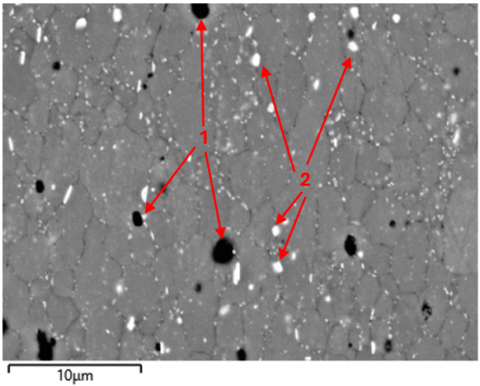
Figure 7. AE temper-FEG-SEM observations in BED mode
3.3.2 Precipitation and intermetallic compounds
In this chapter, the aim is to observe and determine the precipitations and intermetallic compounds in 4 tempers: AE, T6f, T6c and annealed.
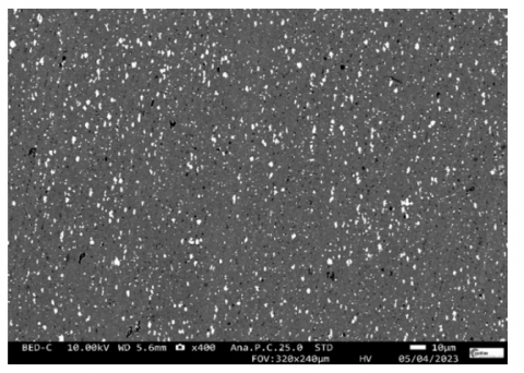
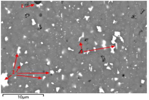
In the AE temper, many precipitates are visible, as shown in Figure 7 which is obtained through FEG-SEM examination in backscattered electron mode (BED). It highlights the phase contrast: atoms with a high atomic number appear brighter. The precipitates can be broken down into two major families, those with “heavy”, i.e. bright, atoms, and those with “light”, i.e. dark, atoms. The AE temper features a rather high density of uniformly distributed, fragmented precipitates (smaller than 5µm). In Figure7 (b), the EDS analysis was used, leading to the following findings:
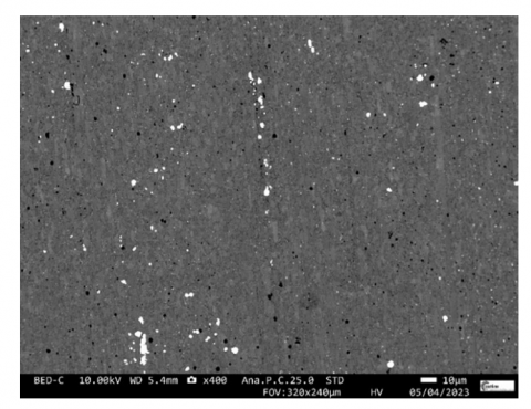
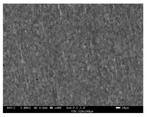
In the T6f temper, we used the same approach as above and obtained Figure 8. A lower density of precipitates can be noted, in particular for brighter precipitates, i.e. those with “heavy” atoms. This can be explained easily by the fact that a certain quantity of elements were put back into solution with the T6 heat treatment (during the solution heat treatment phase). As before, using the EDS method on Figure 8 (b), we found that:
Therefore, this confirms that the η phase (Mg(Zn, Cu, Al)2) and/or the T phase (Mg3(Zn, Cu, Al)2) was/were put back into solution.
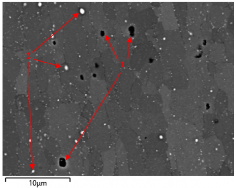
Note that in the T6c temper (re-solution heat treatment carried out by Cetim), the density of precipitates appears to be even lower than in the T6f temper, along with the presence of finer precipitates. This implies better re-solution of the various phases (Figure 9), in particular the Al7Cu2Fe intermetallic compounds. As before, the findings are as follows:
(a) Low magnification, 400X
(b) High magnification, 3500X, with EDS analysis to identify the phases
Figure 8. T6f temper-FEG-SEM observations in BED mode
(a) Low magnification, 400X
(b) High magnification, 3500X, with EDS analysis to identify the phases
Figure 9. T6c temper-FEG-SEM observations in BED mode
This better re-solution certainly has an impact on the mechanical properties and electrical conductivity of the alloy, and may partly explain the differences in hardness and electrical conductivity observed in § 3.2 between the T6f and T6c tempers.
We examined the T6f temper at higher magnification in an attempt to understand the hardening precipitation of the η’ and T’ phases (refer to § 2.1). Figure 10 shows fine precipitation, approximately 10nm to 20nm in diameter, but with our equipment (FEG-SEM and EDS), we are not in a position to identify these phases. However, with an image processing software program, it becomes possible to isolate the fine bright precipitates through thresholding and determine their sizes (diameters) by working out the average on a large number of precipitates. In the example shown in Figure 10, this method gives an average diameter of 14±4nm. In the literature, it has been shown that the Zn/Mg ratio has an influence on the microstructure and precipitation of alloys from the Al-Zn-Mg-Cu family [41]. For example, for equivalent alloys with comparable Zn/Mg ratios (i.e. around 4.7 in our case), the precipitates in the T6 temper range from 4nm to 8nm in diameter [42-44]. Zou et al. [41] also report that, for this type of Zn/Mg≈4.5 alloy, the T’ and η’ precipitates are found in almost equal proportions with, in particular for their study, diameters of 4.6±1.0nm for the T’ phase and 6.4±1.4nm for the η’ phase. When the alloy reaches an over-aged state towards the T7 temper, the precipitates grow. Wen et al. [43] report that the precipitates in the Al-Zn-Mg-Cu alloys reach diameters of up to 20nm for the T73 temper. The diameters of precipitates measured in our study for the 7034 alloy in T6f temper appear somewhat larger than those found in the literature for alloys from the same family. Thus, the size of the precipitates would be more consistent with a slightly over-aged temper, as mentioned in § 3.2, where we explain that a higher electrical conductivity and a lower hardness than a potential optimum (noted T6c) may suggest an over-aged temper.
Figure 10. T6f temper-FEG-SEM observation. Fine precipitation
Figure 11. T6c temper-FEG-SEM observation. Precipitation bands framed by red dotted lines
Occasionally, a non-uniform distribution of precipitation was observed in the T6 temper (especially T6c) in the form of bands, as shown in Figure 11. According to Deschamps [45], the heterogeneous distribution of dispersoids leads to heterogeneous precipitation distribution.
(a) Annealed temper obtained after an initial T6 temper, low magnification (400X)
(b) Annealed temper obtained after an initial AE temper, low magnification (400X)
(c) High magnification (3500X) with EDS analysis to identify the phases
Figure 12. FEG-SEM observations in BED mode
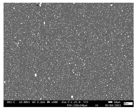
In the annealed temper, the microstructure differs depending on the initial temper applied before annealing (Figure 12). In fact, starting from the T6 temper, the numerous precipitates are homogeneously distributed in size and volume (Figure 12 (a)), which is not the case when starting from the AE temper where the precipitates are coarser and more heterogeneously distributed (Figure 12 (b)). As before, an EDS analysis leads to the following findings:
Again, there are no signs of S-type precipitates.
3.3.3 Strain hardening and dislocations
We studied the strain hardening of the 7034 alloy in the T6f, AE and annealed tempers, using the EBSD observations. In fact, with the Kernel Average Misorientation (KAM), it is possible to obtain the density of geometrically necessary dislocations (GND), noted $\rho_{G N D}$. The KAM, which expresses the local misorientation, is linked to the density of geometrically necessary dislocations $\rho_{G N D}$ by the following equation:
$\rho_{G N D}=\frac{\alpha \cdot \Delta \theta}{b \cdot \Delta x}$ (5)
This is Ashby’s equation [46] which relates the curvature of the crystal lattice $\frac{\Delta \theta}{\Delta x}$ to the density of geometrically necessary dislocations.
where,
$\alpha$ is a constant between 1 and 5 (depending on the configuration)
$\Delta \theta$ is the misorientation of the lattice, that is to say the KAM
$\Delta x$ is the size of the kernel (or the pitch)
$b$ is the Burgers vector (for aluminium: 0.286nm <110> [24, 45])
The EBSD technique only allows obtaining the geometrically necessary dislocation density (GND) and does not provide information on the total dislocation density which is made up of the density of geometrically necessary dislocations and statistically stored dislocations.
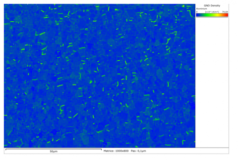
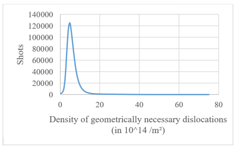
(a) Representation in map format
(b) Distribution of the GND densities
Figure 13. T6f temper-GND density from EBSD observations
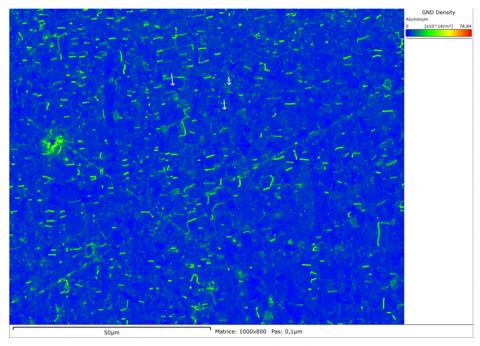
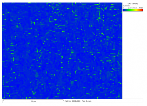
(a) AE temper
(b) Annealed temper
Figure 14. GND density from EBSD observations
Figure 13 (a) shows, in a “thermal” map format, the density of geometrically necessary dislocations $\rho_{G N D}$ in the T6f temper. Note that the density is finally rather low and localised at the grain boundaries. Figure 13 (b) shows the distribution of this density and provides a weighted average: a value of 6.22×10¹⁴/m² is obtained, which can be associated with the $\rho_{G N D}$ value of the alloy in the T6f temper.
Figure 14 presents the GND density maps for the AE temper (Figure 14 (a)) and the annealed temper (Figure 14 (b)). It can be seen that the values are comparable (AE, annealed and T6f tempers): they show very little difference. The GND density is rather low and the dislocations are located at the grain boundaries. Note that the weighted average is $\rho_{G N D}$=5.49×10¹⁴/m² in the AE temper, and $\rho_{G N D}$=4.02×10¹⁴/m² in the annealed temper. Therefore, the weighted average GND density follows a logical order of tempers: T6f >AE >annealed. As a matter of fact, the T6f temper, owing to the quenching operation, can potentially feature a slightly higher GND density level, whereas the annealed temper obviously has the lowest level due to softening of the alloy.
3.4 Differential scanning calorimetry (DSC) tests
With these tests, some of the microstructural changes of aluminium alloys can be determined, such as phase transformations: exothermic transformation for precipitation, and endothermic transformation for dissolution or melting.
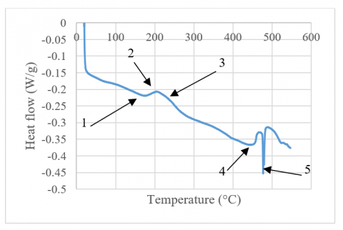
Figure 15 presents the DSC curve for the T6f temper. Note the three endothermic valleys or peaks, identified as 1, 4 and 5 and the 2 exothermic peaks, identified as 2 and 3. According to the literature on this topic [16, 24, 28, 45, 47], we can attribute:
The DSC analysis confirms the presence of the η and T phases, which were imperceptible in the EDS analysis (refer to § 3.3.2). Therefore, as previously indicated by [41], it is very likely that both η’ and T’ phases coexist.
Figure 15. T6f temper-DSC curve
3.5 Mechanical properties
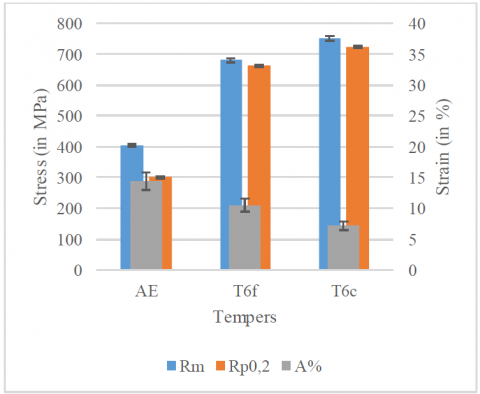
Figure 16 presents the mechanical properties of the RSP 7034 alloy, in three different tempers: T6c, T6f and AE, in the longitudinal direction of the procured bar.
The following can be noted (Figure 16 (a)):
(a) Comparison of Rm, Rp0.2 and A%
(b) Conventional curves
Figure 16. Mechanical properties of the RSP 7034 alloy, longitudinal direction
The Rm, Rp0.2 and A% values obtained in the T6f temper of the RSP 7034 alloy (after extrusion) can be compared to those presented by Samant et al. [48] for spray-cast samples of 7034 alloy treated to T6 temper (after extrusion). The values are close but slightly lower for the T6f temper: Rm=696.4MPa for [48] and 680MPa for our study; Rp0.2 =679.2MPa for [48] and 661MPa for our study; and A=11.7% for [47] and 10.5% for our study. This can confirm a tendency of the T6f temper towards over-aging.
Figure 16 (b) shows examples of conventional stress-strain curves for the AE, T6f and T6c tempers. Note that the curves of the T6 temper have the usual morphology of this temper, i.e. a significant tendency towards perfect elastoplasticity. This is reflected by the strain hardening coefficient n which is “almost” zero. In the T6c temper, this coefficient is around 0.018, and only 0.011 for the T6f temper. In contrast, the AE temper features a higher strain hardening coefficient n of 0.173.
(a) Low magnification: intergranular cracking
(b) High magnification: presence of dimples
Figure 17. T6f temper. Observations of the fracture surface of a tensile test specimen
It can also be noted that the mechanical strength-to-density ratio (or specific strength) is close to the typical value for TA6V titanium alloys. As a matter of fact, the best ratio is around 265 for a TA6V alloy, 235 for the 7034 aluminium alloy in the T6f temper, and even 259 for the T6c temper.
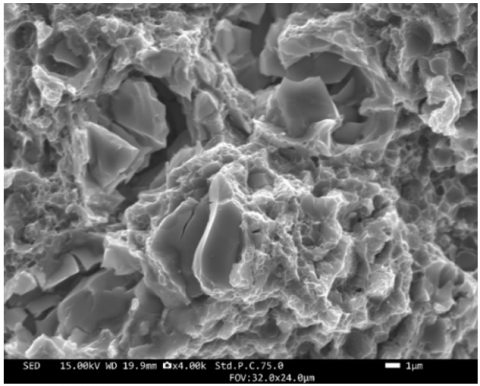
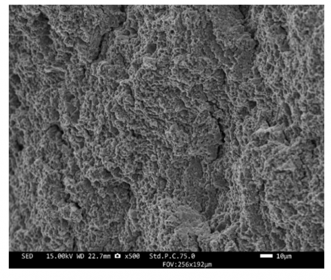
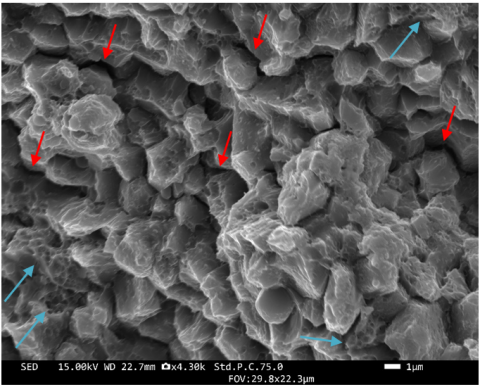
Despite an elongation value in excess of 10% in the T6f temper, the fracture surfaces of the tensile test specimens exhibit intergranular cracks (Figure 17 (a)). At high magnification (Figure 17 (b)), fine dimples are visible on the surface of the grains, which is, however, indicative of the ductile nature of the fracture. In the T6c temper, the same intergranular cracks can be seen on the fracture surfaces of the tensile test specimens (Figure 18 (a)). However, at higher magnification (Figure 18 (b)), the intergranular nature of the fracture is still very much visible. The small-sized grains are clearly visible, sometimes with intergranular cracks (red arrows). The areas with fine dimples (blue arrows) are relatively rare compared to the T6f temper. Therefore, both T6 tempers, but more markedly for the T6c temper, exhibit what Zou et al [41] call the “rock candy” effect, which shows the brittle nature of the intergranular fracture of the RSP 7034 alloy.
(a) Low magnification: intergranular cracking
(b) High magnification: “rock candy” appearance
Figure 18. T6c temper. Observations of the fracture surface of a tensile test specimen
In view of the characterisations previously carried out and described in § 3, we are now in a position to analyse the relationships between the microstructure and the mechanical properties, i.e. establish a correlation between the mechanical behaviour and the microstructure. In the remaining part of this study, we will take the particular example of the T6f temper (potentially showing a tendency towards over-aging) which is representative of the RSP 7034 alloy and the procurable semi-finished products.
The idea is to calculate the various contributions of the microstructure to the hardening mechanisms of the alloy in the T6f temper, and more specifically to the yield strength. The hardening mechanisms identified are listed below:
4.1 Contribution of grain size to the yield strength
As previously mentioned, the relationship which connects the grain size and the yield strength $\left(\sigma_e\right)$ is the Hall-Petch equation [49]:
$\sigma_{e G B}=\sigma_0+\frac{k}{\sqrt{d}}$ (6)
where,
$\sigma_{e G B}$ is the contribution of grain refinement strengthening to the yield strength.
$\sigma_0$ is the friction stress.
$k$ is the Hall-Petch slope.
$d$ is the average grain diameter.
For alloys of the $\mathrm{Al}-\mathrm{Zn}-\mathrm{Mg}-\mathrm{Cu}$ family, $\sigma_0=16 \mathrm{MPa}$ [49] and $k=0.12 \mathrm{MPa} \sqrt{m}$ [50, 51]. The experimental parameter that needs to be determined is the average grain diameter (i.e. the grain size): $d$. The average value of $d$ is $1.82 \mu \mathrm{~m}$, given by T6f samples Nos.-1 to -4 and presented in Table 3, para 3.3.1. This gives: $\sigma_{\rho G B}=105 \mathrm{MPa}$.
4.2 Contribution of solid solution hardening to the yield strength
The effect of solid solution hardening on the yield strength was studied by Myhr et al. [52] and can be defined as follows:
$\sigma_{e s s}=\sum_i K_i C_i^{2 / 3}$ (7)
where,
$\sigma_{e s s}$ is the contribution of solid solution hardening to the yield strength
$C_i^{2 / 3}$ is the concentration of element i in the alloy, expressed in % by mass
$K_i$ is a hardening constant related to element i
In our case, $K_{Z n}=2.9 \mathrm{MPa}, K_{M g}=18.6 \mathrm{MPa}$ and $K_{C u}=13.8 \mathrm{MPa}$, according to the study [53]. The experimental parameters that need to be determined are the concentrations of elements Zn, Mg and Cu (% by mass).
When all elements are in a solid solution (a situation which is not certain in practice but possible in theory and would correspond to an "as quenched" condition), then $\sigma_{\text {ess }}=64.8 \mathrm{MPa}$ using the chemical composition given in Table 2. Now, assuming a state of equilibrium at room temperature (which would correspond to an annealed temper), we use $C_{Z n}=1 \%, C_{M g}=1.7 \%$ and $C_{C u}=0.05 \%$, that is to say the limiting solubility values (\% by mass) at room temperature in the state of equilibrium [54]; we then obtain $\sigma_{\text {ess }}=31.3 \mathrm{MPa}$. Thus, the $\sigma_{e s s}$ value in the T6f temper ranges between these two values. To continue our demonstration, we choose an arbitrary value that corresponds to the average of the two previous cases, i.e. 48 MPa .
4.3 Contribution of structural hardening to the yield strength
In this situation, two cases arise.
The precipitates are shearable, and we use the equation of the studies [55-57]:
$\sigma_{e p}=\sqrt{\frac{3}{4 \pi \beta}} \frac{k_p^{3 / 2} M \mu}{\sqrt{b}} \sqrt{f_v R}$ (8)
where,
$\sigma_{e p}$ is the contribution of precipitation hardening (case of shearable precipitates) to the yield strength
$M$ is the Taylor factor
$\mu$ is the shear modulus
$b$ is the Burgers vector
$f_v$ is the volume fraction of precipitates
$R$ is the average precipitate radius
$\beta=0.43$ and $k_p=0.07$ according to the study [58] ; M=3.06 [24, 44], $\mu=26.9 \mathrm{MPa}$ [24, 45], $b=0.286 \mathrm{~nm}$ [24, 45]. The experimental parameters that need to be determined are the volume fraction of precipitates and the average precipitate radius.
The precipitates can be bypassed; thus we have the equation of the studies [57, 59]:
$\sigma_{e p}=0.6 M \mu b \frac{\sqrt{f_v}}{R}$ (9)
where,
$\sigma_{e p}$ is the contribution of precipitation hardening (case of shearable precipitates) to the yield strength
$M$ is the Taylor factor
$\mu$ is the shear modulus
$b$ is the Burgers vector
$f_v$ is the volume fraction of precipitates
$R$ is the average precipitate radius
And $M$=3.06 [24, 45], $\mu$=26.9MPa [24, 45], b=0.286nm [24, 45]. Again, the experimental parameters that need to be determined are the volume fraction of precipitates and the average precipitate radius.
The transition from shear to bypass occurs at a critical precipitate radius [45]:
$R_c=0.9 \frac{b}{\alpha}$ (10)
where,
$R_c$ is the critical precipitate radius
$b$ is the Burgers vector
$\alpha$ is a constant representing the strength of the obstacle [45]
For aluminium alloys, $\alpha \approx 0.1$ [45], hence $R_c=2.574 \mathrm{~nm}$. Thus, considering the average radius of measured precipitates, i.e. 7 nm (refer to § 3.3.2), the precipitates can be bypassed, so we use Eq. (9). We then need to determine the precipitate volume fraction in the T6f temper; for that purpose, we use the JMAK model and the transformed volume fraction Eq. (4) (refer to § 3.2). Hence, for $\sigma(t)=18.49 \mathrm{MS} / \mathrm{m}$ (T6f temper), we obtain $f_v=0.055$. This gives $\sigma_{e p}=473 \mathrm{MPa}$.
4.4 Contribution of strain hardening or dislocations to the yield strength
In this case, the corresponding strain hardening in the yield strength can be estimated with the Bailey-Hirsch relationship [60]:
$\sigma_{e d i s}=M \chi \mu b \sqrt{\rho}$ (11)
where,
$\sigma_{\text {edis }}$ is the contribution of strain hardening to the yield strength
$\chi$ is the Taylor factor
χ is a constant related to the material
$\mu$ is the shear modulus
$b$ is the Burgers vector
$\rho$ is the dislocation density
For aluminium alloys, $M=3.06, \mu=26.9 \mathrm{MPa}, b=0.286 \mathrm{~nm}$, $\chi=0.27$ [61]. The experimental parameter that needs to be determined is the dislocation density, i.e. the $\rho_{G N D}$ value measured in § 3.3.3. Hence, $\sigma_{\text {edis }}=159 \mathrm{MPa}$. It should be noted that we considered that $\sigma_{\text {edis }}$ was essentially due to $\rho_{G N D}$. For the first moments of plasticity or for the end of elasticity (yield limit zone), the contribution of $\rho_{G N D}$ to hardening is the most important [62].
4.5 Total contribution to the yield strength and analysis
There are various ways of adding together the contributions to the yield strength, especially when obstacles of identical strength but different densities are present. In this case, we use the Deschamps model [58]:
$\sigma_{\text {etotal }}=\sigma_{e G B}+\sigma_{e s s}+\sqrt{\sigma_{e p}^2+\sigma_{e d i s}^2}$ (12)
This gives $\sigma_{etotal}$ =652MPa, a value which can be compared to the average Rp0.2 of the T6f temper (refer to § 3.5), which is 661MPa. A slight difference can be noted (less than 1.5%) between the two values. This can be explained in many ways, but in particular by the value of $\sigma_{e s s}$ which remains rather inaccurate in our study (48MPa chosen, but ranging between 31.3MPa and 64.8MPa). It can be concluded that the mechanical properties and the microstructure are correlated, or that the microstructure can allow the mechanical properties to be predicted: relationship between microstructure and mechanical properties.
Unsurprisingly, precipitation hardening is predominant. However, the contribution of the nanostructure to overall hardening is significant and far superior than in “conventional” aluminium alloys. For example, when compared to wrought aluminium alloys from the same family where the grain size (equivalent circle diameter) is of the order of 10µm to 50µm, the $\sigma_{e G B}$ contribution obtained amounts only to 30MPa to 50MPa, i.e. 2 to 3 times lower.
In addition, we can use the elements that we have already obtained to determine the total contribution of hardening to the yield strength for the AE temper. In view of the electrical conductivity of the AE temper, we can consider that this temper is close to the annealed temper in terms of precipitation and elements in solid solution. Therefore, we consider that $\sigma_{e p}$ is low and even close to 0 , and that $\sigma_{e s s}=31.3 \mathrm{MPa}$ (refer to § 4.2). Furthermore, $\sigma_{e G B}=113 \mathrm{MPa}$ (Hall-Petch equation with a grain size of $1.53 \mu \mathrm{~m}$ (refer to Table 3)) and $\sigma_{\text {edis }}=149 \mathrm{MPa}$ (refer to § 3.3.3). Thus we obtain $\sigma_{\text {etotal }}=293 \mathrm{MPa}$, a value which is to be compared to the 300 MPa presented in Figure 16. Bearing in mind that we slightly underestimate $\sigma_{e p}$ and $\sigma_{e s s}$, the result obtained is consistent.
The approach developed previously fairly accurately reflects the mechanical characteristics of the nanostructured 7034 alloy in the T6f and AE temper. This tool can be considered to predict the mechanical properties of nanostructured aluminium alloys and therefore to adapt them to specific applications. This statement is qualified by the difficulty of knowing how to implement the right "metallurgy" to obtain the right grain size or the right dislocation density, for example.
We were able to characterise the RSP 7034 alloy in several tempers:
Note that, using relatively accessible analysis techniques, we were able to demonstrate the following:
With these analyses, we achieved the objective of establishing a correlation between the microstructure and the mechanical properties. To that end, we relied on current knowledge to implement the approach aimed at determining the contribution of each type of hardening to the yield strength.
The authors wish to thank CETIM (Centre Technique des Industries de la Mécanique - Technical Centre for the mechanical industries) for the funding and support provided for this study.
[1] Lowe, T.C., Valiev, R.Z. (2012). Investigations and applications of severe plastic deformation. Springer Science & Business Media, Vol. 80. https://doi.org/10.1007/978-94-011-4062-1
[2] Valiev, R.Z., Islamgaliev, R.K., Alexandrov, I.V. (2000). Bulk nanostructured materials from severe plastic deformation. Progress in Materials Science, 45(2): 103-189. https://doi.org/10.1016/s0079-6425(99)00007-9
[3] Zehetbauer, M.J., Valiev, R.Z. (Eds.). (2006). Nanomaterials by severe plastic deformation. John Wiley & Sons.M. https://doi.org/10.1002/3527602461
[4] Lavernia, E., Rai, G., Grant, N.J. (1986). Rapid solidification processing of 7xxx aluminium alloys: A review. Materials Science and Engineering, 79(2): 211-221. https://doi.org/10.1016/0025-5416(86)90406-4
[5] Lavernia, E.J., Ayers, J.D., Srivatsan, T.S. (1992). Rapid solidification processing with specific application to aluminium alloys. International Materials Reviews, 37(1): 1-44. https://doi.org/10.1179/imr.1992.37.1.1
[6] Furukawa, M., Horita, Z., Nemoto, M., Langdon, T.G. (2002). The use of severe plastic deformation for microstructural control. Materials Science and Engineering: A, 324(1-2): 82-89. https://doi.org/10.1016/s0921-5093(01)01288-6
[7] Valiev, R.Z., Langdon, T.G. (2006). Principles of equal-Channel angular pressing as a processing tool for grain refinement. Progress in Materials Science, 51(7): 881-981. https://doi.org/10.1016/j.pmatsci.2006.02.003
[8] Ferrasse, S., Segal, V.M., Hartwig, K.T., Goforth, R.E. (1997). Development of a submicrometer-grained microstructure in aluminum 6061 using equal channel angular extrusion. Journal of Materials Research, 12(5): 1253-1261. https://doi.org/10.1557/jmr.1997.0173
[9] Kim, J.K., Jeong, H.G., Hong, S.I., Kim, Y.S., Kim, W.J. (2001). Effect of aging treatment on heavily deformed microstructure of a 6061 aluminum alloy after equal channel angular pressing. Scripta Materialia, 45(8): 901-907. https://doi.org/10.1016/s1359-6462(01)01109-5
[10] Kim, W.J., Kim, J.K., Park, T.Y., Hong, S.I., Kim, D.I., Kim, Y.S., Lee, J.D. (2002). Enhancement of strength and superplasticity in a 6061 Al alloy processed by equal-channel-angular-pressing. Metallurgical and Materials Transactions A, 33: 3155-3164. https://doi.org/10.1007/s11661-002-0301-4
[11] Kim, J.K., Kim, H.K., Park, J.W., Kim, W.J. (2005). Large enhancement in mechanical properties of the 6061 Al alloys after a single pressing by ECAP. Scripta Materialia, 53(10): 1207-1211. https://doi.org/10.1016/j.scriptamat.2005.06.014
[12] Chaudhury, P.K., Cherukuri, B., Srinivasan, R. (2005). Scaling up of equal-Channel angular pressing and its effect on mechanical properties, microstructure, and hot workability of AA 6061. Materials Science and Engineering: A, 410: 316-318. https://doi.org/10.1016/j.msea.2005.08.023
[13] Kim, W.J., Wang, J.Y. (2007). Microstructure of the post-ECAP aging processed 6061 Al alloys. Materials Science and Engineering: A, 464(1-2): 23-27. https://doi.org/10.1016/j.msea.2007.03.074
[14] Chung, C.S., Kim, J.K., Kim, H.K., Kim, W.J. (2002). Improvement of high-Cycle fatigue life in a 6061 Al alloy produced by equal channel angular pressing. Materials Science and Engineering: A, 337(1-2): 39-44. https://doi.org/10.1016/s0921-5093(02)00010-2
[15] Nurislamova, G., Sauvage, X., Murashkin, M., Islamgaliev, R., Valiev, R. (2008). Nanostructure and related mechanical properties of an Al-Mg-Si alloy processed by severe plastic deformation. Philosophical Magazine Letters, 88(6): 459-466. https://doi.org/10.1080/09500830802186938
[16] Starink, M.J., Gao, N., Furukawa, M., Horita, Z., Xu, C., Langdon, T.G. (2004). Microstructural developments in a spray-cast Al-7034 alloy processed by equal-channel angular pressing. Reviews on Advanced Materials Science, 7(1): 1-12.
[17] Gao, N., Starink, M.J., Xu, C., Langdon, T.G. (2004). Microstructural evolution in pure aluminium and a 7034 alloy processed by equal-Channel angular pressing. In Materials Forum. Proceedings of the 9th International Conference on Aluminium Alloys (2004), 28: 856-861.
[18] Sabirov, I., Murashkin, M.Y., Valiev, R.Z. (2013). Nanostructured aluminium alloys produced by severe plastic deformation: New horizons in development. Materials Science and Engineering: A, 560: 1-24. https://doi.org/10.1016/j.msea.2012.09.020
[19] Segal, V. (2020). Equal-Channel angular extrusion (ECAE): From a laboratory curiosity to an industrial technology. Metals, 10(2): 244. https://doi.org/10.3390/met10020244
[20] Willis, T.C., Cantor, B. (1983). Melt-Spinning a commercial aluminium alloy. MRS Online Proceedings Library, 28: 131-136. https://doi.org/10.1557/proc-28-131
[21] Alshmri, F. (2012). Rapid solidification processing: melt spinning of Al-high Si alloys. Advanced Materials Research, 383: 1740-1746. https://doi.org/10.4028/www.scientific.net/amr.383-390.1740
[22] Rapid Solidification Aluminium as strong as titanium. https://www.rsp-technology.com/site-media/user-uploads/rsp_technology.pdf.
[23] RS alloy overview. https://www.rsp-technology.com/site-media/user-uploads/rsp-alloys-overview-2025.pdf.
[24] Duchaussoy, A. (2019). Déformation intense d'alliages d'aluminium à durcissement structural: Mécanismes de précipitation et comportement mécanique (Doctoral dissertation, Normandie Université).
[25] Starink, M.J., Wang, S.C. (2003). A model for the yield strength of overaged Al-Zn-Mg-Cu alloys. Acta Materialia, 51(17): 5131-5150. https://doi.org/10.1016/s1359-6454(03)00363-x
[26] Lim, S.T., Eun, I.S., Nam, S.W. (2003). Control of equilibrium phases (M, T, S) in the modified aluminum alloy 7175 for thick forging applications. Materials Transactions, 44(1): 181-187. https://doi.org/10.2320/matertrans.44.181
[27] Ferguson, J.B., Schultz, B.F., Mantas, J.C., Shokouhi, H., Rohatgi, P.K. (2014). Effect of Cu, Zn, and Mg concentration on heat treating behavior of squeeze cast Al-(10 to 12) Zn-(3.0 to 3.4) Mg-(0.8 to 1) Cu. Metals, 4(3): 314-321. https://doi.org/10.3390/met4030314
[28] Li, X.M., Starink, M.J. (2001). Effect of compositional variations on characteristics of coarse intermetallic particles in overaged 7000 aluminium alloys. Materials Science and Technology, 17(11): 1324-1328. https://doi.org/10.1179/026708301101509449
[29] Mondolfo, L.F. (1971). Structure of the aluminium: magnesium: Zinc alloys. Metallurgical Reviews, 16(1): 95-124. https://doi.org/10.1179/mtlr.1971.16.1.95
[30] Zou, X.L., Hong, Y.A.N., Chen, X.H. (2017). Evolution of second phases and mechanical properties of 7075 Al alloy processed by solution heat treatment. Transactions of Nonferrous Metals Society of China, 27(10): 2146-2155. https://doi.org/10.1016/s1003-6326(17)60240-1
[31] Birbilis, N., Cavanaugh, M.K., Buchheit, R.G. (2006). Electrochemical behavior and localized corrosion associated with Al7Cu2Fe particles in aluminum alloy 7075-T651. Corrosion Science, 48(12), 4202-4215. https://doi.org/10.1016/j.corsci.2006.02.007
[32] International Alloy Designations and Chemical Composition Limits for Wrought Aluminum and Wrought Aluminum Alloys. https://www.aluminum.org/sites/default/files/2021-10/Teal%20Sheet.pdf.
[33] Mauduit, A., Gransac, H. (2020). Study of the precipitation kinetics and mechanisms in 6000 series aluminium alloys through the measurement of electrical conductivity. In Annales de Chimie Science des Matériaux, 44: 3. https://doi.org/10.18280/acsm.440301
[34] Johnson, W.A. (1939). Reaction kinetics in process of nucleation and growth. Transactions of Transactions of the American Institute of Mining and Metallurgical Engineers, 135: 416-458.
[35] Avrami, M. (1939). Kinetics of phase change. I General theory. The Journal of Chemical Physics, 7(12): 1103-1112. https://doi.org/10.1063/1.1750380
[36] Avrami, M. (1940). Kinetics of phase change. II transformation‐Time relations for random distribution of nuclei. The Journal of chemical physics, 8(2): 212-224. https://doi.org/10.1063/1.1750631
[37] Avrami, M. (1941). Granulation, phase change, and microstructure kinetics of phase change. III. The Journal of Chemical Physics, 9(2): 177-184. https://doi.org/10.1063/1.1750872
[38] Røyset, J., Ryum, N. (2005). Kinetics and mechanisms of precipitation in an Al-0.2 wt.% Sc alloy. Materials Science and Engineering: A, 396(1-2): 409-422. https://doi.org/10.1016/j.msea.2005.02.015
[39] Mülazımoğlu, M.H. (1988). Electrical conductivity studies of cast Al-Si and Al-Si-Mg alloys.
[40] Srivastava, A., Navaneetha, C., kadhim Abed, N., Singh, N., Chandrashekar, R., Singh, H. (2024). Rapid solidification techniques for metal processing: Microstructure and properties. In E3S Web of Conferences. EDP Sciences, 505: 01020. https://doi.org/10.1051/e3sconf/202450501020
[41] Zou, Y., Wu, X., Tang, S., Zhu, Q., Song, H., Guo, M., Cao, L. (2021). Investigation on microstructure and mechanical properties of Al-Zn-Mg-Cu alloys with various Zn/Mg ratios. Journal of Materials Science & Technology, 85: 106-117. https://doi.org/10.1016/j.jmst.2020.12.045
[42] Guo, W., Guo, J., Wang, J., Yang, M., Li, H., Wen, X., Zhang, J. (2015). Evolution of precipitate microstructure during stress aging of an Al-Zn-Mg-Cu alloy. Materials Science and Engineering: A, 634: 167-175. http://doi.org/10.1016/j.msea.2015.03.047
[43] Wen, K., Fan, Y., Wang, G., Jin, L., Li, X., Li, Z., Zhang, Y., Xiong, B. (2016). Aging behavior and precipitate characterization of a high Zn-containing Al-Zn-Mg-Cu alloy with various tempers. Materials & Design, 101: 16-23. https://doi.org/10.1016/j.matdes.2016.03.150
[44] Liu, D., Xiong, B., Bian, F., Li, Z., Li, X., Zhang, Y., Wang, Q., Xie, G., Wang, F., Liu, H. (2015). Quantitative study of nanoscale precipitates in Al-Zn-Mg-Cu alloys with different chemical compositions. Materials Science and Engineering: A, 639: 245-251. https://doi.org/10.1016/j.msea.2015.04.104
[45] Deschamps, A. (1997). Influence de la prédéformation et des traitements thermiques sur la microstructure et les propriétés mécaniques des alliages Al-Zn-Mg-Cu. (Doctoral Dissertation, Institut National Polytechnique de Grenoble-INPG).
[46] Ashby, M.F. (1970). The deformation of plastically non-homogeneous materials. The Philosophical Magazine: A Journal of Theoretical Experimental and Applied Physics, 21(170): 399-424. https://doi.org/10.1080/14786437008238426
[47] Li, X.M., Starink, M.J. (2012). DSC study on phase transitions and their correlation with properties of overaged Al-Zn-Mg-Cu alloys. Journal of Materials Engineering and Performance, 21: 977-984. https://doi.org/10.1007/s11665-011-9973-5
[48] Samant A.V., Alessi R.F., Zawieruch R., Mechanical properties of 7034 T6 aluminium alloy. Pandey, A.B., Kendig, K.L., Watson, T.J. (Eds.). (2013). Affordable metal-Matrix composites for high performance applications II. John Wiley & Sons. https://doi.org/10.1002/9781118787120.ch21
[49] Armstrong, R.W. (2014). 60 years of Hall-Petch: Past to present nano-Scale connections. Materials Transactions, 55(1): 2-12. https://doi.org/10.2320/matertrans.ma201302
[50] Cheng, J., Cai, Q., Zhao, B., Yang, S., Chen, F., Li, B. (2019). Microstructure and mechanical properties of nanocrystalline Al-Zn-Mg-Cu alloy prepared by mechanical alloying and spark plasma sintering. Materials, 12(8): 1255. https://doi.org/10.3390/ma12081255
[51] Leng, J., Dong, Y., Ren, B., Wang, R., Teng, X. (2020). Effects of graphene nanoplates on the mechanical behavior and strengthening mechanism of 7075al alloy. Materials, 13(24): 5808. https://doi.org/10.3390/ma13245808
[52] Myhr, O.R., Grong, Ø., Andersen, S.J. (2001). Modelling of the age hardening behaviour of Al-Mg-Si alloys. Acta Materialia, 49(1): 65-75. https://doi.org/10.1016/s1359-6454(00)00301-3
[53] Davis, J.R. (1993). Aluminum and aluminum alloys. ASM International.
[54] Vargel, C. (2010). Métallurgie de l'aluminium. Ed. Techniques Ingénieur. https://doi.org/10.51257/a-v1-m4663
[55] Friedel, J. (1956). Les dislocations, Gauthier-Villars, Paris. 1956.
[56] Friedel, J. (1964). Dislocations. Pergamon Press, Oxford, 223-226.
[57] Kocks, U.F. (1967). Statistical treatment of penetrable obstacles. Canadian Journal of Physics, 45(2): 737-755. https://doi.org/10.1139/p67-056
[58] Deschamps, A., Brechet, Y.J.A.M. (1998). Influence of predeformation and ageing of an Al-Zn-Mg alloy-II. Modeling of precipitation kinetics and yield stress. Acta Materialia, 47(1): 293-305. https://doi.org/10.1016/s1359-6454(98)00296-1
[59] Kocks, U.F. (1966). A statistical theory of flow stress and work-hardening. Philosophical Magazine, 13(123): 541-566. https://doi.org/10.1080/14786436608212647
[60] Bailey, J.E., Hirsch, P.B. (1960). The dislocation distribution, flow stress, and stored energy in cold-worked polycrystalline silver. Philosophical Magazine, 5(53): 485-497. https://doi.org/10.1080/14786436008238300
[61] Basinski, S.J., Basinski, Z.S. (1979). Plastic deformation and work hardening. Dislocations in solids, 4, 261-362, Edited by Nabarro F.R.N., North-Holand.
[62] Rudloff, M. (2010). Etude des mécanismes de transition volume/surface du comportement mécanique d'un alliage Ni20Cr (Doctoral dissertation, Université de Technologie de Compiègne).