Andrea Malizia | Andrea Chierici | Sergio Biancotto | Marco D’Arienzo | Gian Marco Ludovici* | Francesco d’Errico | Guglielmo Manenti | Fabio Marturano
© 2021 IIETA. This article is published by IIETA and is licensed under the CC BY 4.0 license (http://creativecommons.org/licenses/by/4.0/).
OPEN ACCESS
Conventional and non-conventional emergencies are among the most important safety and security concerns of the new millennium. Nuclear power and research plants, high-energy particle accelerators, radioactive substances for industrial and medical uses are all considered credible sources of threats both in warfare and in terror scenarios. Estimates of potential radiation releases of radioactive contamination related to these threats are therefore essential in order to prepare and respond to such scenarios. The goal of this paper is to demonstrate that computational modeling codes to simulate transport of radioactivity are extremely valuable to assess expected radiation levels and to improve risk analysis during emergencies helping the emergency planner and the first responders in the first hours of an occurring emergency.
radiation, measurements, computational modeling, transport, simulation, HotSpot, emergency
Conventional and non-conventional emergencies have in common the risk of dangerous contamination for the population and the environment. The uncontrolled release of radiological contaminants is considered non-conventional emergency that can be caused by a natural event such as an earthquake, an accident or a terroristic action. Risk reduction is strongly related to fast response in the early stages of an emergency (typically, the first 8 hours). An early assessment of risks is thus fundamental to save lives, and the use of computational modeling software is one of the first actions performed by first responders in case of radiological/nuclear emergencies. The goal of this paper is to demonstrate that computational modeling codes for radiation transport simulations are extremely valuable to assess expected radioactive contamination and thus reduce risks during emergencies [1-3]. In particular, we will examine the following aspects and applications of computational modeling codes for radiation transport simulations:
• Advantages and disadvantages of the available codes for emergency scenarios.
• Application of the widely used HotSpot code to the Fukushima accident scenario.
• Comparison of numerical results with radioactivity contamination maps
The software packages may be divided into three main categories:
• General Purpose and Application-Specific Monte Carlo Codes;
• Numerical solutions of radioactivity/radiation transport models;
• Analytic/hybrid solutions of radioactivity/radiation transport models.
Characteristics, advantages, and disadvantages of this particular application are discussed hereafter.
2.1 General purpose and application-specific monte Carlo codes
The main general-purpose Monte Carlo packages used by the R/N community are a) MCNP (Monte Carlo N-Particle Transport Code), it is a software package for simulating nuclear processing. It is used to simulate particle interactions involving neutrons, protons, and electrons among other particles. The field of applications is mainly radiation protection, dosimetry, radiation shielding, detector design and analysis [4]. b) FLUKA (FLUktuierende KAskade) is a general-purpose tool for calculations of particle transport and interactions with matter, covering an extended range of applications spanning from proton and electron accelerator shielding to target design, calorimetry, activation, dosimetry, detector design, Accelerator Driven Systems, cosmic rays, neutrino physics, radiotherapy that use routine in Fortran to simulate the interaction and propagation of matter [5]. c) GEANT4 (GEometry ANd Tracking) is a platform for the simulation of the passage of particles through matter using Monte Carlo methods. It is the successor of the GEANT series of software toolkits developed by CERN (Conseil européen pour la recherche nucléaire) and the first to use object-oriented programming (in C++) [6]. d) The EGSnrc (Electron Gamma Shower Code System maintained by the Ionizing Radiation Standards Group, Measurement Science and Standards, national research council of Canada) is a software toolkit to perform Monte Carlo simulation of ionizing radiation transport through matter. It models the propagation of photons, electrons, and positrons with kinetic energies between 1 keV and 10 GeV, in homogeneous materials. EGSnrc is an extended and improved version of the Electron Gamma Shower (EGS) software package originally developed at the Stanford Linear Accelerator Center (SLAC) in the 1970s. Most notably, it incorporates significant refinements in charged particle transport, better low energy cross-sections, and the egs++ class library to model elaborate geometries and particle sources [7]. e) PHITS (Particle and Heavy Ion Transport code System is a general-purpose Monte Carlo particle transport simulation code developed under collaboration between JAEA (Japan Atomic Energy Agency), RIST (Research Organization for Information Science and Technology), KEK (High Energy Accelerator Research Organization) and several other institutes. It can deal with the transport of all particles over wide energy ranges, using several nuclear reaction models and nuclear data libraries. PHITS can support your researches in the fields of accelerator technology, radiotherapy, space radiation, and in many other fields which are related to particle and heavy ion transport phenomena. f) PENELOPE (A Code System for Monte Carlo Simulation of Electron and Photon Transport) code that combines numerical databases with analytical cross-section models for the different interaction mechanisms performs simulations of coupled electron-photon transport in arbitrary materials for a wide energy range of 50 eV to 1 GeV. It is needed for controlling the geometry and the evolution of tracks, keeping score of the relevant quantities and performing the required averages at the end of the simulation [8].
Some application-specific Monte Carlo Codes are a) SERPENT [9], is a continuous-energy multi-purpose three-dimensional Monte Carlo particle transport code, that is used for three main categories of applications: traditional reactor physics, multi-physics (like Computational Fluid Dynamics (CFD) and particles), neutron and photon transport applications. b) SUPERMC (Super Multi-Functional Calculation Program for Nuclear Design Safety and Evaluation) that is used for the high-fidelity simulation of nuclear-system problems such as reactor physics, radiation physics, medical physics, nuclear detection [10]. c) MERCURAD that can display 3D scenes, offering a practical solution to meet the complex dose calculation requirements of health physics specialists, shielding calculation engineers, and staff involved with nuclear facility maintenance and nuclear installation dismantling projects [11].
2.2 Numerical solutions of radioactivity/radiation transport models
The main software packages capable of simulating 2D and 3D radioactivity dispersion scenarios are a) Melodie (Model for long-term assessment of radioactive waste repositories - Modèle d'Evaluation à Long terme des Déchets Irradiants Enterrés) which was created by IRSN (Institut De Radioprotection et de Sùreté Nucléare). This is a numerical software for simulating the flow and the transport of species in solution, and for evaluating the long-term safety of a radioactive waste disposal facility. The equations used are discretized and treated by a combination of finite volumes and finite elements methods (VFEF) [12]. b) COMSOL Multi-physics® is a general-purpose simulation software allowing conventional physics-based user interfaces and coupled systems of partial differential equations (PDEs). It can be used to simulate also dispersion and diffusion of radioactive substances in open and confined environment [13]. These programs allow the creation of 2D and 3D CAD (Computer-Aided Design) geometries and/or scenarios and require appropriate mesh settings to dynamically solve PDEs (partial differential equations) Inaccurate CAD geometries and mesh settings undermine the results. Calculation time in these cases is very high (in the order of days), implying that these approaches may be suitable for prevention efforts but not for emergency response operations.
Other software packages perform simulations of dispersion, diffusion, emergency management for application in nuclear experiments, medical, accelerator and space physics studies. Among these are: a) JRODOS (Java Real-time On-line DecisiOn Support) developed by the European Commission, is a system for off-site emergency management after nuclear accidents for more than a decade [14]. b) EJS (Easy Java Simulations) Radioactive Decay Model simulates the decay of a radioactive sample using discrete random events. This code yields the number of radioactive nuclei as a function of time. It is distributed as a ready-to-run (compiled) Java archive.
2.3 Analytic/hybrid solutions of radioactivity/radiation transport models
Finally, some software packages perform 2D simulations of radioactivity (or other contaminants) diffusion with analytic/hybrid techniques, geo-referencing the data in a short amount of time (in the order of minutes). a) Argos for nuclear incidents have many features for offsite emergency management during all phases of a nuclear disaster (like Fukushima) and applications for agriculture, environmental nuclear monitoring, and team field management [15]. b) CBRNe (Chemical-Bilogical-Radiological-Nuclear-explosive) Analysis is a software realized by the Bruhn NewTech to predict hazards, provide warnings and report information and, eventually, incorporate enhanced sensor and instrument integration as well as additional CBRN intelligence functions like prediction on effects on human bodies or the hazards characteristics of the agents [16]. c) Delfic (Defense Land Fallout Interpretive Code) is a software realized by the Oak Ridge National Laboratory. It is a numerical fallout code to analyze the transport of radioactive particles from a nuclear weapon detonation [17]. d) HPAC (Hazard Prediction and Assessment Capability) is an atmospheric hazard modeling program used to predict the dispersion and resultant effects from the release of radiological material [18]. e) The HotSpot was created to explicitly analyze incidents involving radioactive material. The software is also used for safety analyses of facilities handling nuclear material [19].
2.4 Analysis of advantages/ disadvantages and selection of HOT SPOT
The main advantages of the tools presented in sections 2.1 and 2.2 are the versatility that allows simulations of the most diverse situations such as reactor design, nuclear critical safety, shielding in accelerator facilities, 3D CFD simulations of particle transport simulations and many other applications and the possibility to customize entire dominium to personalize accidents scenario’s.
However, in order to run a simulation, it is necessary to design the geometry, implement a proper mesh and convert it into an often-complex input file, these are time-consuming operations that can hinder the early operative phases during an emergency.
In emergency management, it is essential for a code to provide information in a timely fashion on the diffusion of radioactive contamination over time and space. For this main reason, tests were performed with the freely-available HotSpot Health Physics Codes code developed by the Lawrence Livermore National Laboratory. The HotSpot is a user-friendly, field-portable tool designed to provide emergency first responders and emergency planners with a first-order approximation of the radiation effects associated with the atmospheric release of radioactive materials. Many facilities handling nuclear material use this software for safety-analysis. The system is optimized for short-term (less than a few hours) and short-range release durations. The advantage offered by HotSpot is given by its versatility and ease of use. The information provided assists first responders to confine hazard areas preventing the contamination of a large number of people. Various reports have appeared in the literature demonstrating the versatility of the HotSpot code in a variety of radiological emergencies:
• to predict the atmospheric release of radioactive material in the form of particles and dust due to the detonation of a hypothetical improvised nuclear device [20];
• to assess the total effective dose equivalent (TEDE) of the population around the Tehran Research Reactor sites during both normal nuclear reactor operation and under reactor accident condition [21];
• to simulate the dynamics of the local diffusion of cesium-137 (Cs-137) in the proximity of the Chernobyl reactor [22];
• to simulate radioactivity diffusion after an accident in nuclear plants like Tomsk [19].
All previous studies indicate that HotSpot is suitable to perform radioactivity diffusion assessments through computational modeling. Therefore, in this work, we utilized HotSpot to simulate and examine the Fukushima Dai-ichi Nuclear Power Plant accident.
3.1 Evolution of the Fukushima Dai-ichi accident
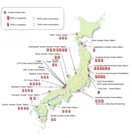
The accident at the Fukushima Dai-ichi Nuclear Power Plant (hereafter referred to as FDNPP) is extremely challenging to simulate because it was affected by a wide range of influence factors: site location, ocean proximity, uncertainty associated with numerical weather prediction and rapid evolution of weather conditions and power plant type. The FDNPP (Figure 1) is located at mid-latitudes on the East coast of Honshu, the largest island of Japan, facing directly the Pacific Ocean. This area is exposed to strong wind gusts changing direction instantaneously and fast eastbound oceanic currents [23].
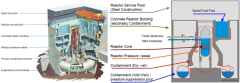
The Dai-ichi Power Plant includes six Boiling Water Reactors (BWR) designed through a joint venture by General Electrics, Toshiba and Hitachi in the 1960s (Figure 2).
The reactors are inside Mark I containment structures, consisting of a concrete building housing the Reactor Pressure Vessel (RPV) and surrounded by a Primary Containment Dry well. A toroidal pressure suppression pool is beneath the RPV and a spent fuel pool is also located inside the reactor building. A reactor service-floor seals the top of the building [24]. The BWR working parameters were monitored in the reactor control room (Figure 3).
On March 11, 2011, at 14:46 local time (05:46 UTC), a 9.0 magnitude earthquake stroke the ocean seafloor 130 km East of Sendai (Honshu island). It was a double quake of 3 minutes that shook an area 650 km long, shifting it horizontally by 10-20 m. This made Japan move several meters to the East and sank its local coastline by half a meter. At the time of the Earthquake, 11 reactors at 4 nuclear power sites were operating and all automatically shut-down according to emergency procedures. Fukushima Dai units 4, 5 and 6 were undergoing refueling and not operating at that time. Fukushima Dai units 1 (Ichi), 2 and 3 automatically shut down the fission chain reactions by inserting control rods following the “scram” rapid shut-down procedure [23]. Main power for electronics and cooling systems was lost and regained immediately as soon as the emergency diesel generators became operative. Overall, the reactors proved robust seismically, sustaining a 0.56 g acceleration. However, the massive earthquake generated a huge tsunami; forty-one minutes after the earthquake, a first wave reached the coastline, followed, 8 minutes later by a second and taller one, 12 to 15 m high [23]. The tsunami waters flooded an area of about 560 km2, damaging ports, towns and destroying over one million buildings/houses. Casualties directly related to the tsunami were 19,000. Emergency plans were activated by the Government, not expecting that another emergency was about to arise [23]. When the largest tsunami wave struck, the 10 m high FDNPP seawall was overwhelmed and seawater rapidly flooded the lower floors hosting the emergency backup diesel generators (Figure 4, [25]).
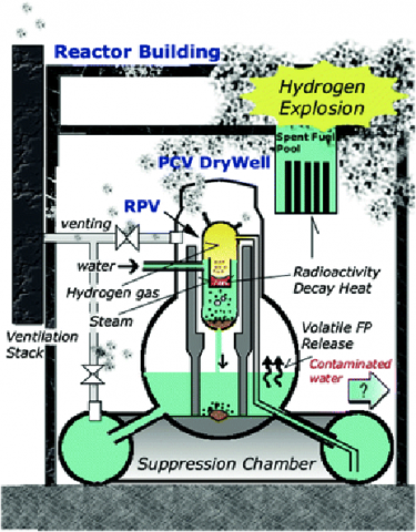
The generators serving unit 6, built uphill, and unit 5 were not flooded and kept on operating. The other generators failed, thus cutting power supply to the coolant water pumps, designed to guarantee continuous water circulation for many days in order to prevent fuel rods melting from the decay-heat of the fission products. Secondary electrical batteries kept on powering the emergency pumps, but when they ran out of charge on March 12, water circulation ceased and units 1, 2 and 3 began to overheat, leading to core meltdowns at the bottom of each RPV. In the absence of cooling, the decay heat produced steam in the RPV, increasing pressure. Then, steam relief valves opened to reduce the steam into the wet well, thus decreasing the liquid level in the RPV and increasing core degradation (Figure 5, [24]). The rising temperature led to the release of fission products from the fuel rod gaps. When 1200 °C were reached, the zircaloy cladding of the rods underwent an exothermic reaction with water, releasing free hydrogen gas. The zircaloy also reacted with uranium dioxide generating zirconium dioxide and metallic uranium. Hydrogen gas was pushed via the wet well into the dry well. Meltdown proceeded with the release of fission products: uranium/plutonium remained in the core, cesium and iodine condensed into airborne aerosols, and xenon was released in the form of dissolved atoms or intergranular or intragranular gas bubbles. As the containment urged depressurization, ventilation valves were opened and part of the hydrogen and the fission aerosols were dispersed into the atmosphere. A hydrogen leakage occurred in proximity to the wet well of unit 2, producing an explosion and uncontrolled release of gas, highly contaminated water and fission product aerosols. Hydrogen reached concentration levels leading to explosions below the reactor service floors, causing the destruction of the steel-frame rooves and the discharge of volatile and airborne fission products together with hydrogen and steam into the atmosphere. Although the worst meltdown occurred inside unit 2, casing the highest contamination of the seawater used for cooling purposes, it is estimated that reactors 1, 2 and 3 caused the highest radioactivity releases to the air [26].
Figure 1. Japan’s nuclear energy plants (https://www.oecd-nea.org/news/2011/NEWS-02.html)
Figure 2. FDNPP seen from the coastline and sketch showing the location of the reactors (https://en.wikipedia.org/wiki/Fukushima_Daiichi_nuclear_disaster)
Figure 3. Structure of a BWR in detail (http://www.archivionucleare.com/index.php/2011/03/16/reattori-bwr-incidente-nucleare-fukushima-daiichi/)
Figure 4. An aerial picture showing FDNPP flooded area [25]
Figure 5. Schematic drawing of the reactor damage and behavior of radioactive materials [24]
3.2 Radioactivity dispersal into the atmosphere
Modeling of activity dispersal in this work was based on the following considerations:
a) Most of the dispersal in the air occurred during the very first days following the tsunami, therefore, the analysis focused on March 15, 2011, which recorded the highest amount of dispersion [27];
b) The dispersion was the result of radioactive leakage, venting and hydrogen explosions occurring at different times and at different heights, from situations evolving in different reactor and containment structures [28];
c) Due to existing variables related to space (different starting locations) and time (leaks, vents and explosions at different times) together with different responses carried out at the different locations, the analysis and calculation was complex and thus aimed at a general result considered helpful for first responders to begin their operations during the emergency;
d) Heavy radionuclides remained confined in the proximity of the reactors or transported into the ocean by return waters from the flood. For aerial dispersal, two radionuclides were aerosolized and carried away inside the plume, posing the main threat: Iodine 131 and Cesium 137 (hereafter referred to as I-131 and CS-137). I-131 has a half-life of 8 days, if it enters the body, it concentrates in the thyroid (hence, it is used in metabolic radiotherapy of thyroid cancer). People are only affected in the few days after release, and the rainfall may significantly reduce atmospheric concentration of the radionuclide. Cs-137 does not target any specific organ or tissue, and its biological half-life is roughly 70 days without treatment. However, if not correctly managed, the radionuclide could cause significant exposure over a large time frame. Moreover, the effective dose received in a short time frame may still pose a threat because of the long term stochastic effects [29, 30];
e) Radioactive plumes in the atmosphere and their impact on the ground can be simulated using as input atmospheric dispersion models with two different approaches:
- using reactor physics and the knowledge of the initial state of the system (requires a lot of data and a precise knowledge of the events that occurred in the facility).
- coupling environmental measurements and atmospheric dispersion simulations to determine release rates and compare these results with experimental data. In this case, the quality of the source term depends on (1) accuracy of the weather data used as to transport and disperse radionuclides; (2) quantity/relevance of the measurements. Simplified approaches were those of the Japan Atomic Energy Agency (JAEA) [31, 32]. Since 2011, several methods have been described which couple environmental measurements and atmospheric dispersion models and generated estimates of the source term [32].
f) A final comparison with the radiation measurements in the environment is fundamental to evaluate the simulation [32].
Our HotSpot simulations were performed with data inputs from March 15, 2011, the day with the highest continuous release rate measured in the atmosphere as shown in Figure 6 [32].
We also used the emission rates of Cs-137 (becquerel per hour) from FDNPP on March 15th, 2011 (see Table 1 [32]).
3.3 Weather conditions (15 March 2011)
Two important elements were taken into account:
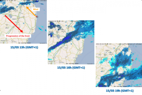
• Rainfall occurred in northern Fukushima from March 15, 2011 (9 a.m. GMT+1) to March 16, 2016 (8.00 a.m. GTM+1), as shown in Figure 7 [33].
• Wind direction and velocity influence the HotSpot algorithm. In our simulations, we used as input a southeasterly wind as shown in Figure 8 [33].
Figure 6. The total amount of I-131 and Cs-137 released in the atmosphere during the Fukushima accident between March 12 and March 16, 2011 [32, 34]
Figure 7. Progression of a rain-snow front on March 15 (GMT+1), 2011 towards the nuclear site [33]
Table 1. Emission rates (Bq/hr) from FDNPP on March 15, 2011. 1 [32]
|
Release period (local time) |
Release duration (h) |
Release 137Cs (Bq) |
Release height (m) |
|
14/3 16:00 - 14/3 17:00 |
1 |
1,3E+12 |
20 |
|
14/3 17:00 - 14/3 18:00 |
1 |
3,8E+14 |
20 |
|
14/3 18:00 - 14/3 19:00 |
1 |
3,1E+13 |
20 |
|
14/3 19:00 - 14/3 20:00 |
1 |
3,6E+13 |
20 |
|
14/3 20:00 - 14/3 23:00 |
3 |
3,9E+13 |
20 |
|
14/3 23:00 - 15/3 02:00 |
3 |
3,6E+14 |
20 |
|
15/3 02:00 - 15/3 03:00 |
1 |
1,0E+14 |
20 |
|
15/3 03:00 - 15/3 08:00 |
5 |
5,0E+13 |
20 |
|
15/3 08:00 - 15/3 10:00 |
2 |
6,6E+13 |
20 - 100 |
|
15/3 10:00 - 15/3 12:00 |
2 |
4,4E+14 |
20 - 100 |
|
15/3 12:00 - 15/3 14:00 |
2 |
1,5E+14 |
20 - 100 |
|
15/3 14:00 - 15/3 15:00 |
1 |
3,3E+14 |
20 - 100 |
|
|
|
2,1E+15 (Bq) Total release 137Cs on March 15, 2001 |
|
Figure 8. Different observations of wind direction coming from the East and turning over Fukushima to head North-West [34]
Figure 9. Radionuclides ground deposition from the FDNPP Accident [36]
The wind direction was also considered to affect rainfall and the deposition radionuclides on the ground [35], as shown in Figure 9 [36].
4.1 Description of the software, the model used and the weather conditions selected
In order to evaluate the TED, several simulations are performed using HotSpot Version 3.0.3 [37]. Health Physics software designed for short-term release durations and useful in predicting the consequences of radionuclide dispersal [38-41]. HotSpot is a hybrid of the well-established Gaussian Plume Model, widely used for initial emergency assessment or safety analysis planning. Virtual source terms are used to model the initial atmospheric distribution of source material following explosion, fire, resuspension, or user-input geometry [20].
The source term selected for our simulation was a mixture of I-131 (1,6x10¹⁶ Bq/h) and Cs-137 (1,5x10¹⁶ Bq/h) after Sugiyama et al. [42], the purpose of these simulations is to test the HotSpot Code as a tool to improve risk analysis during an emergency situation. The computational model we selected was the General Plume Model rather than the General Explosion Model which relies on better suited for dirty bombs scenarios because it is able to estimate the downwind radiological impact following the release of radioactive material resulting from a continuous or puff release [43].
Indeed, in the FDNPP accident, there were hydrogen explosions but they only caused the rupture of the rooves of the concrete reactor buildings and the release of the radionuclide aerosols. The plume development in the low atmosphere was determined by the action of the winds and the ground deposition was also influenced by the rainfall.
The concrete reactor buildings, where hydrogen explosions occurred, were at different heights and we selected an effective 20 m height for the simulations. The southeasterly wind direction was 135° with an average velocity of 4.85 m/s (data from the European Center Meteorological Weather Forecast for March 15, 15:00 hours local time). The selected Pasquill Class was F (stable) and the selected wind reference height was 10 m.
The International System of Measure units were chosen to run the simulations:
• Radiological units: sievert, gray, becquerel;
• Distance Unit: meter.
The authors have selected the Standard option instead the City terrain that usually result in lower doses than those displayed for Standard, due to the increased diffusion from the turbulence caused by larger building structures. Choosing Standard terrain produce the most conservative estimates (higher potential doses). Checking the “Input Surface Roughness” box allows the user to input the surface roughness height, Z0. When checked, the Standard option is automatically selected, and the City option disabled since the Z0 associated with typical city structures is already incorporated into the City sigma-z values.
The Federal Guidance Report 13 (with new ICRP-66 lung model and ICRP series 60/70 methodologies) was chosen to provide the Dose Conversion Coefficients. In the Wet Deposition window box, the “rainout” option was selected to account for rainfall effects on deposition (with a rainout coefficient of 1x10⁻³ L/s). The Rainout option takes into account possible rain fall during the release of radionuclides into the atmosphere, thus prompting the software to compute different concentrations at different heights due to particle diffusion.
4.2 Results and discussion
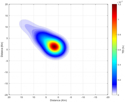
The first output of the simulation is shown in Table 2, reporting the Total Effective Dose (TED), the time-integrated respirable aerosols, the ground surface deposition, and the ground-shine dose rate at different distances and time.
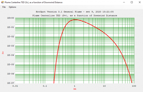
The highest values for TED and Ground Deposition are highlighted by red and blue rectangles together with the corresponding distances from the plume origin. The TED has an inverse parabolic development (Figure 10) where highest values are reached between 700 meters and 2 km (HotSpot data are reportedly accurate up to 10 km of distance).
Table 2. Table output of the HotSpot simulation for the mixture of I-131 and Cs-137 release
Figure 10. TED parabolic trend
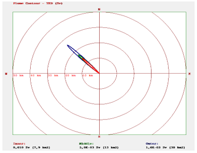
Figure 11. TED compass-centered development
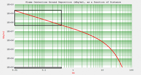
Figure 12. Ground deposition trend
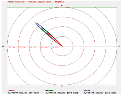
Figure 13. Ground deposition plume contour
Figure 14. TED and ground deposition from HotSpot superimposed to the aerial measured plume
The plant view of TED compass-centered development reveals the northwest direction of the plume as the wind blows from the southeast (Figure 11).
The Ground Deposition Values reported in Table 2 show an almost linearly decreasing trend because we are in a log-log diagram, with the highest values concentrated in a range of 400 m from ground zero (Figure 12). Beyond 10 km, the values cannot be considered precise anymore.
The plume contour of ground deposition in Figure 13, shows the value decreasing linearly with distance.
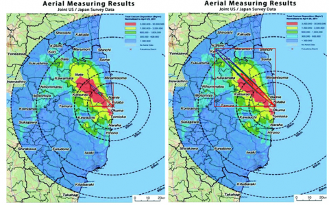
The aerial observation mission results acquired on April 29, 2011, by the U.S Department of Energy [44] were used for a comparison with the results in order to get a qualitative idea of the effectiveness of the simulation (Figure 14).
While slightly different quantities are compared (simulated “air concentration” and observed “deposition”), it can be immediately noted that the simulated plume follows the path of the measurements and the simulated amount of release also agrees with the observations.
The simulations demonstrate that HotSpot is very dependent on the source terms and the chosen environmental data. Figure 14 shows the consistency between the direction and intensity of the radioactive plume computed by HotSpot and the aerial measured event. Due to the shifting meteorological conditions, the plume measured by the US Energy Department is larger than the HotSpot simulation because it is a plume registered the 29th of April 2011, while HotSpot shows a plume after 46 minutes from the event. The advantage of HotSpot relies on its capacity to simulate a dispersion within a few minutes of work on the software, providing first responders and decision-makers with prompt and reliable data in order to take proper countermeasures to reduce risks and rescue the civilians.
HotSpot is effective for short term releases while most of the simulations and associated algorithms apply to longer periods of time and therefore result in larger contamination areas with higher concentrations. It is also designed to be more conservative and optimized for short distances providing the best accuracy within 10 km from the release source. Its use in an emergency like Fukushima would have led to an evacuation plan within 30 km from FDNPP avoiding the contaminated areas to the Northwest thus posing no hazard for radiation deterministic and stochastic effects to the population. And it would have allowed decontamination procedures to start earlier. Decision Support System (DSS) Software should always be used to take the first actions properly (do not evacuate people regardless of a radioactive plume direction). Software like HotSpot should be run not only once but many times to assess eventual changes in the environmental and/or meteorological conditions, these characteristics are very useful to produce data that can be used in to improve the risk analysis results giving a wider range of information for the safety of the first responders and the population and the security of critical infrastructures. First responders must know what’s going on and be constantly updated. The idea to apply spatial and temporal filters to the HotSpot data is useful to obtain information for larger time and geographical range in order to facilitate the planning and rescue operations during the emergencies. Other more complex software (like HPAC and other computational algorithms) should be run by the second and third wave of responders within an organization, in order to keep first responders updated on evolving scenarios. First responders and decision-makers have to ensure the continuous flow of information between responder teams, recovery and evacuation personnel of different organizations, sharing situation updates and evolving scenario analysis while rendering own personnel interoperable at different levels with other institutions/organizations working to achieve the same objectives. Such a synergetic approach to the situation should be integrated into a larger crisis management-system, where the information would be processed and tailored to the needs of the final user for the best results. It can be concluded that HotSpot, coupled with Spatio-temporal filters, can be considered a valid tool to reduce risk in case of a nuclear accident like the one in Fukushima. As a future development of this work, the authors have the intention to improve the filters and test a methodology that takes into account the role played by the orography when using expeditious software like HotSpot.
The authors plan to apply spatial and temporal filters using a suitable software (such as Matlab) to the data provided by HotSpot in order to stress it giving TED plume over a larger territory and longest time range.
The main idea behind the whole approach is to be able to increase the effectiveness of the simulations (in terms of the response to a CBRNe emergency) performed through Hotspot by applying image analysis techniques to the output plumes. This process involves the application of spatial 2D filters to the images generated by HotSpot in order to approximate the diffusive phenomena of the plumes having only 3 different discrete profile values of TED or Ground Deposition. Moreover, given the limited timespan (max 46 minutes) and limited space-temporal information of the simulations (the 2D TED or Ground Deposition distributions are only available at 46 minutes), a possible approach to estimate the space-temporal evolution of the plume may be to treat the output of the software as a linear space invariant optical-imaging system. Under such circumstances, it may be possible to understand if it is feasible to approximate the evolution of the diffusion by only applying common image-filtering techniques.
Since Hotspot only outputs a discrete plume divided in 3 threat areas (red, yellow, green) which have a single value of associated TED or Ground Deposition, a spatial varying filter (heat kernel) has been convoluted over the plume as an example to approximate a process of homogeneous and isotropic diffusion assuming a constant diffusion coefficient. This has been done to investigate the potential time evolution of a mass-density under diffusion forces. In fact, if the mass-density at t = 0 is concentrated in one single spot, then the mass-distribution at the generic time t will be given by a gaussian function whose height peak parameter is linearly related with the inverse value of the square root of t, and its variance is linearly related with t.
The plume used to test the simple spatial filter was the one presented in this paper, where the authors used a Gaussian low pass filter with sigma equal to 2 km. In such case, sigma is the parameter linearly related to the square root value of the product between the diffusion coefficient and time. Since the diffusion coefficient is not supposed to be known, sigma values (expressed in km) have been arbitrary chosen as increasing values over time. The results are shown in Figure 15.
Figure 15. TED plume with Gaussian low pass filter with sigma equal to 2 km
The application of spatial and temporal filters to HotSpot simulations may allow first responders and decision-makers to gain more information which could provide useful to plan the response operations. Although this new approach doesn’t guarantee the same precision obtained with software like COMSOL Multiphysics, it still provides time and spatial range data within a very short time span.
[1] Malizia, A., 2013/2014 CBRNe Masters Group. (2016). Disaster management in case of CBRNe events: An innovative methodology to improve the safety knowledge of advisors and first responders. Defense & Security Analysis, 32(1): 79-90. https://doi.org/10.1080/14751798.2015.1130319
[2] Jenvald, J., Morin, M., Kincaid, J.P. (2001). A framework for web-based dissemination of models and lessons learned from emergency-response exercises and operations. International Journal of Emergency Management, 1(1): 82-94. https://doi.org/10.1504/IJEM.2001.000512
[3] Andersson, K.G., Mikkelsen, T., Astrup, P., Thykier-Nielsen, S., Jacobsen, L.H., Schou-Jensen, L. (2008). Estimation of health hazards resulting from a radiological terrorist attack in a city. Radiation Protection Dosimetry, 131(3): 297-307. https://doi.org/10.1093/rpd/ncn173
[4] Werner, C.J. (2017). MCNP Users Manual-Code Version 6.2. Los Alamos National Laboratory, LA-UR-17-29981. http://permalink.lanl.gov/object/view?what=info:lanl-repo/lareport/LA-UR-17-29981.
[5] Aiginger, H., Andersen, V., Ballarini, F., Battistoni, G., Campanella, M., Carboni, M. (2005). The FLUKA code: new developments and application to 1 GeV/n iron beams. Advances in Space Research, 35(2): 214-222. https://doi.org/10.1016/j.asr.2005.01.090
[6] Agostinelli, S. (2003). GEANT4-a simulation tool kit. Nuclear Instruments and Methods in Physics Research, A506(3): 250-303. https://doi.org/10.1016/S0168-9002(03)01368-8
[7] Kawrakow, I., Rogers, D.W.O. (2019). The EGSnrc code system: Monte carlo simulation of electron and photon transport. Ionizing Radiation Standards, National Research Council Canada, Ottawa, Canada, NRCC Report PIRS-701.
[8] Salvat, F., Fernández-Varea, J.M., Sempau, J. (2006). PENELOPE-2006: A code system for Monte Carlo simulation of electron and photon transport. In Workshop Proceedings, 4(6222): 7.
[9] Leppänen, J. (2013). Serpent–a continuous-energy Monte Carlo reactor physics burnup calculation code. VTT Technical Research Centre of Finland, 4. https://www.polymtl.ca/merlin/Serpent_Dragon/Serpent_manual_2013.pdf.
[10] Wu, Y., Song, J., Zheng, H., Sun, G., Hao, L., Long, P. (2015). CAD-based Monte Carlo program for integrated simulation of nuclear system SuperMC. Annals of Nuclear Energy, 82: 161-168. https://doi.org/10.1016/j.anucene.2014.08.058
[11] Studenski, M.T., Haverland, N.P., Kearfott, K.J. (2007). Simulation, design, and construction of a 137Cs irradiation facility. Health Physics, 92(5): S78-S86. https://doi.org/10.1097/01.HP.0000253943.69777.a9
[12] Dymitrowska, M., Bourgeois, M., Mathieu, G. (2007). High performance fvfe multidomain numerical method to perform radionuclides transport calculations. Joint International Topical Meeting on Mathematics and Computations and Supercomputing in Nuclear Applications, M and C + SNA 2007, Monterey, CA; United States; 15 April 2007 through 19 April 2007; Code 70680, ISBN: 0894480596;978-089448059.
[13] Ciparisse, J., Cenciarelli, O., Mancinelli, S., Ludovici, G. M., Malizia, A., Carestia, M. (2016). A computational fluid dynamics simulation of anthrax diffusion in a subway station. International Journal of Mathematical Models and Methods in Applied Sciences, 10: 286-291.
[14] Raskob, W., Trybushnyi, D., Ievdin, I., Zheleznyak, M. (2011). JRODOS: Platform for improved long term countermeasures modelling and management. Radioprotection, 46(6): S731-S736. https://doi.org/10.1051/radiopro/20116865s
[15] Hoe, S., McGinnity, P., Charnock, T., Gering, F., Jacobsen, L.S., Sørensen, J. H. (2009). ARGOS decision support system for emergency management. In Proceedings of the 12th International Congress of the International Radiation Protection Association. Buenos Aires, Argentina: IRPA.
[16] Otrisal P. (2012). Selected software tools used for CBRN situation assessment within CZECH armed forces chemical corps. Journal of Defense Management.
[17] Auxier, J.P., Auxier II, J.D., Hall, H.L. (2017). Review of current nuclear fallout codes. Journal of Environmental Radioactivity, 171: 246-252. https://doi.org/10.1016/j.jenvrad.2017.02.010
[18] Hill, A. (2003). Using the Hazard Prediction and Assessment Capability (HPAC) hazard assessment program for radiological scenarios relevant to the Australian Defence Force. Defence science and technology organisation victoria (australia) platform sciences lab.
[19] Carestia, M., Malizia, A., Barlascini, O., Fiorini, E., Soave, P. M., Latini, G. (2016). Use of the "hotspot" code for safety and security analysis in nuclear power plants: a case study. Environmental Engineering & Management Journal (EEMJ), 15(4): 905-912. https://doi.org/10.30638/eemj.2016.098
[20] Biancotto, S., Malizia, A., Pinto, M., Contessa, G.M., Coniglio, A., D'Arienzo, M. (2020). Analysis of a dirty bomb attack in a large metropolitan area: Simulate the dispersion of radioactive materials. Journal of Instrumentation, 15(2): P02019. https://doi.org/10.1088/1748-0221/15/02/P02019
[21] Anvari, A., Safarzadeh, L. (2012). Assessment of the total effective dose equivalent for accidental release from the Tehran Research Reactor. Annals of Nuclear Energy, 50, 251-255. http://dx.doi.org/10.1016/j.anucene.2012.07.002
[22] Cacciotti, I., Aspetti, P.C., Cenciarelli, O., Carestia, M., Di Giovanni, D., Malizia, A. (2014). Simulation of Caesium-137 (137CS) local diffusion as a consequence of the Chernobyl accident using HOTSPOT. Defence S&T Technical Bulletin, 7(1): 18-26. https://doi.org/10.1021/om034263o
[23] Baba, M. (2013). Fukushima accident: what happened? Radiation Measurements, 55: 17-21. https://doi.org/10.1016/j.radmeas.2013.01.013
[24] Takada, M., Suzuki, T. (2013). Early in situ measurement of radioactive fallout in Fukushima city due to Fukushima Daiichi nuclear accident. Radiation Protection Dosimetry, 155(2): 181-196. https://doi.org/10.1093/rpd/ncs320
[25] Narabayashi, T. (2013, July). Countermeasures derived from the lessons of the fukushima daiichi nuclear power plant accident. In International Conference on Nuclear Engineering, 55812: V004T09A122. https://doi.org/10.1115/ICONE21-16895
[26] Hachiya, M., Akashi, M. (2016). Lessons learned from the accident at the Fukushima Dai-ichi Nuclear Power Plant—more than basic knowledge: Education and its effects improve the preparedness and response to radiation emergency. Radiation Protection Dosimetry, 171(1): 27-31. https://doi.org/10.1093/rpd/ncw182
[27] Thakur, P., Ballard, S., Nelson, R. (2013). An overview of Fukushima radionuclides measured in the northern hemisphere. Science of the Total Environment, 458: 577-613. https://doi.org/10.1016/j.scitotenv.2013.03.105
[28] Mizokami, S., Kumagai, Y. (2015). Event sequence of the Fukushima Daiichi accident. In Reflections on the Fukushima Daiichi Nuclear Accident, pp. 21-50. https://doi.org/10.1007/978-3-319-12090-4_2
[29] Hirao, S., Yamazawa, H., Nagae, T. (2013). Estimation of release rate of iodine-131 and cesium-137 from the Fukushima Daiichi nuclear power plant: Fukushima NPP accident related. Journal of Nuclear Science and Technology, 50(2): 139-147. https://doi.org/10.1080/00223131.2013.757454
[30] Long, P.K., Hien, P.D., Quang, N.H. (2019). Atmospheric transport of 131I and 137Cs from Fukushima by the East Asian northeast monsoon. Journal of Environmental Radioactivity, 197: 74-80. https://doi.org/10.1016/j.jenvrad.2018.12.003
[31] Chino, M., Nakayama, H., Nagai, H., Terada, H., Katata, G., Yamazawa, H. (2011). Preliminary estimation of release amounts of 131I and 137Cs accidentally discharged from the Fukushima Daiichi nuclear power plant into the atmosphere. Journal of Nuclear Science and Technology, 48(7): 1129-1134. https://doi.org/10.1080/18811248.2011.9711799
[32] Katata, G., Chino, M., Kobayashi, T., Terada, H., Ota, M., Nagai, H. (2015). Detailed source term estimation of the atmospheric release for the Fukushima Daiichi Nuclear Power Station accident by coupling simulations of an atmospheric dispersion model with an improved deposition scheme and oceanic dispersion model. Atmospheric Chemistry and Physics, 15(2): 1029-1070. https://doi.org/10.5194/acp-15-1029-2015
[33] Isnard, O., Raimond, E., Corbin, D., Denis, J. (2012). Radioactive source term and release in the environment. Eurosafe, IAEA Report, 43: 162-194.
[34] Terada, H., Katata, G., Chino, M., Nagai, H. (2012). Atmospheric discharge and dispersion of radionuclides during the Fukushima Dai-ichi Nuclear Power Plant accident. Part II: verification of the source term and analysis of regional-scale atmospheric dispersion. Journal of Environmental Radioactivity, 112: 141-154. https://doi.org/10.1016/j.jenvrad.2012.05.023
[35] Saito, K., Ogawa, S. (2016). Radioactive pollution estimate for Fukushima nuclear power plant by a particle model. International Archives of the Photogrammetry, Remote Sensing and Spatial Information Sciences, XLI-B8: 163-168. https://doi.org/10.5194/isprs-archives-XLI-B8-163-2016
[36] Mikami, S., Maeyama, T., Hoshide, Y., Sakamoto, R., Sato, S., Okuda, N. (2015). Spatial distributions of radionuclides deposited onto ground soil around the Fukushima Dai-ichi Nuclear Power Plant and their temporal change until December 2012. Journal of Environmental Radioactivity, 139: 320-343. https://doi.org/10.1016/j.jenvrad.2014.09.010
[37] Homann, S.G., Aluzzi, F. (2013). HotSpot health physics codes version 3.0 user’s guide. Lawrence Livermore National Laboratory, CA, USA.
[38] Dombroski, M.J., Fischbeck, P.S. (2006). An integrated physical dispersion and behavioral response model for risk assessment of radiological dispersion device (RDD) events. Risk Analysis: An International Journal, 26(2): 501-514. https://doi.org/10.1111/j.1539-6924.2006.00742.x
[39] Sohier, A., Hardeman, F. (2006). Radiological Dispersion Devices: Are we prepared? Journal of Environmental Radioactivity, 85(2-3): 171-181. https://doi.org/10.1016/j.jenvrad.2004.04.017
[40] Rother, F.C., Rebello, W.F., Healy, M.J., Silva, M.M., Cabral, P.A., Vital, H.C., Andrade, E.R. (2016). Radiological risk assessment by convergence methodology model in RDD scenarios. Risk Analysis, 36(11): 2039-2046. https://doi.org/10.1111/risa.12557
[41] Yoo, H., Lee, J.H., Kwak, S.W. (2011). Analysis of radiological terrorism on metropolitan area. Energy and Environment Research, 1(1): 24. https://doi.org/https://doi.org/10.5539/eer.v1n1p24
[42] Sugiyama, G., Nasstrom, J., Pobanz, B., Foster, K., Simpson, M., Vogt, P. (2012). Atmospheric dispersion modeling: Challenges of the Fukushima Daiichi response. Health Physics, 102(5): 493-508. https://doi.org/10.1097/HP.0b013e31824c7bc9
[43] Homann, S.G, Aluzzi, F. (2014). HotSpot Health Physics Codes Version 3.0 User’s Guide. LLNL-SM-636474. https://narac.llnl.gov/content/assets/docs/HotSpot- UserGuide-3-0.pdf.
[44] Results of Airborne Monitoring by the Ministry of Education, Culture, Sports, Science and Technology and the U.S. Department of Energy (2011). https://radioactivity.nsr.go.jp/en/contents/4000/3180/24/1304797_0506.pdf.