
Rasha A. Mohammed | Mohammed Obaid Mustafa*
© 2026 The authors. This article is published by IIETA and is licensed under the CC BY 4.0 license (http://creativecommons.org/licenses/by/4.0/).
OPEN ACCESS
The primary objective of this study is to conduct a comparative evaluation of traditional Volt-VAR control strategies and adaptive gain-scheduled strategies. Modern distribution networks face significant challenges regarding voltage stability, especially under stressed loading conditions. In this study, the IEEE 33-bus system was utilized as a benchmark. Both traditional and adaptive control strategies using MATLAB and MATPOWER software have been used in this work. The proposed adaptive approach utilizes a gain-scheduled control mechanism supervised by a stability-margin index, allowing the controller to adjust its parameters dynamically based on the system’s operating state. The simulation results demonstrate that the adaptive controller significantly outperforms the traditional fixed-parameter approach. Key findings include an increase in the minimum system voltage from 0.9038 p.u. to 0.9491 p.u., reduction in the number of weak buses from 21 to only 3, an enhancement of the stability margin to 1.0981, and the reactive power losses showed a slight increase. Finally, the adaptive gain-scheduled control is also considered a more robust solution than the existing method.
voltage stability, Volt-VAR control, adaptive control, load flow, IEEE 33-bus system, V-Q modal analysis, MAT
The growth of renewable energy sources (RESs) like photovoltaics (PV) or wind systems has led to the revolutionization of the current grid [1]. These new resources increase sustainability but create issues like intermittency of supply, poor ability to provide reactive power, bidirectional power flow, and voltage control, leading to a voltage instability problem, especially in systems with a higher ratio of resistance to reactance (R/X) [2]. Voltage stability has become an important challenge to overcome in the operation of these new energy supplies. The lack of proper reactive power supply under stressful network loading can cause voltage problems or even voltage collapse, and therefore it is crucial to ensure adequate voltages at all times. Some of the analytical techniques used for this task include load-flow, V-Q modal analysis, and continuation power flow (CPF) methods. [3]. Compensation of reactive power using Volt-VAR control has shown great promise as an approach to voltage control. However, traditional Volt-VAR control depends on fixed gains and system properties, limiting performance under different operating conditions [4]. An alternative approach that can improve such performance limitations is the use of adaptive control, which allows gains to be changed dynamically depending on system conditions [5]. In this regard, an adaptive gain-scheduling Volt-VAR controller with supervisory stability margin modulation is proposed as a framework to enhance the performance of reactive power compensation. Local adaptive gain-scheduling control with supervisory control using voltage stability margin improves both reactive power support and the robustness of the system under stress [6]. IEEE 33-bus radial distribution system is used as a test case because of its poor voltage quality properties. The work involves analysis to identify weak buses based on V-Q modal analysis and system stability assessment using CPF, in addition to a comparison between traditional and adaptive controllers. It further investigates the benefits of increasing control buses and raising reactive power limits to show that distributed control of multiple buses outperforms high reactive power levels [7].
Ren et al. [8] proposed an extremum-seeking adaptive droop-based Volt-VAR control strategy for model-free voltage regulation. The method improves voltage support and reduces power losses using local measurements, outperforming conventional droop control with adaptability under varying operating conditions. Arnold et al. [9] proposed decentralized, model-free adaptive control of inverter-based distributed energy resources and validated it on IEEE 37- and 8500-node test feeders. Its main strength is communication-free adaptation that mitigates adverse interactions among inverter controls. Unlike that framework, the present study keeps the same Volt-VAR characteristic for both cases and isolates the effect of bounded gain-scheduling with stability-margin supervision. Cheng et al. [10] developed a communication-free self-adaptive local voltage controller that updates droop slope and intercept from local voltage measurements, with analytical stability and convergence properties. In contrast, the present method keeps the Volt-VAR breakpoints fixed and adapts only a bounded multiplicative gain, supplemented by stability-margin supervision. Lumina et al. [11] presented a PV controller design based on an adaptive Volt-VAR algorithm for voltage stability in power systems. The proposed controller monitored voltage variations and dynamically regulated reactive power injection through inverter-based Volt-VAR control to maintain system voltage within acceptable stability limits. The adaptive scheme was successful in enhancing voltage recovery, reducing losses, and improving voltage stability in dynamic environments. From simulations, the adaptive Volt-VAR controller was able to raise bus voltages from critically low levels to stable operating ranges. This indicated better performance compared to traditional voltage regulation schemes. Murzakhanov et al. [12] optimized inverter Volt-VAR rules subject to nonlinear dynamic-stability conditions and demonstrated the design on an IEEE 141-bus feeder. The method provides stability-aware rule design but requires a feeder model and an offline optimization stage; the present method instead preserves the conventional Volt-VAR curve and adds bounded gain-scheduling with stability-margin supervision. Doni et al. [13] analyzed voltage stability in radial power networks through shunt capacitor placement for reactive power compensation. The technique, employed on IEEE 33 and 69-bus systems, managed to raise the minimal voltage level from 0.9131 p.u. to 0.95 p.u. while decreasing power losses by approximately 22%. Although the procedure is effective, it is not adaptive in different operating conditions. Notwithstanding these developments, very little research effort has been made into incorporating adaptive gain-scheduling in supervisory stability margin controls and multi-bus coordination.
The following is an outline of the contributions made by this research work:
-A comparison between traditional and adaptive gain-scheduled Volt-VAR controllers is conducted in stressed conditions.
-Two-layer control is introduced by integrating adaptive gain-scheduling and supervisory stability margin modulation control.
-Reactive power control at distributed multiple buses is utilized for better voltage regulation than single bus compensation.
-The impact of the number of control buses and the limit on reactive power is considered to achieve better voltage control across the entire network.
-The introduced adaptive control outperforms the traditional controller by minimizing weak buses by 50% and increasing stability margin and minimum voltage.
4.1 System description
This section presents the test system, operating scenarios, and simulation framework used for voltage stability assessment and controller comparison. The analysis is carried out in MATLAB/MATPOWER using the IEEE 33-bus radial distribution system as a benchmark network. The IEEE 33-bus system is widely adopted in studies of voltage regulation, loss minimization, and reactive power compensation. It consists of 33 buses and 32 radial branches. Since the network is radial and has an R/X ratio that is high, it makes it very sensitive to changes in load conditions and reactive power shortage, thus making it ideal for voltage stability analysis [14]. The system is analyzed under stressed operating conditions in order to detect voltage weaknesses and to assess the efficiency of reactive power injection.
4.2 Selection of control buses and statement of problem
Buses for control are chosen depending on voltage weaknesses, modal participation analysis and dynamic changes of weak bus locations in case of reactive power compensation. For implementation purposes, multi-bus reactive power support is used at buses 18,33,32,16,30 [15].
The problem being tackled in this paper is improving voltage stability by providing more reactive support under stressed operating conditions and voltage violation minimization. This was achieved through comparison between Volt-VAR controller and an adaptive gain-scheduled controller.
4.3 Base-case and stressed-case formulation
Two scenarios are defined as the base-case and stressed-case. The base-case describes the initial loading scenario of the IEEE 33-bus test system that would be used to compute the initial voltage profile. Voltage profiling is done using load flow analysis to identify important metrics such as minimum voltage (Vmin), active and reactive power losses (Ploss, Qloss), and the total number of buses below 0.95 per unit. The stressed case describes the loading scenario designed to simulate the proximity of the system to voltage instability. This is achieved by loading the system up to a point where the loading factor is 1.10, plus an extra factor of 1.03 on downstream buses. This strategy is chosen based on the greater vulnerability of distant buses to voltage fluctuations in radial networks. The stressed system is then analyzed through load flow analysis.
This model is essential in ensuring a uniform standard of evaluation of controller performance since both the conventional and adaptive controllers are subjected to similar stresses[16].
4.4 Software programs used in this study
Program 1: Load-flow analysis
Power flow analysis is conducted through the use of Newton Raphson (NR) method through MATPOWER. The equations solved by the method are those representing power balance at each node:
Pi = Vi ∑j=1nVj (Gij cos θij + Bij sin θij) (1)
Qi = Vi ∑j=1nVj (Gij sin θij − Bij cos θij) (2)
NR method is chosen as it is more numerically stable and provides the Jacobian matrix necessary for voltage stability studies. While forward-backward sweep is normally used for radial systems, NR provides consistency regardless of operation mode and further facilitates V-Q modal analysis.
NR Method relies on an iterative solution based on Jacobian representation [17]:
[ΔP] = [J1 J2][Δθ] (3)
[ΔQ] = [J3 J4][ΔV] (4)
Load flow analysis results form the starting point in the diagnosis procedure where the voltage instability is detected, and the weakest bus is determined according to the minimum voltage criterion:
Vmin = min(Vi) (5)
Program 2: V-Q modal analysis
V-Q modal analysis is used in detecting weak buses by applying voltage stability considerations rather than mere voltage levels. It makes use of the reduced Jacobian matrix, which represents how variations in reactive power influence voltage levels:
ΔQ = JRΔV (6)
The reduced Jacobian is derived from the NR Jacobian:
JR = J4 − J3J1−1J2 (7)
Voltage stability is assessed through eigenvalue analysis:
JRΦi = λiΦi (8)
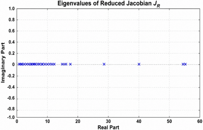
A small value of λmin indicates weak voltage stability. In this study, the obtained value λₘᵢₙ = 0.0215 confirms that the system operates under stressed conditions.
To identify the most critical bus, participation factors are used:
Pki = Φkiψik (9)
The weak bus is determined as the one with the highest participation factor in the critical mode. The analysis identifies Bus 18 as the most critical bus, which is consistent with load-flow results.
Program 3: Continuation power flow
CPF is used to evaluate the voltage stability margin and determine the voltage collapse point by tracing system behavior under increasing load. The loading model is expressed as:
PD(λ) = PD0(1 + λ) (10)
QD(λ) = QD0(1 + λ) (11)
The maximum loading factor (λmax) is the upper limit of the system's loadability, whereas the voltage at the nose of the collapse curve is referred to as Vnose.
The CPF method generates important features such as the P-V curve of the weak bus, the minimum voltage as a function of the loading factor, and the active power loss as a function of loading.
The outputs of CPF are complementary to the load flow analysis and the V-Q modal analysis because they provide a measure of the system's stability margin, whereas the latter determine the voltage violation points.
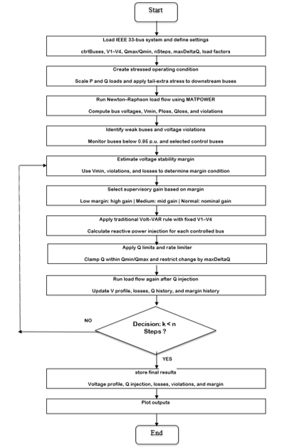
Program 4: Traditional Volt-VAR controller
The classic Volt-VAR control system operates on the basis of a predefined piecewise linear function of bus voltage and reactive power output. Reactive support is offered when bus voltage is low while reactive power absorption takes place when bus voltage is high [18]:
Q = f(V) (12)
To ensure practical operation, the control signal is constrained within reactive power limits:
Qmin ≤ Q ≤ Qmax (13)
and a rate limiter is applied to prevent abrupt changes:
ΔQ(k) = Q(k) − Q(k − 1), |ΔQ(k)| ≤ ΔQmax (14)
The traditional controller is used as a baseline for comparison, and its performance is evaluated in terms of voltage profile, reactive power support, and stability margin.
The procedures of the traditional method is given in Figure 1.
Figure 1. Flowchart of the traditional Volt-VAR controller with supervisory stability-margin mechanism
Program 5: Adaptive gain-scheduled Volt-VAR controller
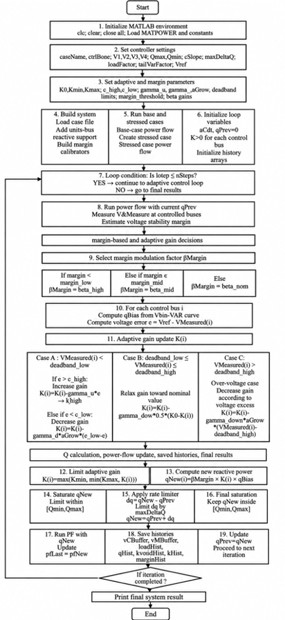
The proposed controller preserves the conventional Volt–VAR structure while incorporating two adaptive layers: (i) local gain-scheduling based on voltage error, and (ii) supervisory modulation based on the estimated voltage stability margin. Multi-bus reactive support is applied at selected control buses.
The adaptive control law is defined as:
e(k) = Vref − V(k) (15)
Qadp(k) = K(k)Qvv(k) (16)
Qraw(k) = βmargin(k)K(k)Qvv(k) (17)
where, K(k) is the bounded local adaptive gain and βmargin(k) is the supervisory stability-margin factor [19]. The implemented values are K0 = 1.00, Kmin = 0.80, Kmax = 2.00, ehigh = 0.05, elow = 0.015, γup = 0.35, and γdown = 0.08, with a voltage deadband of 0.99–1.01 p.u.
For V(k) < 0.99 p.u., the gain increases by γup[e(k) − ehigh] when e(k) > ehigh and decreases by γdown[elow − e(k)] when e(k) < elow. Inside 0.99–1.01 p.u., K is relaxed toward K0; above 1.01 p.u., it is reduced in proportion to the voltage excess.
The supervisory factor is βmargin = 1.35 for M(k) < 0.08, 1.15 for 0.08 ≤ M(k) < 0.18, and 1.00 otherwise. After each update, K is clipped to [Kmin, Kmax]. The final reactive-power command is saturated and rate-limited:
Qmin ≤ Q ≤ Qmax, |ΔQ(k)| ≤ ΔQmax (18)
Gain clipping, reactive-power saturation, the ΔQmax = 0.05 MVAr/step rate limit, and deadband-based relaxation prevent unbounded gain growth and abrupt iteration-to-iteration changes while retaining stronger support under undervoltage.
4.5 Expansion of control-buses and reactive power limits
In the present study, both control-buses and reactive power limits are considered as desisgn variables, which play a vital role in improving the voltage stability. The control-buses have been expanded to a multi-control bus system: 18,33,32,16,30.
This expansion has been done on account of relocation of weak bus location after reactive compensation, which indicates that the voltage instability has been shifted to another bus [20].
4.6 Objective function and performance indices
The objective function of this research work is to maximize voltage stability by improving voltage profile, reducing losses and minimizing stability margin. The above objectives can be represented mathematically in form of multi-objective function as follows, min [ N (V < 0.95), Ploss, Qloss], max [Vmin, M(k)]. Performance evaluation is based upon normalized improvement indices for voltage stability, losses, and weak bus as follows:
Voltage Improvement (%) = (Vnew − Vbase) / Vbase × 100% (19)
Loss Reduction (%) = (Pbase − Pnew) / Pbase × 100% (20)
Weak Bus Reduction (%) = (Nbefore − Nafter) / Nbefore × 100% (21)
4.7 General computational approach
The general computational approach is described below:
IEEE 33-bus test system is loaded using MATPOWER.
Base-case load flow is performed.
Stressed case is generated by use of load and tail extra factors.
Stressed-case load flow is carried out.
Weak buses are determined by using the voltage profile.
Perform V-Q modal analysis using reduced Jacobian, eigenvalues, and participation factors.
Perform CPF analysis to derive P-V curve, margin of loading, and the nose point.
Determine initial and expanded control-bus set.
The Traditional Volt-VAR controller is used.
Application of the adaptive gain-scheduled Volt-VAR controller with stability-margin modulation.
Voltages, losses, weak buses, reactive power injection, gain evolution, and stability margin are recorded.
Compare the performance of the controllers using the selected indices.
All controllers will be analyzed under the same network configuration, stressed operating conditions, control buses, reactive limits, and performance indices.
The procedures of the adaptive method are given in Figure 2.
Figure 2. Flowchart of the adaptive gain-scheduled Volt-VAR controller
The results are organized from the uncontrolled benchmark to the controller comparison and robustness evaluation.
5.1 Base-case load flow
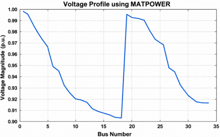
Figure 3 shows the voltage profile for the IEEE 33-bus distribution network under base-case loading, where the graph represents the relationship between bus number and bus voltage (p.u).
Figure 3. Voltage profile of the IEEE 33-bus system under base-case condition
The result of IEEE 33-bus system (MATPOWER) are listed in Table 1.
Table 1. Load flow results of IEEE 33-bus system (MATPOWER)
|
Parameter |
Value |
|
Power flow status |
Converged successfully |
|
Minimum voltage bus |
18 |
|
Minimum voltage (p.u.) |
0.903781 |
|
Total real power loss (MW) |
0.210981 |
|
Total reactive power loss (MVAr) |
0.143124 |
|
Buses below 0.95 p.u. |
21 |
From the table and figure above, it can be observed that Bus 18 is the most vulnerable bus with minimum voltage equal to 0.9038 p.u. This suggests that there is severe voltage instability, and hence, the reason for the selection of this bus for subsequent analysis and control design. Also, 21 buses have voltages lower than 0.95 p.u., suggesting the prevalence of under-voltage conditions rather than isolated cases. Moreover, the active power losses in the network amount to 0.21098 MW, pointing towards inefficiency. All these outcomes suggest that the base case system functions close to undesirable voltage levels and needs reactive power compensation.
5.2 Identification of weak buses based on V-Q modal analysis
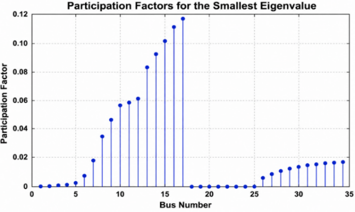
Figure 4 displays the participation factor distribution corresponding to the lowest eigenvalue of the reduced Jacobian matrix, linking bus numbers and participation factors.
Figure 4. Participation factor distribution with respect to bus number for the smallest eigenvalue
Figure 5. Eigenvalue distribution of the reduced Jacobian JR in the complex plane
Figure 5 displays the eigenvalue map of the reduced Jacobian matrix JR shown in the figure above demonstrates the correlation between the real and imaginary parts of the eigenvalues. Voltage stability can be analyzed based on this eigenvalue map where the most critical voltage stability eigenvalue is the lowest among all those close to the origin.
The results of V-Q Modal analysis results of IEEE 33-bus system (MATPOWER) are listed in Table 2. From the table, it is clear that the V-Q Modal Analysis produced an extremely low minimum eigenvalue of λmin = 0.0215, which implies poor voltage stability and that the system is operating near its stability limit when loaded heavily. The participation factor analysis shows that Bus 18 is the most important bus with a high participation factor value of 0.1182, then Bus 17 and Bus 16. This means that Bus 18 is the optimal place to install controllers for reactive power compensation. From the clustering of high participation factors, it is evident that the voltage weakness is confined to a specific region and not any bus.
Table 2. V-Q modal analysis results of IEEE 33-bus system (MATPOWER)
|
Parameter |
Value |
|
Smallest eigenvalue of JR |
0.02149597 |
|
Weakest mode index |
1 |
|
Weakest bus (participation factor) |
18 |
|
Top weak buses |
Based on highest participation factors corresponding to smallest eigenvalue |
5.3 Voltage stability assessment through continuation power flow
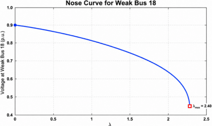
Figure 6 presents the graph of P-V nose curve that has been derived using CPF for Weak Bus 18, which shows loading factor (λ) versus bus voltage magnitude (p.u.).
Figure 6. Relationship between voltage magnitude and loading factor (λ) for weak Bus 18 using continuation power flow (CPF)
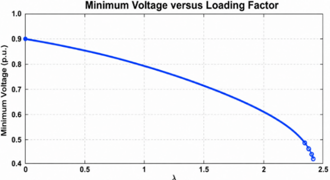
As the loading factor increases, the voltage initially falls slowly and then abruptly at the critical point, resulting in the classic nose curve associated with voltage collapse. The maximum loading margin is about λmax ≈ 2.4. This denotes the maximum loadability limit beyond which the system becomes unstable. Figure 7 shows the loading factor λ versus the minimum system voltage, demonstrating the behavior of the minimum bus voltage as system loading varies.
Figure 7. Effect of loading factor λ on minimum system voltage
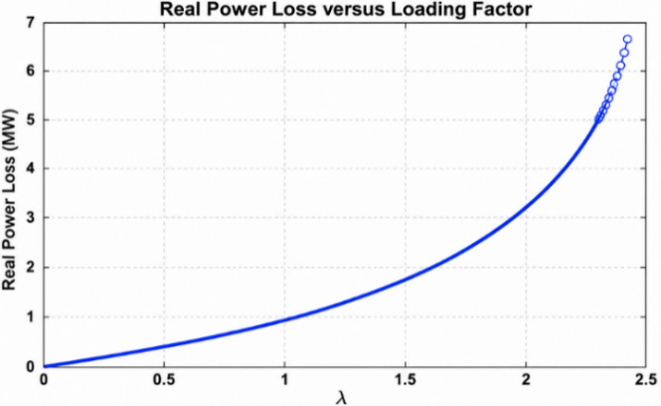
The voltage at the nose point is about: Vnose = 0.42 pu. Figure 8 below depicts the correlation between loading factor λ and real power losses, indicating the changes in active power losses with increasing loading.
Figure 8. Dependence of real power loss on the loading factor λ
According to the above figure, the value of real power loss near the limit of instability is Ploss ≈ 6.3 MW.
5.4 Traditional Volt-VAR controller performance with a margin supervision scheme
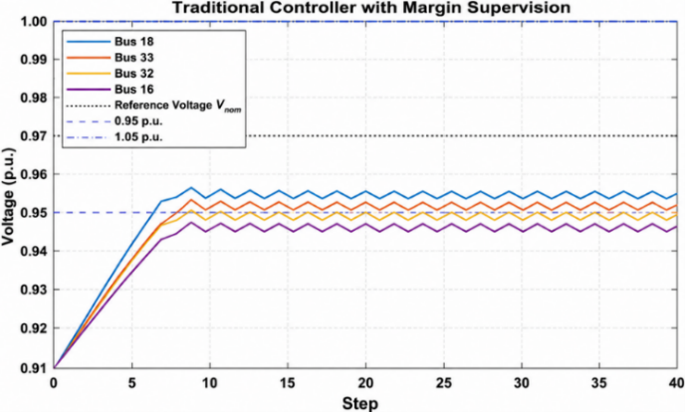
Figure 9 shows the iteration-wise voltage evolution of the controlled buses and system minimum voltage under traditional Volt-VAR control.
Figure 9. Voltage control of regulated buses using conventional Volt-VAR control method
The controller raises the minimum voltage from the stressed value of 0.9022 per unit to 0.9481 per unit, moving the network close to the 0.95-per-unit operating threshold. Figure 10 shows the corresponding reactive-power injection across the controlled buses.
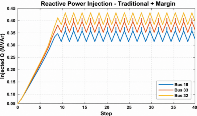
Figure 10. Reactive power injection behavior of controlled buses through traditional Volt-VAR control
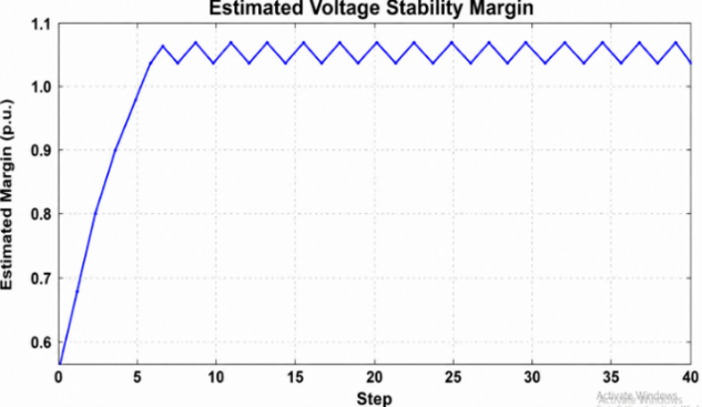
The reactive-power commands settle into bounded oscillatory adjustments within the imposed limits, reflecting the combined effect of the fixed Volt-VAR curve, supervisory factor, and rate limiter. Figure 11 shows the iteration-wise evolution of the estimated stability margin under traditional control.
Figure 11. Dynamic behavior of the estimated voltage stability margin using the traditional control approach
Table 3. Comparative analysis between base, stressed, and controlled cases (IEEE 33-bus power system)
|
Parameter |
Base Case |
Stressed Case |
Controlled Case |
|
Vmin (p.u.) |
0.9131 |
0.9022 |
0.9481 |
|
Min Bus |
18 |
18 |
13 |
|
Buses < 0.95 |
21 |
21 |
6 |
|
Ploss (MW) |
0.2027 |
0.2594 |
0.1868 |
|
Qloss (MVAr) |
0.1351 |
0.1730 |
0.1278 |
|
Margin |
— |
— |
1.0847 |
The estimated margin rises rapidly during the initial control steps and then remains in a bounded operating range, indicating improved robustness according to the margin estimator used in this study. Traditional control provides substantial baseline improvement, but its local Volt-VAR characteristic does not adapt its gain to the measured voltage error. This motivates the adaptive comparison in Section 5.5. Table 3 summarizes the base, stressed, and traditional-controlled cases. Relative to the stressed case, the traditional controller increases Vmin from 0.9022 to 0.9481 p.u., reduces buses below 0.95 p.u. from 21 to 6, and decreases active/reactive losses from 0.2594/0.1730 to 0.1868/0.1278 MW/MVAr. The estimated stability margin reaches 1.0847. The remaining six low-voltage buses motivate comparison with the adaptive controller.
5.5 Operation of adaptive gain-scheduled Volt-VAR controller
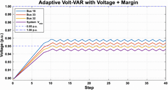
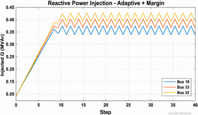
Figure 12 shows the iteration-wise voltage evolution under adaptive gain-scheduled control. The adaptive controller raises the minimum voltage to approximately 0.9491 per unit and reduces the number of buses below 0.95 per unit more strongly than the traditional controller. Figure 13 shows the reactive-power commands generated by the adaptive controller.
Figure 12. Voltage regulation response for controlled buses using adaptive gain-scheduled control
Figure 13. Reactive power injection control dynamics with adaptive gain-scheduled control
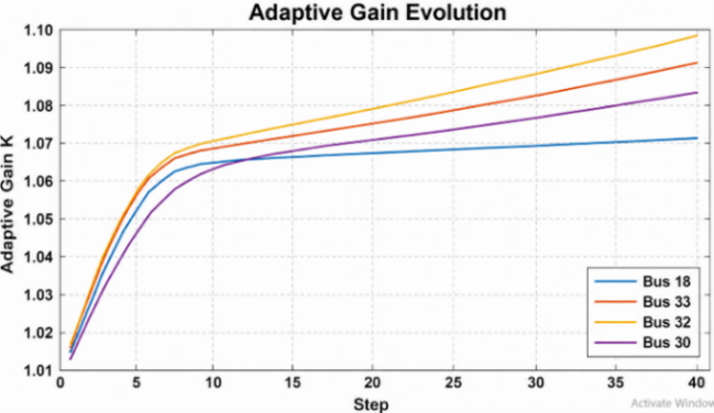
The adaptive strategy supplies slightly stronger reactive-power support at the more weakly regulated buses, consistent with the gain increase produced by the local voltage-error rule. Figure 14 shows how the bounded adaptive gain changes across control iterations. From Figure 14, it is observed that the adaptive gain increases from K = 1.01 to about K = 1.09, indicating online adaptive tuning of gain in the controller.
Figure 14. Adaptive gain-scheduling response for online implementation under the suggested controller
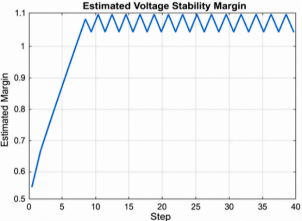
Figure 15 shows the plot of control actions and the stability margin of voltage under adaptive gain-scheduled Volt-VAR controller.
Figure 15. Voltage stability margin dynamic response under gain-scheduled adaptive control
From Figure 15, the stability margin estimates increased from about 0.55 to greater than 1.0, suggesting that there have been significant improvements to voltage stability under adaptive control. Table 4 gives the result of adaptive Volt-VAR control and stability margin superiority.
Table 4. Results after implementation of adaptive Volt-VAR control and stability margin supervision
|
Performance Index |
Final Value |
|
Final minimum voltage bus |
Bus 13 |
|
Final minimum voltage |
0.949120 p.u. |
|
Final buses below 0.95 p.u. |
3 |
|
Final real power loss |
0.188652 MW |
|
Final reactive power loss |
0.129393 MVAr |
|
Final estimated stability margin |
1.098084 |
Table 5 final controlled-bus voltages, reactive power injection, and adaptive gains with respect to control bus. Relative to traditional control, the adaptive controller increases Vmin from 0.9481 to 0.949120 p.u., reduces buses below 0.95 p.u. from 6 to 3, and raises the estimated stability margin from 1.0847 to 1.098084. The stronger voltage support is accompanied by small increases in active loss from 0.1868 to 0.188652 MW and reactive loss from 0.1278 to 0.129393 MVAr. Thus, the principal adaptive benefit is broader voltage recovery and a higher estimated margin, with a small loss trade-off.
Table 5. Final controlled-bus voltages, reactive power injection, and adaptive gains
|
Control Bus |
Final Voltage (p.u.) |
Injected Q )MVAr( |
Adaptive Gain K |
|
18 |
0.953534 |
0.371394 |
1.070146 |
|
33 |
0.952212 |
0.408497 |
1.084813 |
|
32 |
0.951103 |
0.422472 |
1.091193 |
|
16 |
0.952637 |
0.400000 |
1.080523 |
|
30 |
0.949474 |
0.438535 |
1.092206 |
5.6 Comparative performance evaluation for traditional and adaptive controllers
Table 6 summarizes the differences between traditional and adaptive controllers under the same stressed condition—minimum voltage, weak-bus count, power-loss changes, and estimated stability margin—and shows the improvement ratio of the adaptive method over the traditional one.
Table 6. Final improvement of adaptive control over traditional control
|
Performance Index |
Improvement of Adaptive over Traditional |
|
Minimum Voltage |
0.1%+ |
|
Weak Buses |
Reduction 50% |
|
Active Power Loss |
Increase 0.99% |
|
Reactive Power Loss |
Increase 1.25% |
|
Stability Margin |
1.23%+ |
|
Weakest Bus |
Support maintained at Bus 13 |
5.6.1 Comparative discussion
The adaptive increase in minimum voltage is modest (about +0.11%), but the number of buses below 0.95 p.u. is halved from 6 to 3 and the estimated stability margin rises by about 1.23%. These gains are obtained with approximately 0.99% higher active loss and 1.25% higher reactive loss than traditional control. This behavior is consistent with the gain-scheduling mechanism: larger voltage error increases K and therefore reactive-power support, whereas the gain relaxes as voltage improves. The present MATPOWER trajectories are iterative/quasi-static; the systematic comparison under different loading conditions is reported in Section 5.8.
5.7 Sensitivity analysis of controller parameters
To test the robustness of the designed controller, a sensitivity analysis has been done considering the main controller parameters Qmax. One of the parameters was varied at a time while holding all the other parameters fixed for comparison.
5.8 Performance validation under different stress conditions
To evaluate controller robustness under changing operating stress, the traditional and adaptive controllers were tested at load factors of 1.05, 1.10, and 1.15 while retaining the same IEEE 33-bus network, control buses [16, 18], Volt-VAR breakpoints, reactive-power limits, rate limit, downstream stress factor, and controller tuning. No retuning was performed between scenarios. The results are summarized in Table 7. At a load factor of 1.05, the adaptive controller increased the minimum voltage from 0.945943 to 0.951167 p.u., eliminated all buses below 0.95 p.u. (14 to 0), and increased the estimated margin from 1.048996 to 1.115864, although active and reactive losses increased slightly. At the main stressed condition of 1.10, the adaptive controller again improved the minimum voltage from 0.948096 to 0.949120 p.u., reduced buses below 0.95 p.u. from 6 to 3, and increased the estimated margin from 1.084728 to 1.098084, with small increases in power losses. Under the more severe 1.15 loading condition, however, the adaptive controller did not outperform the traditional controller in the voltage-stability indicators: the minimum voltage decreased from 0.945976 to 0.942921 p.u., the number of buses below 0.95 p.u. increased from 12 to 16, and the estimated margin decreased from 1.066448 to 1.026634. In this severe case, the adaptive controller instead produced lower active and reactive losses than the traditional controller. These results show that the benefit of the proposed adaptive strategy is operating-point dependent rather than uniformly superior over the full tested stress range. The high-stress result is therefore treated as a limitation of the present gain-scheduling and supervisory settings and indicates that more robust parameter scheduling or online retuning may be required for more severe loading conditions.
Table 7. Performance of traditional and adaptive controllers under different loading levels
|
Load factor Controller |
Vmin (p.u.) N < 0.95 |
Ploss (MW) Qloss (MVAr) |
Estimated Margin |
|
1.05 Traditional |
0.94594314 |
0.163814 0.110904 |
1.048996 |
|
1.05 Adaptive |
0.9511670 |
0.170083 0.116503 |
1.115864 |
|
1.10 Traditional |
0.9480966 |
0.186787 0.127817 |
1.084728 |
|
1.10 Adaptive |
0.9491203 |
0.188652 0.129393 |
1.098084 |
|
1.15 Traditional |
0.94597612 |
0.206152 0.141216 |
1.066448 |
|
1.15 Adaptive |
0.94292116 |
0.201028 0.136803 |
1.026634 |
This paper presented a comparative evaluation of traditional and adaptive gain-scheduled Volt-VAR controllers for improving voltage stability in the IEEE 33-bus radial distribution network. Under the stressed operating condition, the system suffered from undervoltage, with a minimum bus voltage of 0.9038 p.u. and 21 buses below the acceptable limit of 0.95 p.u. The V-Q modal analysis and CPF results also confirmed weak voltage stability, with Bus 18 identified as the critical bus. Both controllers improved the system performance; however, the adaptive controller achieved better results, increasing the minimum voltage to 0.9491 p.u., reducing the number of weak buses from 21 to 3, and raising the estimated stability margin to 1.0981. Compared with the conventional controller, the adaptive controller reduced the weak buses by about 50%, representing the most significant improvement, although the reactive power loss showed a slight increase of +1.25%. To verify controller robustness and justify the selected parameters, a sensitivity analysis was carried out for the main controller parameter Qmax, by changing one parameter at a time while keeping the other operating conditions fixed. The evaluation was taken minimum voltage, number of weak buses, active power losses, and estimated stability margin.
Practical implementation of the adaptive method requires reliable voltage measurements, sufficient inverter reactive-power headroom, and access to the supervisory stability-margin estimate. If the margin is evaluated centrally, telemetry and communication are also required, which introduces additional implementation and maintenance cost. Stronger reactive-power operation can also increase converter utilization. Moreover, the present validation is limited to the IEEE 33-bus benchmark; larger-network and time-domain or hardware-in-the-loop validation are therefore identified as future work.
Table 8 summarizes the quantitative performance of the adaptive controller relative to the traditional controller in terms of voltage improvement, reduction in the number of weak buses, active and reactive power losses, estimated stability margin, and weakest-bus location.
Table 8. Quantitative summary of adaptive control relative to traditional control
|
Performance Metric |
Adaptive Relative to Traditional |
|
Minimum voltage |
+0.11% |
|
Buses below 0.95 p.u. |
50% reduction (6 → 3) |
|
Active power loss |
0.99% increase |
|
Reactive power loss |
1.25% increase |
|
Estimated stability margin |
+1.23% (1.0847 → 1.0981) |
|
Weakest bus |
Bus 13 in both controlled cases |
|
Bij |
Susceptance element between buses i and j, p.u. |
|
e(k) |
Voltage error at control step k, p.u. |
|
Gij |
Conductance element between buses i and j, p.u. |
|
J |
Newton-Raphson Jacobian matrix, dimensionless |
|
J1, J2, J3, J4 |
Submatrices of the Newton-Raphson Jacobian, dimensionless |
|
JR |
Reduced Jacobian matrix used in V-Q modal analysis, dimensionless |
|
K(k) |
Adaptive gain at control step k, dimensionless |
|
M(k) |
Estimated voltage stability margin at control step k, dimensionless |
|
N (V<0.95) |
Number of buses with voltage lower than 0.95 p.u., dimensionless |
|
Pi |
Active power injection at bus i, MW |
|
PD(λ) |
Active load demand as a function of loading factor, MW |
|
PD0 |
Base active load demand, MW |
|
Ploss |
Total active power loss, MW |
|
Qi |
Reactive power injection at bus i, MVAr |
|
Qadp(k) |
Adaptive reactive power command at control step k, MVAr |
|
QD(λ) |
Reactive load demand as a function of loading factor, MVAr |
|
QD0 |
Base reactive load demand, MVAr |
|
Qloss |
Total reactive power loss, MVAr |
|
Qmax |
Maximum reactive power limit, MVAr |
|
Qmin |
Minimum reactive power limit, MVAr |
|
Qraw(k) |
Raw reactive power command before final limiting, MVAr |
|
Qvv(k) |
Reactive power output from the Volt-VAR characteristic, MVAr |
|
Vi |
Voltage magnitude at bus i, p.u. |
|
Vj |
Voltage magnitude at bus j, p.u. |
|
Vbase |
Base-case voltage value, p.u. |
|
Vmin |
Minimum bus voltage magnitude in the system, p.u. |
|
Vnew |
Voltage value after applying control or compensation, p.u. |
|
Vnose |
Voltage magnitude at the nose point of the P-V curve, p.u. |
|
Vref |
Reference voltage used by the controller, p.u. |
|
K0 |
Nominal adaptive gain, dimensionless |
|
Kmin |
Minimum adaptive gain, dimensionless |
|
Kmax |
Maximum adaptive gain, dimensionless |
|
ehigh |
High voltage-error threshold used in gain-scheduling, p.u. |
|
elow |
Low voltage-error threshold used in gain-scheduling, p.u. |
|
Vdb,low |
Lower adaptive-gain deadband boundary, p.u. |
|
Vdb,high |
Upper adaptive-gain deadband boundary, p.u. |
|
Mlow |
Lower supervisory stability-margin threshold, dimensionless |
|
Mmid |
Intermediate supervisory stability-margin threshold, dimensionless |
|
Greek symbols |
|
|
βmargin(k) |
Supervisory stability-margin modulation factor at control step k, dimensionless |
|
ΔP |
Active power mismatch vector in Newton-Raphson load flow, MW |
|
ΔQ |
Reactive power mismatch vector or reactive power change, MVAr |
|
ΔQmax |
Maximum allowable change in reactive power per control step, MVAr |
|
ΔV |
Voltage magnitude correction vector, p.u. |
|
Δθ |
Voltage angle correction vector, rad |
|
θij |
Voltage angle difference between buses i and j, rad |
|
λ |
Loading factor used in continuation power flow, dimensionless |
|
λmax |
Maximum loading factor or loadability limit, dimensionless |
|
λmin |
Smallest eigenvalue of the reduced Jacobian matrix, dimensionless |
|
φi |
Right eigenvector associated with mode i, dimensionless |
|
βhigh |
Supervisory multiplier for low-margin conditions, dimensionless |
|
βmid |
Supervisory multiplier for intermediate-margin conditions, dimensionless |
|
βnom |
Nominal supervisory multiplier, dimensionless |
|
γup |
Adaptive-gain increase coefficient, dimensionless |
|
γdown |
Adaptive-gain decrease/relaxation coefficient, dimensionless |
|
Subscripts |
|
|
adp |
Adaptive control quantity |
|
base |
Base-case value |
|
D |
Demand or load quantity |
|
i, j |
Bus indices |
|
inj |
Injected quantity |
|
k |
Control step or iteration index |
|
loss |
Power loss quantity |
|
max |
Maximum value |
|
min |
Minimum value |
|
new |
Value after control or compensation |
|
raw |
Unconstrained control command before limiting |
|
ref |
Reference value |
|
vv |
Volt-VAR control quantity |
[1] Euldji, Ndlela, N.W., Moloi, K., Kabeya, M. (2025). High-penetration of renewable energy into the grid. MDPI AG. https://doi.org/10.20944/preprints202507.1440.v1
[2] Adetokun, B.B., Muriithi, C.M., Ojo, J.O., Oghorada, O. (2023). Impact assessment of increasing renewable energy penetration on voltage instability tendencies of power system buses using a QV-based index. Scientific Reports, 13(1). https://doi.org/10.1038/s41598-023-36843-5
[3] Photovoltaics, D.G., Storage, E. (2018). IEEE standard for interconnection and interoperability of distributed energy resources with associated electric power systems interfaces. IEEE Std 1547-2018 (Revision of IEEE Std 1547-2003). https://doi.org/10.1109/IEEESTD.2018.8332112
[4] Werkie, Y.G., Nyakoe, G.N., Wekesa, C.W. (2025). Voltage stability assessment based on modified line voltage stability index in the presence of renewable energy integration and credible contingencies. Engineering Reports, 8: e70578. https://doi.org/10.1002/eng2.70578
[5] Mokred, S., Wang, Y., Alruwaili, M., Ibrahim, M.A. (2025). A novel approach for voltage stability assessment and optimal siting and sizing of DGs in radial power distribution networks. Processes, 13(7): 2239. https://doi.org/10.3390/pr13072239
[6] Mokred, S., Wang, Y. (2025). Comparative analysis of voltage stability in radial power distribution networks under critical loading conditions and diverse load models. Electricity, 6(4): 64. https://doi.org/10.3390/electricity6040064
[7] Barnwal, A.K., Yadav, L.K., Verma, M.K. (2022). A multi-objective approach for voltage stability enhancement and loss reduction under PQV and P buses through reconfiguration and distributed generation allocation. IEEE Access, 10: 16609-16623. https://doi.org/10.1109/access.2022.3146333
[8] Ren, H., Jha, R.R., Dubey, A., Schulz, N.N. (2021). Extremum-seeking adaptive-droop for model-free and localized volt-var optimization. IEEE Transactions on Power Systems, 37(1): 179-190. https://doi.org/10.1109/TPWRS.2021.3093831
[9] Arnold, D., Saha, S., Ngo, S.T., et al. (2023). Adaptive control of distributed energy resources for distribution grid voltage stability. IEEE Transactions on Power Systems, 38(1): 129-141. https://doi.org/10.1109/tpwrs.2022.3157558
[10] Cheng, R., Shi, N., Maharjan, S., Wang, Z. (2023). Automatic self-adaptive local voltage control under limited reactive power. IEEE Transactions on Smart Grid, 14(4): 2851-2862. https://doi.org/10.1109/tsg.2022.3224463
[11] Lumina, S.D., Mnguni, M.E., Mfoumboulou, Y.D. (2023). Photovoltaic controller design based on adaptive volt/var algorithm to stand the impact of load increase in grid tied microgrid system. International Journal of Electrical and Electronic Engineering & Telecommunications, 12(3): 186-193.
[12] Murzakhanov, I., Gupta, S., Chatzivasileiadis, S., Kekatos, V. (2024). Optimal design of Volt/VAR control rules for inverter-interfaced distributed energy resources. IEEE Transactions on Smart Grid, 15(1): 312-323. https://doi.org/10.1109/tsg.2023.3279982
[13] Doni, D., Gianto, R., Abidin, Z. (2024). Voltage stability index improvement in radial distribution systems using capacitors. Journal of Electrical Engineering, Energy, and Information Technology (J3EIT), 12(1): 342-354.
[14] Zimmerman, R.D., Murillo-Sánchez, C.E. (2025). MATPOWER user’s manual. Zenodo. https://doi.org/10.5281/ZENODO.15871661
[15] Kwangkaew, A., Javaid, S., Charoenlarpnopparut, C., Kaneko, M. (2022). Optimal location and sizing of renewable distributed generators for improving voltage stability and security considering reactive power compensation. Energies, 15(6): 2126. https://doi.org/10.3390/en15062126
[16] Raza, A., Zahid, T., Iqbal, S., Ahmad, I., Hussain, J. (2024). Optimizing power flow: A study of Newton Raphson (NR) method for load flow analysis (LFA) in power systems. Innovative Computing Review, 4(1): 37-50. https://doi.org/10.32350/icr.41.03
[17] Liang, X., Chai, H., Ravishankar, J. (2022). Analytical methods of voltage stability in renewable dominated power systems: A review. Electricity, 3(1): 75-107. https://doi.org/10.3390/electricity3010006
[18] Ogata, K. (1996). Modern Control Engineering, 3rd ed. Prentice Hall.
[19] Choden, K., Tenzin, S., Seldon, Y. (2022). Enhancement of voltage stability in the power system using genetic algorithm. Journal of Applied Engineering, Technology and Management, 2(1): 65-77. https://doi.org/10.54417/jaetm.v2i1.59
[20] Shakeel, M., Uppal, A., Tasneem, N., Alsmadi, Y. (2026). Optimization of distributed energy resources in distribution networks using multi-objective Archimedes optimization algorithm. Symmetry, 18(1): 75. https://doi.org/10.3390/sym18010075