Osman Doğuş Gülgün* | Hamza Erol
© 2026 The authors. This article is published by IIETA and is licensed under the CC BY 4.0 license (http://creativecommons.org/licenses/by/4.0/).
OPEN ACCESS
Diabetic retinopathy (DR) is a common eye disease in which vision loss can be prevented through early diagnosis. However, the manual assessment of fundus images is time-consuming and observer-dependent. In this study, four established feature selection methods from different approaches are systematically compared in terms of their ability to reduce deep features to compact representations in the binary classification of DR from fundus images. On the Asia Pacific Tele-Ophthalmology Society (APTOS) 2019 dataset, four ImageNet-pretrained convolutional neural networks (CNNs) (EfficientNet-B1, DenseNet-121, ResNet-50, and ConvNeXt-Tiny) were fine-tuned to extract deep features. Following a variance-thresholding pre-filter, the extracted features were reduced using these four feature selection methods (Boruta, minimum redundancy maximum relevance (mRMR), Lasso, and random forest importance (RFI)) and fed into a four-layer artificial neural network (ANN) classifier. The main configuration, obtained by combining EfficientNet-B1 with RFI, reduced the feature dimensionality from 1,280 to 94, achieving 99.45% accuracy and an area under the curve (AUC) of 0.9997, and improving on the fine-tuning-only models. The applied feature selection approach yielded consistent performance across the four tested architectures. Overall, the proposed approach shows that a compact subset of the deep features is sufficient for high-performance binary DR classification.
binary classification, convolutional neural network, deep learning, diabetic retinopathy, feature selection, fundus imag
Diabetic retinopathy (DR) is a progressive disease that arises from the damage caused by prolonged high blood sugar to the fine blood vessels in the retina and is regarded as one of the most common ocular complications of diabetes [1]. Usually asymptomatic in its early stages, DR manifests in its advancing stages with findings such as microaneurysms, hemorrhages, and exudates in the retina. In its advanced stages, more serious signs such as neovascularization and intraocular hemorrhages emerge. When left untreated, the disease can lead to irreversible vision loss [2]. The increasing prevalence of the disease with the duration of diabetes, its place among the leading causes of preventable blindness in the working-age population, and the steadily growing number of diabetic patients worldwide continually heighten the importance of the early and accurate diagnosis of DR [3].
In clinical practice, the diagnosis of DR mostly relies on the visual assessment performed by expert ophthalmologists on color fundus images. When necessary, this diagnosis is supported by advanced imaging techniques such as optical coherence tomography and fundus fluorescein angiography [4]. Owing to its non-invasive nature, relatively low cost, and wide availability, fundus imaging is regarded as the fundamental tool, particularly in screening programs. Nevertheless, the difficulty of detecting early-stage findings such as microaneurysms and small hemorrhages, the variability in image quality, inter-observer differences, and the insufficient number of expert ophthalmologists, especially in low- and middle-income regions, render the manual assessment process time-consuming, laborious, and error-prone. This situation markedly increases the need for artificial intelligence-based decision-support systems that can enable the automatic detection of DR so that large numbers of fundus images can be evaluated rapidly and consistently.
In recent years, deep learning-based methods have come to the fore with the high accuracy and generalizability they provide in classification, lesion detection, and disease grading problems in medical images [5]. In particular, convolutional neural networks (CNNs) have enabled the automatic modeling of DR-specific findings in fundus images. Through the use of CNN architectures together with transfer learning, attention mechanisms, and advanced data augmentation strategies, the literature has begun to offer a reliable basis for clinical decision-support systems [6].
In this context, numerous deep learning approaches have been introduced in the literature for the diagnosis of DR through binary classification from fundus images. These studies have largely centered on the comparison of pretrained CNN architectures, the selection of deep features, and compact classification. Beyond these, transformer-based and attention-based architectures and systems evaluated under real clinical conditions have also drawn attention in the literature.
Studies that comparatively evaluate pretrained CNN architectures for DR binary classification occupy an important place in the literature. Saproo et al. [7] systematically compared 20 different pretrained networks under three architectural categories in the context of DR binary classification. For the training and validation of the models, the DRD-EyePACS, Indian Diabetic Retinopathy Image Dataset (IDRiD), and Asia Pacific Tele-Ophthalmology Society (APTOS) 2019 datasets were combined to form a dataset of 6,928 images. On this dataset, the highest performance was obtained with ResNet-101, at 97.33% accuracy.
Youldash et al. [8] compared the performances of six modern pretrained CNNs selected from the EfficientNet and RegNet families in DR binary classification. The models were evaluated through transfer learning both on the APTOS 2019 dataset and on a clinical dataset compiled from the Al-Saif Medical Center in Saudi Arabia. On APTOS 2019, the highest accuracy of 98.60% was obtained with RegNet-X080. In cross-center validation, the EfficientNet-B3 model reached a binary classification accuracy of 98.20%.
Anand et al. [9] compared the EfficientNet-B0, ResNet-152, VGG-16, and DenseNet-169 pretrained models in the context of DR binary classification. In this comparison, a common fine-tuning block consisting of global average pooling, flattening, dropout, and dense layers was added to the models so that the evaluation was performed under the same conditions. On a dataset of 3,200 images acquired with three different fundus cameras, the best result was obtained with EfficientNet-B0, yielding 91% accuracy and a 0.90 area under the curve (AUC).
However, these comparative studies use the raw deep features of the networks directly, without applying feature selection to obtain more compact and discriminative representations.
Another line of research applies feature selection or reduction to the features used for DR binary classification, sometimes fusing features obtained from multiple networks. In this regard, Rahman et al. [10] proposed a hybrid approach on the APTOS 2019 dataset. In their method, a multi-stage preprocessing consisting of contrast-limited adaptive histogram equalization (CLAHE), Lab color space conversion, and green channel extraction was applied, after which the features obtained with ResNet-50 were reduced through principal component analysis. The reduced features were evaluated with support vector machine (SVM), k-nearest neighbors, and Histogram Gradient Boosting classifiers, and the highest accuracy of 96.90% was obtained with SVM.
Butt et al. [11] developed a hybrid feature framework based on combining features extracted from different CNN architectures. In their approach, the feature vectors obtained from the ImageNet-pretrained GoogLeNet and ResNet-18 networks were concatenated to form a hybrid vector. This vector was evaluated by feeding it into SVM, Random Forest, Radial Basis Function, and Naive Bayes classifiers. On APTOS 2019, the best result was obtained with the SVM-based hybrid structure, yielding 97.80% accuracy and balanced sensitivity-specificity values.
Sapra et al. [12] proposed an approach that optimizes feature selection in the binary classification of DR. In their method, correlation-based feature subset selection searched using particle swarm optimization was combined with information gain-based filtering through a union operation to obtain an optimized feature set, and these features were classified with a five-layer sequential deep neural network. An accuracy of 93.5% was obtained on the Diabetic Retinopathy Debrecen dataset, which is derived from Messidor images and consists of 1,151 records with 20 features.
However, these studies each adopt a single strategy and do not compare methods from different approaches on the same deep features.
Compact classification, which aims to lower model complexity and computational cost, forms another prominent direction in DR binary classification. Zafar et al. [13] designed a lightweight CNN architecture containing only approximately 1.3 million learnable parameters and consisting of 37 layers with a single parallel branch. The proposed architecture was positioned within a two-stage framework. In the first stage, the binary detection of DR was performed, while in the second stage, a multi-class staging task was carried out through transfer learning. On APTOS 2019, 99.06% accuracy and a 0.98 Cohen kappa score were obtained in binary detection. This result demonstrated that high performance can be achieved with a low parameter cost compared with much larger models.
In a similar direction, Liu et al. [14] proposed a new attention module based on the agent attention mechanism, an efficient attention approach, in order to reduce the quadratic computational complexity of the classical self-attention mechanism. This module was integrated into the vision transformer (ViT) architecture, enabling the simultaneous modeling of both global and local features. On binary lesion classification on Messidor, a 0.973 AUC, 96.90% accuracy, and a 94.70% F1-score were obtained.
However, these approaches pursue compactness through lightweight architectures rather than through the selection of a compact subset of deep features.
Apart from these three directions, studies such as specialized dual-branch architectures [15], transformer-based and attention-based models [16, 17], and systems validated in real clinical settings [18] have also made important contributions to the DR binary classification literature.
The existing literature clearly reveals that deep learning-based methods can provide high performance in the binary classification of DR from fundus images. However, these directions have largely been pursued in isolation, rather than within a single evaluation that connects feature selection, deep representations, and compactness.
In this study, in order to address this gap, feature selection methods from different approaches are systematically compared on deep features within a common evaluation framework for DR binary classification using the APTOS 2019 dataset. This study makes four main contributions: (i) the formation of a two-stage selection process in which a common variance-thresholding pre-filter is applied before feature selection methods belonging to different approaches, (ii) the systematic comparison of the deep features extracted from modern CNN architectures within this selection process, (iii) the demonstration of the contribution of feature selection to classification performance by comparing the proposed approach with the CNN models trained only with fine-tuning, and (iv) the reduction of the high-dimensional deep features to a compact representation while preserving classification performance.
In the proposed approach, after CLAHE-based preprocessing and moderate data augmentation, four modern CNN architectures (EfficientNet-B1, DenseNet-121, ResNet-50, and ConvNeXt-Tiny) are fine-tuned to extract deep features. These features, after a common variance-thresholding step, are reduced separately with the Boruta, minimum redundancy maximum relevance (mRMR), Lasso, and random forest importance (RFI) methods, which represent four different approaches, and are classified with an artificial neural network (ANN).
In the remainder of the study, the dataset used, the preprocessing stages, the proposed method, and the experimental setup are presented in detail. On the APTOS 2019 dataset, the proposed main configuration was formed by combining EfficientNet-B1 with RFI. This configuration reached 99.45% accuracy and a 0.9997 AUC using only 94 features. The obtained results are discussed in comparison with the existing literature.
This section presents in detail the proposed approach for the binary classification of DR from fundus images. The proposed approach is organized into six subsections comprising the dataset, data preprocessing, model architecture, training process, development environment, and evaluation metrics.
2.1 Dataset
In this study, the APTOS 2019 fundus image dataset, compiled within the scope of the competition organized by APTOS and published on the Kaggle platform in 2019, was used [19]. The dataset consists of 3,662 colour fundus images acquired in different clinical settings; the images exhibit substantial differences in terms of resolution, brightness, and image quality. This diversity ensures that the variability encountered in real clinical conditions is represented to a considerable extent.
In the original dataset, each image was labelled by expert ophthalmologists into one of five distinct classes according to DR severity. These classes were defined as Normal (0), Mild DR (1), Moderate DR (2), Severe DR (3), and Proliferative DR (4). Since this study targets the binary classification of DR, this five-class structure was converted into a binary label scheme. Within this conversion, images labelled 0 were assigned to the “Normal” class, whereas images labelled 1, 2, 3, and 4 were assigned to the “DR” class. In line with the established approach in clinical screening applications, the positive class was defined as the DR class, which represents the presence of disease.
The dataset was obtained from a publicly available version on Kaggle in which it is already partitioned into training, validation, and test subsets [20]. In this study, this partition was preserved as is, and no additional splitting was performed. The training, validation, and test subsets consist of 2,930, 366, and 366 images, respectively. After the binary label conversion was applied, the training subset comprises 1,496 DR and 1,434 Normal images, the validation subset comprises 194 DR and 172 Normal images, and the test subset comprises 167 DR and 199 Normal images.
2.2 Data preprocessing
This section describes the image preprocessing and data augmentation steps applied to the fundus images. These steps were systematically designed and applied in order to improve image quality, strengthen the learning process of the model, and limit the tendency toward overfitting.
2.2.1 Fundus region cropping and contrast-limited adaptive histogram equalization
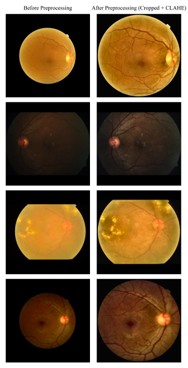
Since the images in the APTOS 2019 dataset were captured with different cameras, wide black background regions surround the fundus tissue in the images. This causes both the fundus tissue to remain relatively small and the image contrast to weaken. To overcome this limitation, a two-step preprocessing pipeline was applied.
In the first step, the black background of each image was cropped to isolate the fundus region. Within this process, the image was first converted to grayscale; exploiting the fact that the background pixels have near-zero values, a binary mask separating the fundus region from the background was created using a fixed threshold at an intensity of 10; this mask was cleaned of small gaps and noise through morphological closing and opening operations using an elliptical structuring element (15 × 15); and the bounding box determined from the resulting mask was cropped, leaving a 1% margin. Through this step, the model was enabled to focus on the fundus region rather than the background.
In the second step, CLAHE was applied to improve the local contrast characteristics of the cropped images [21]. Within this scope, the image was converted from the red–green–blue (RGB) color space to the CIELAB (Lab) color space; then CLAHE was applied to the L channel, which carries the brightness information. The CLAHE parameters were set as a clip limit of 2.0 and a tile grid size of 8 × 8. The processed L channel was recombined with the A and B channels, and the image was converted back to the RGB color space. This preprocessing pipeline enhanced the visibility of low-contrast lesions, in particular microaneurysms, small vascular irregularities, and exudates, and provided a suitable basis for the deep learning-based feature extraction performed in the subsequent stage. The parameter values used in these preprocessing steps were determined through preliminary experiments and kept fixed throughout the study. Representative fundus images with different visual characteristics, selected from the APTOS 2019 dataset, are shown before and after the proposed preprocessing steps in Figure 1.
Figure 1. Representative fundus images with different visual characteristics from the Asia Pacific Tele-Ophthalmology Society (APTOS) 2019 dataset before (left) and after (right) applying the proposed preprocessing steps
2.2.2 Data augmentation
Although there is no marked imbalance between the DR and Normal classes in the APTOS 2019 dataset, a moderate data augmentation strategy was adopted in order to increase the diversity of learning during the training phase of the model and to limit the tendency toward overfitting. Within this scope, data augmentation was applied only to the training subset; the validation and test subsets were preserved in their original form. This approach ensures that the validation and test results are evaluated only on real data.
The applied data augmentation steps consist of horizontal flipping (application probability 0.5), small-angle geometric transformation (rotation angle ±8°, shift ratio ±5%, scale factor ±5%, application probability 0.7), and slight brightness and contrast variation (brightness variation ratio ±8%, contrast variation ratio ±8%, application probability 0.4). These steps were applied offline before the training process using the Albumentations library [22].
In the data augmentation process, the number of images in the training subset of each class was balanced to a target of 2,000. Within this scope, 504 new images were added to the 1,496 original images in the DR class, and 566 new images were added to the 1,434 original images in the Normal class. As a result, the training subset was turned into a balanced set consisting of a total of 4,000 images, containing 2,000 images from each of the DR and Normal classes.
2.3 Proposed two-stage feature selection-based classification approach
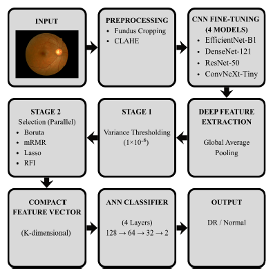
This section explains in detail the proposed approach for the binary classification of DR from fundus images. The proposed approach consists of three main components: extracting deep features using a modern CNN backbone, passing the extracted features through a two-stage selection process, and classifying the selected compact feature set by means of an ANN classifier. The general flow diagram of this approach is presented in Figure 2.
Figure 2. Flow diagram of the proposed two-stage feature selection-based classification approach
2.3.1 Convolutional neural network fine-tuning and deep feature extraction
In the deep feature extraction stage, four modern CNN architectures representing different design approaches were used. These architectures were selected as EfficientNet-B1, designed with a compound scaling approach; DenseNet-121, based on a dense connectivity structure; ResNet-50, distinguished by deep residual connections; and ConvNeXt-Tiny, developed by drawing inspiration from transformer architectures [23-26]. All models were initialized with weights pretrained on the ImageNet dataset [27].
The original classifier layer of each CNN architecture was replaced with a two-output linear layer, appropriate for the binary classification task. All of the models were fine-tuned end-to-end on the training subset. During fine-tuning, all parameters of the models were updated; in this way, the models were enabled to learn discriminative patterns specific to DR.
After fine-tuning was completed, deep feature extraction was performed for each CNN, separately for the training, validation, and test subsets. Within this scope, the final classifier layer of the CNNs was replaced with the identity function; thus, direct access to the high-dimensional feature vectors obtained from the output of the global average pooling layer was provided. The dimensions of these vectors were 1,280 for EfficientNet-B1, 1,024 for DenseNet-121, 2,048 for ResNet-50, and 768 for ConvNeXt-Tiny, respectively. The number of parameters of these architectures is approximately 7.8 M, 8.0 M, 25.5 M, and 28.5 M, respectively.
2.3.2 Two-stage feature selection
In order to increase the performance of the classification process performed on the deep features and to obtain a more compact feature representation, a two-stage feature selection procedure was designed. This procedure was applied in a common manner to the features extracted from all CNN architectures. Throughout this procedure, all selection steps were fitted only on the training features, and the resulting feature subsets were then applied to the validation and test features, which were not used when fitting these steps.
In the first stage, the extracted features were passed through a common variance thresholding step. In this step, the threshold value was set to 1 × 10⁻⁶, and features whose variance was below this threshold were eliminated. Because such features are nearly constant across the samples, they contribute little to the discrimination between the classes. This pre-filtering step ensured that the feature selection methods applied in the subsequent stage operated on a more compact feature set and increased the stability of the selection process.
In the second stage, four feature selection methods belonging to different approaches were applied in parallel to the features that passed the variance thresholding. These methods were determined as Boruta, representing the wrapper approach; mRMR, representing the filter approach; Lasso, representing the embedded approach; and RFI, representing the tree-based approach. This choice enables the four fundamental approaches in the feature selection literature to be systematically compared on the same classification infrastructure. Apart from the variance thresholding, no further standardization was applied to the features before selection. The only exception was the Lasso method, for which the features were standardized to zero mean and unit variance on the training set, since L1-regularized logistic regression is sensitive to feature scaling.
The Boruta method [28] is a wrapper approach that makes use of the Random Forest algorithm. At the core of the method lies the comparison of the values of the original features with their randomly reshuffled copies, referred to as shadow features. When a feature has an importance value statistically significantly higher than the highest importance of the shadow features, that feature is considered confirmed and included in the selected set [29]. In this study, the Boruta procedure was based on a Random Forest with 200 trees, was run for a maximum of 50 iterations, and used a significance level of 0.05.
The mRMR method [30] is a feature selection algorithm based on the filter approach. This method highlights features that have high relevance to the target label but low redundancy among themselves. In this study, feature relevance was quantified with the F-statistic and feature redundancy with the Pearson correlation coefficient. The maximum selection size of the mRMR method was set to 200, and an adaptive cutoff eliminated the features remaining below 30% of the highest relevance value [31].
The Lasso method [32] was applied as an example of the embedded approach. In this method, a logistic regression model with L1 regularization was trained; the features corresponding to the coefficients that were not set to zero during the training process were included in the selected set. The L1 regularization strength was determined through 3-fold cross-validation over the candidate values 0.001, 0.01, 0.1, 1, and 10 [33].
The RFI method [34] was applied as the representative of the tree-based approach. In this method, a Random Forest classifier with 200 trees was trained; the importance scores were calculated based on the contribution of each feature to reducing the Gini impurity. Features whose importance score remained above the mean value of all features were included in the selected set [35].
The threshold values described above were set through preliminary experiments and were kept unchanged across all configurations. Summary information of the feature selection methods is presented in Table 1.
Table 1. Method summary of the proposed two-stage feature selection procedure
|
Stage |
Method |
Approach |
Thresholding Mechanism |
|
1 |
Variance Thresholding |
Pre-filtering |
Fixed threshold (1 × 10⁻⁶) |
|
2 |
Boruta |
Wrapper |
Shadow feature comparison |
|
2 |
mRMR |
Filter |
Adaptive cutoff (30% of the highest relevance) |
|
2 |
Lasso |
Embedded |
L1 regularization (cross-validated coefficient) |
|
2 |
RFI |
Tree-based |
Above the mean importance score |
2.3.3 Artificial neural network classifier
The compact feature subset obtained in the second stage was fed into a four-layer ANN classifier trained independently for each CNN architecture. This ANN classifier was designed as an architecture containing regularization layers aimed at limiting the tendency of the model toward overfitting.
In the ANN architecture, the input vector first passes through a batch normalization (BN) layer, then through three hidden layers consisting of 128, 64, and 32 neurons, respectively, reaching the two-class output in the final layer. At the output of each hidden layer, BN, the rectified linear unit (ReLU) activation function, and dropout are applied. The dropout probability was set to 0.3, 0.3, 0.2, and 0.1 from the input layer toward the final layer, respectively. Thanks to the regularization layers, overfitting of the model on the high-dimensional input is limited. The layer structure of the proposed ANN classifier is presented in Table 2.
Table 2. Layer structure of the proposed artificial neural network (ANN) classifier
|
Layer |
Output Size |
Components |
|
Input |
K |
Compact feature vector (K varies by CNN and method) |
|
Normalization + Dropout |
K |
BN, Dropout (0.3) |
|
Hidden Layer 1 |
128 |
Linear + BN + ReLU + Dropout (0.3) |
|
Hidden Layer 2 |
64 |
Linear + BN + ReLU + Dropout (0.2) |
|
Hidden Layer 3 |
32 |
Linear + BN + ReLU + Dropout (0.1) |
|
Output |
2 |
Linear (binary classification) |
2.4 Training process
This section presents the details regarding the training processes of the CNN and ANN components in the proposed approach. In all training experiments, in order to fix the sources of randomness, the initial seed was set to 42, and the deterministic execution options of the PyTorch framework were enabled. Thanks to this configuration, the reproducibility of the obtained results was ensured.
2.4.1 Convolutional neural network fine-tuning
The four CNN architectures were fine-tuned on the training subset under the same protocol. In all models, the size of the input images was set to 224 × 224 pixels; the images were normalized using the ImageNet mean and standard deviation values. The size of the training mini-batches was set to 32.
The optimization was carried out with the Adam algorithm; the initial learning rate was set to 2 × 10⁻⁴ [36]. The learning rate was halved through the ReduceLROnPlateau (RLROP) scheduler at the stages where the improvement in the validation loss stopped; the minimum learning rate was limited to 1 × 10⁻⁶. The patience parameter for this scheduler was set as 3 epochs. In order to prevent the tendency of the model toward overfitting, training was terminated by an early stopping mechanism when the improvement in the validation loss stopped for 10 epochs. The maximum number of epochs for training was set to 100. Cross-entropy was used as the loss function. Since the data augmentation steps were applied offline in a moderate manner, online data augmentation was not used during training.
2.4.2 Artificial neural network training
The ANN classifier was trained independently on the relevant compact feature subset for 16 different combinations consisting of four CNN architectures and four feature selection methods. For each combination, only the training-subset features were used to fit the ANN. The same selected features were applied to the validation subset, which guided early stopping, and to the test subset, which was used only for the final evaluation. The size of the training mini-batches was set as 64.
Table 3. Summary of the training hyperparameters used for the convolutional neural network (CNN) and artificial neural network (ANN) components
|
Hyperparameter |
CNN Fine-Tuning |
ANN Training |
|
Optimization Algorithm |
Adam |
Adam |
|
Initial Learning Rate |
2 × 10⁻⁴ |
1 × 10⁻³ |
|
Weight Decay |
— |
1 × 10⁻⁴ |
|
Mini-Batch Size |
32 |
64 |
|
Maximum Number of Epochs |
100 |
200 |
|
Learning Rate Scheduler |
RLROP (patience 3 epochs) |
RLROP (patience 5 epochs) |
|
Early Stopping Patience |
10 epochs |
15 epochs |
|
Loss Function |
Cross-Entropy |
Cross-Entropy (label smoothing 0.1) |
|
Random Seed |
42 |
42 |
The optimization was carried out with the Adam algorithm; the initial learning rate was set to 1 × 10⁻³ and the weight decay coefficient to 1 × 10⁻⁴. The learning rate was halved through the RLROP scheduler at the stages where the improvement in the validation loss stopped; the minimum learning rate was limited to 1 × 10⁻⁶. The patience parameter for this scheduler was set to 5 epochs. In order to limit the risk of overfitting, training was terminated by an early stopping mechanism when the improvement in the validation loss stopped for 15 epochs. The maximum number of epochs for training was set to 200. The loss function was cross-entropy with a label smoothing coefficient of 0.1. This smoothing strategy allows the model to produce better-calibrated probability outputs. The training hyperparameters used for the CNN and ANN components are summarized in Table 3.
2.5 Development environment
All methods proposed in this study were implemented in the Python 3.10 programming language. The definition, fine-tuning, and evaluation of the deep learning models were performed using the PyTorch 2.5.1 framework; the image transformations and auxiliary components for training were provided by the torchvision 0.20.1 library. Among the feature selection methods, the scikit-learn 1.7.1 package was preferred for Lasso and RFI, the boruta 0.4.3 package for Boruta, and the mrmr-selection 0.2.8 package for mRMR. The image preprocessing steps were applied with the OpenCV 4.12.0 library. The data augmentation operations were carried out with the Albumentations 2.0.8 library. The NumPy 2.2.6 package was used for numerical computations and data management. All computations were carried out on a Compute Unified Device Architecture (CUDA)-enabled NVIDIA GeForce RTX 3070 Laptop graphics processing unit (GPU).
2.6 Evaluation metrics
This section defines the metrics used to evaluate the classification performance of the proposed approach. All metrics were computed on the test subset; the positive class was taken as DR and the negative class as Normal. All class predictions were obtained by assigning each sample to the class with the higher predicted probability, which corresponds to a fixed decision threshold of 0.5. Within this scope, the evaluation was carried out based on the numbers of true positives (TP), true negatives (TN), false positives (FP), and false negatives (FN).
Accuracy expresses the ratio of correctly classified samples among all samples, sensitivity expresses the ratio at which true DR samples are correctly captured, and specificity expresses the ratio at which true Normal samples are correctly recognized. These metrics are defined by Eqs. (1)-(3), respectively:
Accuracy $=\frac{T P+T N}{T P+T N+F P+F N}$ (1)
Sensitivity $=\frac{T P}{T P+F N}$ (2)
Specificity $=\frac{T N}{T N+F P}$ (3)
Precision expresses the ratio of true DR samples among all samples predicted as DR, and the F1-score is the harmonic mean of precision and sensitivity, providing a single measure that balances these two metrics. These metrics are defined by Eqs. (4)-(5), respectively:
Precision $=\frac{T P}{T P+F P}$ (4)
$F1=\frac{2 T P}{2 T P+F P+F N}$ (5)
In addition, the number of misclassified samples (error) for each configuration is also reported in the detailed result tables, and this value corresponds to the sum of FP and FN.
In addition to these metrics, AUC was used to assess the discriminative power of the model at different decision thresholds in a threshold-independent manner. AUC is defined as the area under the receiver operating characteristic (ROC) curve; the ROC curve is obtained by plotting sensitivity (true positive rate) against 1 − specificity (false positive rate) for different threshold values. An AUC value close to 1 indicates that the model can distinguish the DR and Normal classes with high performance.
This section presents the numerical results obtained by the proposed approach on the APTOS 2019 fundus image dataset and discusses them comparatively with the relevant studies in the literature.
3.1 Results
This section reports the numerical results obtained from the experimental studies in four subsections. First, the performances of the four CNN architectures trained with fine-tuning only are reported. Then the results obtained with the four feature selection methods are presented. In the next step, the proposed approach is compared with these fine-tuning-only models to quantitatively reveal the contribution of feature selection to classification performance; finally, the comparison of the proposed configuration with the studies in the existing literature is presented.
3.1.1 Convolutional neural network fine-tuning results
In this section, in order to reveal the contribution provided by the proposed approach, the classification performances of the four CNN architectures trained with fine-tuning only on the test subset were evaluated with the accuracy, sensitivity, specificity, and AUC metrics. These results are presented in Table 4. The EfficientNet-B1 and DenseNet-121 architectures reached the highest accuracy values at 98.36%, while the ResNet-50 and ConvNeXt-Tiny architectures ranked immediately after with an accuracy of 98.09%. The AUC values were above 0.99 for all architectures, and the highest value was obtained by EfficientNet-B1 (0.9986). These findings reveal that the transfer learning approach benefiting from ImageNet pretraining can be effectively adapted to the APTOS 2019 dataset. Nevertheless, the accuracies of these models are concentrated around the 98% level. As will be shown in the following subsections, the proposed approach improves on these fine-tuning-only results.
Table 4. Performance of the four fine-tuning-only convolutional neural network (CNN) architectures on the test subset
|
CNN Architecture |
Accuracy |
Sensitivity |
Specificity |
AUC |
|
EfficientNet-B1 |
98.36% |
98.20% |
98.49% |
0.9986 |
|
DenseNet-121 |
98.36% |
99.40% |
97.49% |
0.9957 |
|
ResNet-50 |
98.09% |
97.60% |
98.49% |
0.9961 |
|
ConvNeXt-Tiny |
98.09% |
99.40% |
96.98% |
0.9982 |
3.1.2 Comparison of feature selection methods
This section presents the results obtained from applying the four feature selection methods (Boruta, mRMR, Lasso, and RFI). Each method was applied in parallel to the deep features extracted from four separate CNN architectures; within this scope, an ANN classifier was trained independently for each of a total of 16 different method-architecture combinations and evaluated on the test subset. The detailed results obtained are presented in Table 5.
Table 5. Test performance of the proposed approach across the four methods and four convolutional neural network (CNN) architectures
|
CNN Architecture |
Fine-Tuning Accuracy |
Proposed Approach Accuracy |
Improvement |
Dimensionality Reduction |
|
EfficientNet-B1 |
98.36% |
99.45% |
+1.09 percentage points |
1,280 → 94 (92.7%) |
|
DenseNet-121 |
98.36% |
98.63% |
+0.27 percentage points |
1,024 → 81 (92.1%) |
|
ResNet-50 |
98.09% |
99.18% |
+1.09 percentage points |
2,048 → 106 (94.8%) |
|
ConvNeXt-Tiny |
98.09% |
99.18% |
+1.09 percentage points |
768 → 68 (91.1%) |
When Table 5 is examined, it is seen that all four feature selection methods can exceed the fine-tuning-only performances. The EfficientNet-B1 architecture reached an accuracy of 99.45% together with all four methods; in these configurations, only 2 samples were misclassified. The ConvNeXt-Tiny architecture also achieved an accuracy of 99.45% with the Boruta and Lasso methods and exhibited a 100.00% specificity performance in the Normal class. The RFI method reached 99.45% accuracy and a 0.9997 AUC with 94 features on EfficientNet-B1. The Lasso method obtained the same accuracy with only 36 features on the same architecture; however, its AUC value (0.9968) remained relatively lower.
When the number of features obtained by the feature selection methods is compared, notable differences are observed. The RFI method produced consistently compact representations across all CNN architectures; the number of selected features varied within a narrow range between 68 and 106. Although the Lasso method also produced relatively compact representations (between 36 and 122), its AUC values remained lower than those of the RFI method for some architectures. The Boruta method provided a moderate reduction, with feature counts ranging between 95 and 387, whereas the mRMR method produced features within a wide range between 20 and 200 depending on the adaptive cutoff and obtained relatively low performance, especially with 20 features on the ResNet-50 architecture.
Considering these results together, the main configuration was determined on the basis of the validation performance, and the test set was used only for the final reported results. On the validation subset, EfficientNet-B1 reached the highest accuracy with all four feature selection methods, which identifies it as the most consistent backbone. Among the four methods on this backbone, all of which attained comparable validation accuracy, RFI was preferred for its balance between validation performance and compactness. It produced the most consistent compact representations across the four architectures, with feature counts confined to a narrow range between 68 and 106. Accordingly, EfficientNet-B1 combined with RFI was adopted as the main configuration.
3.1.3 Comparison of the proposed approach with the fine-tuning-only models
In order to quantitatively reveal the contribution provided by the proposed approach compared with the fine-tuning-only performances, the RFI method was taken as the main configuration for comparison; the primary reason for preferring this method is that it produces consistent compact representations within a narrow range across all CNN architectures.
For each CNN architecture, the fine-tuning results and the RFI method results are presented comparatively in Table 6.
When Table 6 is examined, it is seen that the proposed approach provided a small but consistent improvement in accuracy across all CNN architectures while operating on a substantially smaller feature set. In the EfficientNet-B1 architecture, the accuracy increased from 98.36% to 99.45% (+1.09 percentage points), and in the ResNet-50 and ConvNeXt-Tiny architectures from 98.09% to 99.18% (+1.09 percentage points). The smallest increase was observed in the DenseNet-121 architecture, where the accuracy rose from 98.36% to 98.63% (+0.27 percentage points).
Table 6. Comparison of the fine-tuning-only convolutional neural network (CNN) models with the proposed approach (random forest importance (RFI))
|
CNN Architecture |
Fine-Tuning Accuracy |
Proposed Approach Accuracy |
Improvement |
Dimensionality Reduction |
|
EfficientNet-B1 |
98.36% |
99.45% |
+1.09 percentage points |
1,280 → 94 (92.7%) |
|
DenseNet-121 |
98.36% |
98.63% |
+0.27 percentage points |
1,024 → 81 (92.1%) |
|
ResNet-50 |
98.09% |
99.18% |
+1.09 percentage points |
2,048 → 106 (94.8%) |
|
ConvNeXt-Tiny |
98.09% |
99.18% |
+1.09 percentage points |
768 → 68 (91.1%) |
Table 7. Performance metrics of the main configuration (EfficientNet-B1 with random forest importance (RFI)) on the test set
|
Metric |
Value |
|
Accuracy |
99.45% |
|
Sensitivity |
99.40% |
|
Specificity |
99.50% |
|
Precision |
99.40% |
|
F1-score |
99.40% |
|
AUC |
0.9997 |
The performance metrics obtained by the main configuration (EfficientNet-B1 with RFI) on the test set are summarized in Table 7.
The results summarized in Table 7 show that the main configuration achieves a consistently high performance on the test set, with precision, sensitivity, specificity, and the F1-score all above 99%.
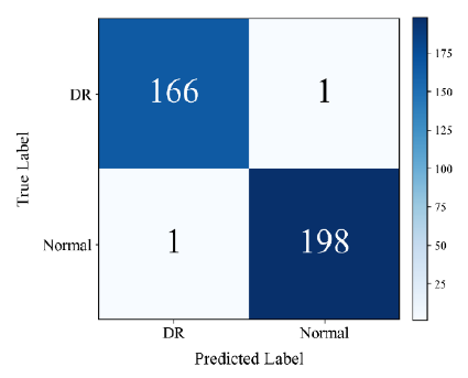
The confusion matrix of the main configuration on the test set is presented in Figure 3.
Figure 3. Confusion matrix of the main configuration (EfficientNet-B1 with random forest importance (RFI)) on the test set (diabetic retinopathy (DR) is the positive class)
As shown in Figure 3, the two misclassifications produced by the main configuration correspond to one false negative (a DR case predicted as Normal) and one false positive (a Normal case predicted as DR).
Given the limited size of the test set (366 images), 95% confidence intervals (CIs) were computed for the accuracy, sensitivity, and specificity of the main configuration. These intervals, obtained using the Wilson score method, are presented in Table 8.
Table 8. Wilson score confidence intervals (CIs) for the main configuration (EfficientNet-B1 with random forest importance (RFI)) on the test set
|
Metric |
Value (%) |
95% CI (%) |
|
Accuracy |
99.45 |
98.03–99.85 |
|
Sensitivity |
99.40 |
96.69–99.89 |
|
Specificity |
99.50 |
97.21–99.91 |
As reported in Table 8, the 95% CIs for the three metrics are relatively wide, particularly at their lower bounds, which is consistent with the limited number of test samples. These intervals quantify the uncertainty of the corresponding point estimates.
The contribution provided by the proposed approach is not limited to classification performance. It also yields a substantially more compact representation. The 1,280-dimensional feature vector obtained from the global average pooling layer of the EfficientNet-B1 architecture was reduced to 94 dimensions (a 92.7% reduction) by means of the RFI method. Similar dimensionality reductions in the range of 91–95% were also obtained for the other CNN architectures (Table 6). This compact representation reduces the input dimensionality and the parameter count of the classifier that operates on the selected features.
3.1.4 Comparison with the literature
In this section, the main configuration of the study (EfficientNet-B1 with RFI; 94 features) is compared with similar studies in the literature on the binary classification of DR. In order to ensure a fair comparison, only studies using the APTOS 2019 dataset were included in the evaluation. The comparative results are presented in Table 9.
Table 9. Comparison of the proposed approach with literature studies performing binary diabetic retinopathy (DR) classification on the Asia Pacific Tele-Ophthalmology Society (APTOS) 2019 dataset
|
Study |
Method |
Accuracy |
|
Rahman et al. [10] |
CLAHE + ResNet-50 + SVM |
96.90% |
|
Butt et al. [11] |
GoogLeNet + ResNet-18 + SVM |
97.80% |
|
Zafar et al. [13] |
Lightweight CNN (1.3 M parameters) |
99.06% |
|
Youldash et al. [8] |
RegNet-X080 |
98.60% |
|
Yang et al. [16] |
ViT + masked self-supervised pretraining |
93.42% |
|
This study |
EfficientNet-B1 + two-stage feature selection (RFI) + ANN |
99.45% |
When Table 9 is examined, it is seen that the proposed approach achieves results competitive with the studies in the literature that use the APTOS 2019 dataset. Among these studies, the highest accuracy was reported by Zafar et al. with their lightweight CNN-based approach at 99.06% [13]. With an accuracy of 99.45% and a 0.9997 AUC, the proposed approach obtains the highest accuracy among the studies included in the comparison.
The main aspect that methodologically distinguishes the proposed approach from the literature is that feature selection methods belonging to four different approaches were systematically evaluated under a single benchmarking framework, and that the high-dimensional deep features were compressed into a compact and discriminative representation. Together, these characteristics allow high classification performance to be achieved on a substantially reduced feature set.
3.2 Discussion
In this section, the results obtained from the experiments are evaluated. Within this scope, the effect of the preprocessing steps on the input images, the deep features of different dimensionalities produced by the four CNN architectures, the comparison of the behaviours of the four feature selection methods, and the effect of the resulting compact feature representations on the classification behaviour are discussed.
Before deep feature extraction, two preprocessing steps, fundus region cropping and CLAHE, are applied to the input images. The cropping step reduces the large, near-zero-valued black background surrounding the fundus and confines the image to the retinal region. In this way, a larger proportion of the spatial resolution is devoted to the retinal tissue rather than to the background. The subsequent CLAHE step, applied only to the L channel in the Lab colour space, enhances local contrast while leaving the A and B channels unchanged. Through this, the intensity histogram is locally redistributed, and the visibility of low-contrast structures such as microaneurysms, small vascular irregularities, and exudates is increased, without removing peripheral retinal tissue or altering the colour composition of the lesions.
The deep feature vectors produced by the four architectures differ considerably in size, ranging from 768 dimensions for ConvNeXt-Tiny to 2,048 for ResNet-50. This size is set by the width of each network’s final stage, which is a property of the architecture design rather than of the fundus images. In the fine-tuning-only results in Table 4, the larger 2,048-dimensional representation of ResNet-50 did not achieve higher accuracy than the 1,280-dimensional representation of EfficientNet-B1. This shows that a higher dimensionality does not by itself provide a more discriminative representation.
Among the four different feature selection methods applied in the proposed approach, the RFI method both produced consistent compact representations within a narrow range and achieved high accuracy across all CNN architectures. One of the main reasons for this is that the Random Forest algorithm can effectively capture the nonlinear interactions and rank-level relationships among features. Since deep features are inherently high-dimensional and have complex relationships, tree-based importance measures offer a reduction strategy compatible with such features. In addition, the RFI method provides a more flexible threshold mechanism (above the mean importance) compared with Boruta’s statistical confirmation mechanism. Moreover, this method is free from dependence on the adaptive cutoff in mRMR and the sensitivity to the regularization coefficient selection in Lasso. When these characteristics are evaluated together, it is seen that the RFI method is a suitable and effective choice for deep feature-based classification.
Although the other three feature selection methods also provided meaningful improvements over the fine-tuning-only performances, they showed some differences from the RFI method in terms of compactness and overall stability. The number of features retained by each method follows from its selection principle. Although the Boruta method has a theoretically strong infrastructure thanks to shadow feature comparison and the statistical confirmation mechanism, it produced a relatively large subset, such as 387 features on the ResNet-50 architecture, and therefore met the dimensionality reduction goal to a more limited extent. The mRMR method showed a wide range of feature counts between 20 and 200 depending on the value of the adaptive cutoff. In particular, it dropped to 98.63% accuracy with 20 features on the ResNet-50 architecture, revealing that overly aggressive reduction can adversely affect performance. While the Lasso method produced some of the most compact representations (36 features for EfficientNet-B1), the number of features it selected varied over a wide range across the architectures, from 36 to 122. These findings emphasize the importance of choosing a method compatible with the deep feature distribution rather than applying the feature selection method uniformly.
The compression of the deep features into a compact subset also affects the classification behaviour. As shown in Table 6, although this reduction removed a large part of the features, the accuracy across the four architectures was maintained and even slightly increased relative to the fine-tuning-only models. This indicates that the deep feature space contains substantial redundancy for the binary task, and that a compact subset can retain the information needed to distinguish the two classes. In addition, by removing low-variance and redundant features, feature selection can reduce the risk of overfitting.
When evaluated overall, the proposed approach offers a binary DR classification solution that can effectively leverage the deep representation power of modern CNN architectures on a compact, selected feature subset. This solution also exhibits consistent performance across the different CNN architectures. The 99.45% accuracy and 0.9997 AUC obtained on the 94-dimensional representation formed by the EfficientNet-B1 architecture together with the RFI method reveal that the proposed method achieves performance competitive with common approaches in the literature.
In this study, feature selection methods from different approaches were systematically compared on deep features for the binary classification of DR from fundus images, using the APTOS 2019 dataset. The main configuration, obtained by combining EfficientNet-B1 with RFI, reduced the feature dimensionality from 1,280 to 94 and reached 99.45% accuracy and a 0.9997 AUC, improving on the fine-tuning-only models and achieving results competitive with those reported in the literature. These results indicate that applying feature selection to deep features can yield compact yet high-performing representations for binary DR classification. Nevertheless, the use of a single competition dataset without external validation and the binary classification of DR (DR/Normal) constitute important limitations regarding the generalizability of the model. In addition, since the classification performance was evaluated only through the numerical values on the test subset, the performance of the model under real clinical deployment conditions cannot be precisely predicted. In future studies, additional experiments are planned on multi-center and external validation datasets covering different camera types, patient populations, and labeling protocols (such as IDRiD, Messidor-2, and EyePACS). Furthermore, the adaptation of the proposed approach to the multi-class grading of DR severity is also planned.
In terms of model development, future studies aim to integrate transformer-based components, self-attention mechanisms, and graph neural networks that can more effectively model the long-range dependencies in fundus images. It is anticipated that such hybrid structures, by combining the complementary strengths of CNN-based local feature extraction and transformer-based global context modeling, could strengthen the generalizability and robustness of the model, particularly on multi-center and external datasets, and could contribute to more challenging tasks such as the multi-class grading of DR severity. Explainability approaches that visualize the model's decision processes and quantify prediction uncertainty are planned to be added to the proposed approach. Within this scope, explainable artificial intelligence techniques such as Gradient-weighted Class Activation Mapping (Grad-CAM), feature importance visualizations, and uncertainty estimation methods will be integrated into the proposed approach. Furthermore, subject to successful multi-center and external validation, the evaluation of the system in real clinical environments could be addressed at a later stage.
This research received no specific grant from any funding agency in the public, commercial, or not-for-profit sectors. The source code and trained model weights developed within this study will be made available by the corresponding author upon reasonable request.
|
ANN |
artificial neural network |
|
APTOS |
Asia Pacific Tele-Ophthalmology Society |
|
AUC |
area under the curve |
|
BN |
batch normalization |
|
CI |
confidence interval |
|
CLAHE |
contrast limited adaptive histogram equalization |
|
CNN |
convolutional neural network |
|
CUDA |
Compute Unified Device Architecture |
|
DR |
diabetic retinopathy |
|
FN |
false negative |
|
FP |
false positive |
|
GPU |
graphics processing unit |
|
Grad-CAM |
Gradient-weighted Class Activation Mapping |
|
IDRiD |
Indian Diabetic Retinopathy Image Dataset |
|
K |
dimension of the compact feature vector (dimensionless) |
|
Lab |
CIELAB color space |
|
mRMR |
minimum redundancy maximum relevance |
|
ReLU |
rectified linear unit |
|
RFI |
random forest importance |
|
RGB |
red–green–blue |
|
RLROP |
ReduceLROnPlateau |
|
ROC |
receiver operating characteristic |
|
SVM |
support vector machine |
|
TN |
true negative |
|
TP |
true positive |
|
ViT |
vision transformer |
[1] Morya, A.K., Ramesh, P.V., Nishant, P., et al. (2024). Diabetic retinopathy: A review on its pathophysiology and novel treatment modalities. World Journal of Methodology, 14(4): 95881. https://doi.org/10.5662/wjm.v14.i4.95881
[2] Wang, Z., Zhang, N., Lin, P., Xing, Y., Yang, N. (2024). Recent advances in the treatment and delivery system of diabetic retinopathy. Frontiers in Endocrinology, 15: 1347864. https://doi.org/10.3389/fendo.2024.1347864
[3] Teo, Z.L., Tham, Y.C., Yu, M., et al. (2021). Global prevalence of diabetic retinopathy and projection of burden through 2045. Ophthalmology, 128(11): 1580-1591. https://doi.org/10.1016/j.ophtha.2021.04.027
[4] Kąpa, M., Koryciarz, I., Kustosik, N., Jurowski, P., Pniakowska, Z. (2024). Modern approach to diabetic retinopathy diagnostics. Diagnostics, 14(17): 1846. https://doi.org/10.3390/diagnostics14171846
[5] Umamageswari, A., Anita, C.S., Beevi, L.S., Sangari, A. (2025). Deep learning based object detection in medical image with YOLOv4-CSP with U-Net algorithms. Traitement du Signal, 42(1): 167-176. https://doi.org/10.18280/ts.420115
[6] Mienye, I.D., Swart, T.G., Obaido, G., Jordan, M., Ilono, P. (2025). Deep convolutional neural networks in medical image analysis: A review. Information, 16(3): 195. https://doi.org/10.3390/info16030195
[7] Saproo, D., Mahajan, A.N., Narwal, S. (2024). Deep learning based binary classification of diabetic retinopathy images using transfer learning approach. Journal of Diabetes & Metabolic Disorders, 23(2): 2289-2314. https://doi.org/10.1007/s40200-024-01497-1
[8] Youldash, M., Rahman, A., Alsayed, M., et al. (2024). Early detection and classification of diabetic retinopathy: A deep learning approach. AI, 5(4): 2586-2617. https://doi.org/10.3390/ai5040125
[9] Anand, V., Koundal, D., Alghamdi, W.Y., Alsharbi, B.M. (2024). Smart grading of diabetic retinopathy: An intelligent recommendation-based fine-tuned EfficientNetB0 framework. Frontiers in Artificial Intelligence, 7: 1396160. https://doi.org/10.3389/frai.2024.1396160
[10] Rahman, A., Youldash, M., Alshammari, G., et al. (2024). Diabetic retinopathy detection: A hybrid intelligent approach. Computers, Materials & Continua, 80(3): 4561-4576. https://doi.org/10.32604/cmc.2024.055106
[11] Butt, M.M., Iskandar, D.N.F.A., Abdelhamid, S.E., Latif, G., Alghazo, R. (2022). Diabetic retinopathy detection from fundus images of the eye using hybrid deep learning features. Diagnostics, 12(7): 1607. https://doi.org/10.3390/diagnostics12071607
[12] Sapra, V., Sapra, L., Bhardwaj, A., Almogren, A., Bharany, S., Rehman, A.U., Ouahada, K. (2024). Diabetic retinopathy detection using deep learning with optimized feature selection. Traitement du Signal, 41(2): 781-790. https://doi.org/10.18280/ts.410219
[13] Zafar, A., Kim, K.S., Ali, M.U., Byun, J.H., Kim, S.H. (2025). A lightweight multi-deep learning framework for accurate diabetic retinopathy detection and multi-level severity identification. Frontiers in Medicine, 12: 1551315. https://doi.org/10.3389/fmed.2025.1551315
[14] Liu, C., Wang, W., Lian, J., Jiao, W. (2025). Lesion classification and diabetic retinopathy grading by integrating softmax and pooling operators into vision transformer. Frontiers in Public Health, 12: 1442114. https://doi.org/10.3389/fpubh.2024.1442114
[15] Shakibania, H., Raoufi, S., Pourafkham, B., Khotanlou, H., Mansoorizadeh, M. (2024). Dual branch deep learning network for detection and stage grading of diabetic retinopathy. Biomedical Signal Processing and Control, 93: 106168. https://doi.org/10.1016/j.bspc.2024.106168
[16] Yang, Y., Cai, Z., Qiu, S., Xu, P. (2024). Vision transformer with masked autoencoders for referable diabetic retinopathy classification based on large-size retina image. PLoS ONE, 19(3): e0299265. https://doi.org/10.1371/journal.pone.0299265
[17] Yu, C., Ma, Q., Li, J., et al. (2025). FF-ResNet-DR model: A deep learning model for diabetic retinopathy grading by frequency domain attention. Electronic Research Archive, 33(2): 725-743. https://doi.org/10.3934/era.2025033
[18] Bajwa, A., Nosheen, N., Talpur, K.I., Akram, S. (2023). A prospective study on diabetic retinopathy detection based on modify convolutional neural network using fundus images at Sindh Institute of Ophthalmology & Visual Sciences. Diagnostics, 13(3): 393. https://doi.org/10.3390/diagnostics13030393
[19] Asia Pacific Tele-Ophthalmology Society. (2019). APTOS 2019 blindness detection. Kaggle. https://www.kaggle.com/competitions/aptos2019-blindness-detection.
[20] MariaHerreroT. (2021). APTOS-2019 dataset. Kaggle. https://www.kaggle.com/datasets/mariaherrerot/aptos2019.
[21] Hemamalini, S., Kumar, V.D.A., Ramachandran, V., Robin, R. (2024). Retinal image enhancement through hyperparameter selection using RSO for CLAHE to classify diabetic retinopathy. Traitement du Signal, 41(4): 2003-2012. https://doi.org/10.18280/ts.410429
[22] Buslaev, A., Iglovikov, V.I., Khvedchenya, E., Parinov, A., Druzhinin, M., Kalinin, A.A. (2020). Albumentations: Fast and flexible image augmentations. Information, 11(2): 125. https://doi.org/10.3390/info11020125
[23] Tan, M.X., Le, Q.V. (2019). EfficientNet: Rethinking model scaling for convolutional neural networks. In International Conference on Machine Learning, Long Beach, CA, USA, pp. 6105-6114. https://doi.org/10.48550/arXiv.1905.11946
[24] Huang, G., Liu, Z., Van Der Maaten, L., Weinberger, K.Q. (2017). Densely connected convolutional networks. In 2017 IEEE Conference on Computer Vision and Pattern Recognition (CVPR), Honolulu, HI, USA, pp. 2261-2269. https://doi.org/10.1109/cvpr.2017.243
[25] He, K., Zhang, X., Ren, S., Sun, J. (2016). Deep residual learning for image recognition. In 2016 IEEE Conference on Computer Vision and Pattern Recognition (CVPR), Las Vegas, NV, USA, pp. 770-778. https://doi.org/10.1109/cvpr.2016.90
[26] Liu, Z., Mao, H., Wu, C.Y., Feichtenhofer, C., Darrell, T., Xie, S. (2022). A ConvNet for the 2020s. In 2022 IEEE/CVF Conference on Computer Vision and Pattern Recognition (CVPR), New Orleans, LA, USA, pp. 11966-11976. https://doi.org/10.1109/cvpr52688.2022.01167
[27] Russakovsky, O., Deng, J., Su, H., et al. (2015). ImageNet large scale visual recognition challenge. International Journal of Computer Vision, 115(3): 211-252. https://doi.org/10.1007/s11263-015-0816-y
[28] Kursa, M.B., Rudnicki, W.R. (2010). Feature selection with the Boruta package. Journal of Statistical Software, 36(11): 1-13. https://doi.org/10.18637/jss.v036.i11
[29] Manikandan, G., Pragadeesh, B., Manojkumar, V., Karthikeyan, A.L., Manikandan, R., Gandomi, A.H. (2024). Classification models combined with Boruta feature selection for heart disease prediction. Informatics in Medicine Unlocked, 44: 101442. https://doi.org/10.1016/j.imu.2023.101442
[30] Peng, H., Long, F., Ding, C. (2005). Feature selection based on mutual information criteria of max-dependency, max-relevance, and min-redundancy. IEEE Transactions on Pattern Analysis and Machine Intelligence, 27(8): 1226-1238. https://doi.org/10.1109/tpami.2005.159
[31] Ihianle, I.K., Machado, P., Owa, K., Adama, D.A., Otuka, R., Lotfi, A. (2024). Minimising redundancy, maximising relevance: HRV feature selection for stress classification. Expert Systems with Applications, 239: 122490. https://doi.org/10.1016/j.eswa.2023.122490
[32] Tibshirani, R. (1996). Regression shrinkage and selection via the lasso. Journal of the Royal Statistical Society Series B: Statistical Methodology, 58(1): 267-288. https://doi.org/10.1111/j.2517-6161.1996.tb02080.x
[33] Li, Y., Gao, X., Tang, X., Lin, S., Pang, H. (2023). Research on automatic classification technology of kidney tumor and normal kidney tissue based on computed tomography radiomics. Frontiers in Oncology, 13: 1013085. https://doi.org/10.3389/fonc.2023.1013085
[34] Breiman, L. (2001). Random forests. Machine Learning, 45(1): 5-32. https://doi.org/10.1023/a:1010933404324
[35] Wang, X., Zhou, Q., Li, H., Chen, M. (2023). Enhancing feature selection for imbalanced Alzheimer’s disease brain MRI images by random forest. Applied Sciences, 13(12): 7253. https://doi.org/10.3390/app13127253
[36] Kingma, D.P., Ba, J. (2014). Adam: A method for stochastic optimization. arXiv preprint arXiv:1412.6980. https://doi.org/10.48550/arXiv.1412.6980