Prabhu Teja Geddada* | Rajesh Kumar Pullagura
© 2026 The authors. This article is published by IIETA and is licensed under the CC BY 4.0 license (http://creativecommons.org/licenses/by/4.0/).
OPEN ACCESS
Keratoconus is a progressive corneal disorder characterized by corneal thinning and irregular deformation, which may lead to visual impairment if not identified at an early stage. This study proposes an automated multiclass classification framework for keratoconus assessment using Pentacam-based corneal topographic maps. The proposed framework integrates discrete wavelet transform (DWT)-based feature extraction, L1-regularized logistic regression for feature selection, and a Light Gradient Boosting Machine (LightGBM) classifier. Multiple wavelet families, including biorthogonal, Coiflet, Daubechies, and reverse biorthogonal wavelets, were investigated to identify effective frequency-domain representations of corneal characteristics. The selected features were used to classify three categories: keratoconus, normal, and suspect cases. The performance of LightGBM was compared with Support Vector Machine (SVM), Random Forest (RF), and eXtreme Gradient Boosting (XGBoost) classifiers using accuracy, macro-F1 score, and macro-averaged area under the receiver operating characteristic curve (macro-AUC). Experimental results showed that the Coiflet-3 wavelet combined with LightGBM achieved the best overall performance, obtaining an accuracy of 87.76%, a macro-F1 score of 0.8727, and a macro-AUC of 0.9580. Additional analysis demonstrated that the proposed approach effectively captures discriminative frequency-domain features from corneal topographic maps while maintaining model interpretability through feature selection. These findings indicate that the proposed framework can provide a reliable computer-aided approach for supporting keratoconus screening and clinical decision-making.
keratoconus, Pentacam corneal topograph, discrete wavelet transform, Light Gradient Boosting Machine, machine learning, multiclass classification
Keratoconus is an eye disease that results in gradual thinning of the cornea, leading to reduced vision [1]. Traditionally described as non-inflammatory [2], recent studies show that eyes with keratoconus have some form of inflammation [3]. Although keratoconus is a bilateral disorder, one eye tends to be affected more severely than the other [4]. The disease typically manifests after puberty and progresses at a varied rate over two to three decades [5]. Advanced cases of keratoconus can be readily identified due to the presence of clinical symptoms such as Munson’s sign, Fleischer’s Ring, Rizzuti’s sign, and Vogt’s striae [6]. Ophthalmologists diagnose this disease based on corneal topography and tomography. These instruments provide detailed information about corneal curvature [7]. Early intervention for keratoconus is vital, as the disease progression can be slowed through corneal collagen cross-linking [8]. However, early diagnosis can be difficult because the disease may not present noticeable symptoms in its initial stages [9]. Moreover, the diagnostic grading of subclinical keratoconus has not reached a global consensus [10], unlike that of diabetic retinopathy [11].
To address these issues, many machine learning models have been proposed to aid ophthalmologists in detecting keratoconus. Machine learning and deep learning (DL) may improve diagnostic accuracy and reduce the burden on healthcare personnel when implemented as an automated screening tool [12].
The main aim of this study is to evaluate the classification performance of machine learning in detecting keratoconus from corneal topographic maps obtained from the Pentacam High Resolution (HR) instrument. Although automated classification methods have progressed, the overall performance remains limited due to fundamental challenges such as feature subtlety and class imbalance, particularly for suspect cases whose topographic patterns can closely resemble those of normal corneas. Moreover, the suspect samples are generally underrepresented compared to normal and keratoconus cases, introducing additional difficulty during model training.
The proposed methodology employs discrete wavelet transform (DWT)-based feature extraction within the L*a*b* color space for keratoconus classification. Feature selection was performed using logistic regression with L1 regularization to enhance model interpretability by isolating the most discriminative wavelet coefficients, thereby reducing feature dimensionality. The final classification was performed using a hyperparameter-optimized Light Gradient Boosting Machine (LightGBM) classifier.
The remainder of this paper is organized as follows: Section 2 reviews the related work on keratoconus detection and wavelet-based image analysis in medical imaging. Section 3 describes the complete methodological pipeline, including data acquisition, preprocessing, DWT-based feature extraction from the L*a*b* color space, feature selection, and the LightGBM classification framework. Section 4 presents the performance metrics, evaluation results, and experimental setup, followed by a comprehensive discussion in Section 5. Finally, Section 6 concludes the paper with key findings and future research directions.
In scientific literature, there are numerous papers that employ machine learning algorithms in keratoconus detection [13]. Ali et al. [14] used a supervised machine learning approach to detect keratoconus from a sample size of 40 cases derived from corneal topographic maps. They employed image processing and geometric techniques to extract 12 features from topographic maps. The features were fed to a Support Vector Machine (SVM) classifier to classify between healthy and keratoconus eyes. Their method achieved an accuracy of 90% on a test set of 10 cases. Yousefi et al. [15] proposed an unsupervised machine learning model for keratoconus severity identification. They used 420 corneal parameters derived from 3156 eyes using CASIA OCT imaging systems. Their approach employed Principal Component Analysis (PCA) to reduce the dimensionality of corneal parameters from 420 to eight and t-distributed stochastic neighbor embedding (t-SNE) to further reduce the eight principal components to two eigen-parameters. A density-based clustering algorithm was applied in the 2D t-SNE space to group eyes with similar corneal characteristics into non-overlapping clusters.
Lavric et al. [16] utilized 443 corneal parameters from 3151 samples corresponding to 3146 eyes for keratoconus detection. To select the corneal parameters with the most discriminative capability in detecting the disease, subset selection and feature ranking were used. Using these feature selection approaches, the eight best parameters were selected and were used to train 25 machine learning models with 10-fold cross-validation. Out of 25 models, SVM obtained the highest classification accuracy of 94% for binary classification between healthy and keratoconus eyes and 93% accuracy for multi-class classification between healthy, forme fruste, and keratoconic eyes. Al-Sharify et al. [17] considered 491 cases to analyze the effect of keratoconus. They used seven corneal parameters to train two models, decision trees and nearest neighbor analysis (NNA), for keratoconus identification. Five pathological conditions, keratoconus, normal, subclinical, forme fruste keratoconus, and ectasia, were considered. The proposed model achieved an accuracy of 65.7% with decision trees and 62.6% with NNA.
An early keratoconus screening framework proposed by Chaari et al. [18] integrated an automated feature selection of corneal parameters using select K-best with analysis of variance (ANOVA). Out of 443 corneal parameters from 3162 patients, the 50 best features were selected to train 3 machine learning models: SVM, K-Nearest Neighbour (KNN), and Artificial Neural Networks (ANNs) with 5-fold cross-validation. Using the best 50 features, SVM performed better for two-class classification with an accuracy of 97.08%, and ANN achieved the highest accuracy for the 4-class problem with 94.78%. It should be noted that without feature selection, the study reported an accuracy of 98.95% for the 2-class problem and 96% for the 4-class problem with the SVM classifier. In contrast, the study [14] reported a test accuracy of 90% on a test set of 10 cases, which limits the reliability of model’s performance. Although the studies [15, 16] have shown reliable performance, they considered the CASIA ESI index as the ground truth rather than the clinical diagnosis labels while reporting their model’s performance.
In their study, Kuo et al. [19] presented a DL framework to screen keratoconus from corneal topographic maps. Their work included 354 corneal topographic images consisting of 170 keratoconus images, 28 subclinical keratoconus images, and 156 normal topographic maps. Three DL models were trained, namely VGG16, Inception V3, and ResNet152. The accuracy of VGG16 and Inception V3 was 0.931, and that of ResNet152 was 0.958. The model’s reported accuracies were those of a two-class problem between keratoconus and normal eyes. The authors used the entire subclinical images as a separate subclinical test set to assess the model’s ability to predict subclinical cases. The accuracy of their model when subclinical cases were used as test set was around 28.5% to 39.2%. Al-Timemy et al. [20] developed 7 DL models using EfficientNet-B0 and extracted 1000 deep features from each corneal map type to form 7000 features. These features were used to train an SVM classifier to classify the disease. The proposed hybrid DL model achieved an accuracy of 81.5% on a development dataset of 542 eyes. It achieved 68.7% accuracy on an independent dataset of 150 eyes, and 84.4% accuracy on the merged dataset consisting of 692 eyes for a 3-class problem. For the two-class problem, they achieved accuracies of 98.5%, 92%, and 97.7% on datasets of 542 eyes, 150, and 692 eyes, respectively.
Kallel et al. [21] used 60 topographic maps along with image generator models, namely SyntEyes and Generative Adversarial Network (GAN) models, to train seven different DL models. Their study reported an accuracy ranging from 95.31% to 99.74% and recall between 98.71% and 95.74% for a two-class problem. Gandhi et al. [22] trained eight DL models on 372 corneal topographic maps to classify the disease as per the Amsler–Krumeich standard. Their approach included converting the input images with edges and color masks to grayscale and applying Law’s texture method to derive an edge map. These edge maps were fed to DL models. Out of the seven models trained, VGG19 achieved better training and testing accuracies of 99.62% and 77.43%, respectively. Ahmed et al. [23] used 4011 corneal topographic maps consisting of three classes, namely keratoconus, normal, and suspect, for 3-class classification of the disease. Data augmentation was applied to increase the sample size to 16,016 samples. The entire dataset was split into training, validation, and test sets with an 80-10-10 split. Eight DL models were trained to test classification performance. Their results showed that MobileNetV2 outperformed the rest of the models with 98% accuracy on the test set. While this arXiv preprint study reported near-perfect detection of the disease, the performance can be attributed to reliance on heavy data augmentation. The model developed in the study [19], although it achieved better performance in a two-class problem, failed to detect subclinical cases. The study [21] relied heavily on GAN/SyntEyes models while reporting their model’s performance. The study [22] reported high training accuracy with poor test accuracy, suggesting that their model might be overfitting.
Recent advances in DL extended keratoconus detection beyond conventional CNN architectures. Lu et al. [24] introduced the Corneal Multiview Fusion Transformer (CMVFT), which combines features from seven standard corneal topography maps using pretrained ResNet-50, a multi-scale attention module, and a fusion transformer for keratoconus classification. Although the model showed promise in identifying suspect cases, its architectural complexity and dependence on multi-view inputs may hinder routine clinical deployment. Abdelmotaal et al. [25] proposed a hybrid CNN-transformer framework that analyses Scheimpflug-based dynamic corneal deformation videos using transfer learning and attention mechanisms. It achieved an area under the curve (AUC) of 0.97 and a sensitivity of 93%. However, the method requires Corvis-generated dynamic videos, making it unsuitable for conventional Pentacam-based screening.
Sujitha et al. [26] developed a framework integrating an improved Swin Transformer block with residual Multi-Layer Perceptrons (MLP), optimized through the Polar Fox metaheuristic algorithm and SHapley Additive exPlanations (SHAP)-based explainability. The method reported an accuracy of 99.4% on a benchmark dataset. However, such results are generally obtained under binary classification and may not generalize to imbalanced three-class clinical datasets. Kandakji et al. [27] employed principal component analysis followed by Gaussian Mixture modelling on a large AS-OCT dataset comprising 25,816 corneal scans from 5,005 patients. Their semi-supervised framework identified a distinct subclinical keratoconus subgroup with a higher likelihood of progressing to clinical keratoconus. Despite its value for early risk stratification, the approach relies on extracted corneal indices rather than raw topographic images and was not validated for Pentacam image classification.
Jawad et al. [28] utilized Red, Green, and Blue (RGB) to L*a*b* color space conversion and applied Contrast Limited Adaptive Histogram Equalization (CLAHE) on the L-channel to enhance the retinal image quality, thereby improving disease identification. Harikumar et al. [29] proposed DWT for feature extraction from MRI images for classification of medical images between normal and pathological cases. They employed Haar, Daubechies, Biorthogonal, and Coiflet wavelets to extract features and train four neural networks. They achieved better classification accuracy with the RBF network and the db4 wavelet. Ryali and Menon [30] used logistic regression with L1 norm regularization for feature selection and classification of fMRI data.
Overall, these studies demonstrate the effectiveness of advanced deep learning (DL) and ensemble techniques, yet several limitations remain. Transformer-based methods often require substantial computational resources on specialized imaging modalities, while ensemble approaches based on handcrafted clinical indices are not readily transferable to raw image classification. Furthermore, no earlier studies investigated the contribution of individual wavelet subbands and color channels to keratoconus classification, leaving the interpretability of frequency-domain features unexplored.
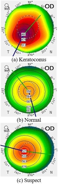
In the corneal topographic maps, the corneal irregularities are represented by warm colors, and normal patterns are represented by cool colors. We hypothesize that using the color-coded information of the corneal maps and decomposing the color channels into multiple sub-bands using 2D-DWT can extract high-frequency spatial texture that can capture subtle changes in the cornea. These multi-scale features, when used as inputs to a machine learning classifier, can improve the classification accuracy.
3.1 Data collection
In this study, 2961 corneal images gathered from 423 eyes using Oculus Pentacam were included. This dataset was made available to the research community through earlier studies [20]. The dataset consists of three classes: (1) keratoconus, (2) normal, (3) suspect. It was labelled as such by three corneal specialists based on standard criteria in earlier studies [20].
The keratoconus and normal classes have 150 eyes with seven maps per eye. The suspect class has 123 eyes with seven maps per eye. All images have the size of 224 × 224 × 3 and were acquired using the Oculus Pentacam HR instrument. As this study utilized a previously published, de-identified dataset [20], independent ethical approval was not required. Ethical clearance for data collection and labelling was obtained in the originating study. Patient demographic details, inclusion and exclusion criteria, and data acquisition protocols were reported in the study [20] and were not collected in this study. Figure 1 shows the corneal topographic maps: (a) keratoconus, (b) normal, and (c) suspect.
3.2 Data preprocessing
The entire dataset was split into a 70% training set, a 15% validation set, and a 15% test set. The training set contains 297 eyes with 2079 images, the validation set contains 63 eyes with 441 images, and the test set contains 63 eyes with 441 images. The split was performed at the eye level to prevent data leakage, as all 7 maps from a single eye share correlated topographic information. Since the dataset is imbalanced, class weighting was applied to assign larger weights to underrepresented classes during training. The class weights were computed using the balanced weighting approach.
$w_j=\frac{N_{\text {train }}}{K \times N_j}$ (1)
where,
$w_j$ is the weight for class j,
$N_{\text {train}}$ is the total number of samples in the training set,
K is the total number of target classes,
$N_j$ represents the total number of samples corresponding to class j within the training data.
In addition to class weighting, to address class imbalance, the Synthetic Minority Over-Sampling Technique (SMOTE) [31] was applied as an alternative balancing strategy for comparative analysis. SMOTE was applied exclusively on the training data to avoid information leakage into validation or test sets. The implementation used the default SMOTE configuration with k_neighbors = 5 and random_state = 42. Synthetic minority samples were generated in the selected feature space after feature scaling and selection.
Before feature extraction, all RGB corneal maps were converted into the L*a*b* color space. It provides perceptual color separation and has been used to improve medical image analysis performance [28].
In this work, it is used as a preprocessing step before feature extraction. The images are converted from the RGB color space to the L*a*b* color space using the following transformations shown in Eqs. (2) to (6).
$\left[\begin{array}{l}X \\ Y \\ Z\end{array}\right]=\left[\begin{array}{lll}0.41 & 0.35 & 0.18 \\ 0.21 & 0.71 & 0.07 \\ 0.01 & 0.11 & 0.95\end{array}\right]\left[\begin{array}{l}R^{\prime} \\ G^{\prime} \\ B^{\prime}\end{array}\right]$ (2)
$f(r)=\left\{\begin{array}{cc}r^{1 / 3} & r>e \\ 7.787 r+\frac{16}{116} & r \leq e\end{array}\right.$ (3)
$L^*=\left\{\begin{array}{l} 116\left(\frac{Y}{Y_n}\right)^{1 / 3}-16 \frac{Y}{Y_n}>e \\ 903.3\left(\frac{Y}{Y_n}\right) \quad \frac{Y}{Y_n} \leq e \end{array} \quad \text { where, } e=0.008856\right.$ (4)
$a^*=500\left(f\left(\frac{X}{X_n}\right)-f\left(\frac{Y}{Y_n}\right)\right)$ (5)
$b^*=200\left(f\left(\frac{Y}{Y_n}\right)-f\left(\frac{Z}{Z_n}\right)\right)$ (6)
No pixel-level normalization is applied to raw images; standardization is performed on the extracted wavelet feature vectors using StandardScaler, fitted on the training set and applied to validation and test sets.
Figure 1. Corneal topography images
3.3 Extraction of features using wavelets
After L*a*b* conversion, DWT is applied to extract multi-scale texture and frequency features from corneal maps. Unlike the Fourier transform, wavelet transforms preserve both frequency and spatial localization. In this study, several wavelet families were evaluated, including Biorthogonal (bior1.5, bior2.2, bior3.3), Coiflets (coif2, coif3), Daubechies (db4, db5, db6). Haar, Reverse Biorthogonal (rbio2.2, rbio3.1, rbio3.3), and Symlets (sym4, sym6) were also evaluated. Haar wavelets are simple and effective for edge detection whereas Daubechies provide compactness and strong spatial frequency localization. Biorthogonal and Reverse Biorthogonal were employed for their symmetric reconstruction. Symlets and Coiflets were included for their near-symmetry and vanishing moments. The final selected wavelets, bior1.5, coif3, db6, and rbio2.2, were chosen based on their discriminative capability, reconstruction characteristics, and classification performance during initial experimental evaluation. The decomposition level for all the wavelets was set to 4.
3.4 Feature selection using L1 logistic regression
Feature selection was performed to reduce dimensionality, remove redundant features, and improve classification performance. In this study, Logistic Regression with L1 regularization was chosen for feature selection because it effectively removes irrelevant features while preserving discriminative information [30]. L1 regularization forces less informative feature coefficients toward zero, resulting in a sparse optimized feature subset.
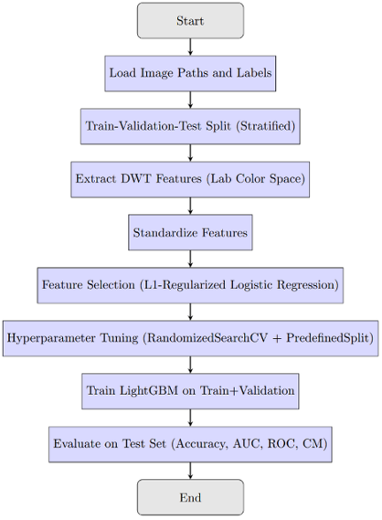
The solver for logistic regression was set to ‘liblinear’ with maximum iterations of ‘10,000’, and the parameter ‘C’ was set to its default value of 1.0. Features with non-zero coefficients after model fitting were retained for further analysis, while those with zero coefficients were discarded. Figure 2 shows the proposed workflow for keratoconus detection.
Figure 2. Workflow for wavelet-based keratoconus detection with Light Gradient Boosting Machine (LightGBM) classifier
3.5 Light Gradient Boosting Machine
LightGBM [32] is a gradient boosting framework designed for efficient and scalable machine learning. It improves computational efficiency using histogram-based learning and leaf-wise growth.
In this study, LightGBM was trained on wavelet-based features extracted from corneal topographic maps. While traditional classifiers such as SVM and Random Forest (RF) are robust, LightGBM was selected because its leaf-wise tree growth strategy provides computationally efficient handling of high-dimensional feature sets commonly encountered in medical imaging.
To empirically validate the classifier choice, four candidate classifiers, namely SVM with Radial Basis Function (RBF) kernel, RF, eXtreme Gradient Boosting (XGBoost) were evaluated on identical L1-selected DWT features.
RandomizedSearchCV was used to optimize the classifier hyperparameters. Thirty randomly selected hyperparameter combinations were evaluated using a PredefinedSplit strategy, with a fixed validation set serving as the hold-out fold for model selection.
Under this setup, the model was trained on the primary training set, and hyperparameters were optimized based on a single, fixed validation subset of 63 eyes (441 samples). The best hyperparameter combination was selected based on the performance achieved on the validation subset. The validation set served as the definitive hold-out fold to determine the best hyperparameter combination before final testing.
Table 1 shows the candidate classifiers, their tunable parameters and the corresponding search ranges.
Following model training, a subband-wise feature importance analysis was performed to determine the frequency domain components most relevant to classification. Feature importance scores obtained from LightGBM were grouped according to subband type (LL, LH, HL, HH), decomposition stages (levels 1–4), and L*a*b* color channel.
Table 1. Hyperparameter search space for Light Gradient Boosting Machine (LightGBM) classifier
|
Classifier |
Parameter |
Search Space |
|
SVM (RBF) |
C, gamma |
[0.1,1000] {scale, auto} |
|
Random Forest |
n_estimators, max_depth, min_samples_split, min_samples_leaf, max_features |
[100,600], [3,20], [2,12], [1,8], {sqrt, log2, None} |
|
XGBoost |
n_estimators, max_depth, learning_rate, subsample, colsample_bytree |
[50,500], [3,10], [0.01,0.20], [0.5,1.0], [0.5,1.0] |
|
LightGBM |
num_leaves, max_depth, learning_rate, n_estimators, subsample, colsample_bytree |
[20,150], [3,10], [0.01,0.20], [50,500], [0.5,1.0], [0.5,1.0] |
To account for variability, bootstrapping with 1000 resamples was applied. For each iteration, a bootstrap sample was drawn from the test set with replacement, and the metrics were recomputed without retraining the model. The metrics from the 1000 iterations were used to estimate 95% confidence interval (CI).
A one-way ANOVA was then applied to determine whether the selected wavelets significantly differed in average performance. When a significant effect was observed, Tukey’s HSD test was used to perform pairwise comparisons among the pipelines. In addition, t-tests were conducted on the bootstrap-generated samples to examine the performance difference between the class weighting approach and SMOTE-based balancing techniques. These evaluation methods are commonly employed to assess comparative model performance [33].
The search ranges for hyperparameters in Table 1 were chosen to ensure a balance between model complexity and the risk of overfitting.
The multi-class classification performance of the LightGBM classifier was evaluated on the test subset of 63 eyes (441 samples). The evaluation metrics include accuracy, sensitivity (recall), specificity, precision, F1-score, AUC score and receiver operating characteristic (ROC) curves. ROC is a graphical representation of a classifier’s ability, with False Positive Rate (FPR) and True Positive Rate (TPR) on the x- and y-axes, respectively.
While precision evaluates the reliability of abnormal predictions, recall measures the ability to correctly identify the diseased cases. F1-score provides a balanced evaluation of precision and recall, and AUC evaluates the classifier’s ability to distinguish between classes across different decision thresholds. In addition, both macro-average and weighted-average metrics were reported to evaluate the model’s performance under class imbalance conditions. Macro-average metrics assign equal importance to all classes, including the minority class, and weighted-average metrics account for class distribution and provide an overall performance estimate.
Table 2 shows the optimized LightGBM parameters corresponding to each discrete wavelet family used for feature extraction. These values were obtained through hyperparameter optimization using the randomized search technique.
Table 2. Best hyperparameter settings for each wavelet family using the class-weighting method
|
Hyperparameter |
bior1.5 |
coif3 |
db6 |
rbio2.2 |
|
num_leaves |
34 |
57 |
33 |
143 |
|
max_depth |
6 |
6 |
4 |
4 |
|
learning_rate |
0.0379 |
0.2039 |
0.2039 |
0.1179 |
|
n_estimators |
237 |
463 |
93 |
266 |
|
subsample |
0.7280 |
0.5003 |
0.8636 |
0.6379 |
|
colsample_bytree |
0.8059 |
0.5102 |
0.5924 |
0.8736 |
$\text { Accuracy }=\frac{T P+T N}{T P+T N+F P+F N}$ (7)
$\text { Sensitivity }=\frac{T P}{T P+F N}$ (8)
$\text { Specificity }=\frac{T N}{T N+F P}$ (9)
$\text { Precision }=\frac{T P}{T P+F P}$ (10)
$\mathrm{F} 1-\text { score }=2 \times \frac{\text { Precision × Recall }}{\text { Precision }+ \text { Recall }}$ (11)
Table 3 shows the classification performance of different wavelet families using the LightGBM Classifier based on weighted and macro-aggregated metrics, including sensitivity, F1-score, specificity, area under the ROC curve, and precision.
Table 3. Overall performance metrics of different wavelet families using the class-weighting method
|
Metric |
bior1.5 |
coif3 |
db6 |
rbio2.2 |
|
Weighted Precision |
0.8644 |
0.8800 |
0.8656 |
0.8511 |
|
Weighted Recall |
0.8594 |
0.8776 |
0.8639 |
0.8458 |
|
Weighted. F1-Score |
0.8611 |
0.8786 |
0.8646 |
0.8476 |
|
Macro Precision |
0.8548 |
0.8728 |
0.8581 |
0.8416 |
|
Macro Recall |
0.8551 |
0.8729 |
0.8570 |
0.8417 |
|
Macro F1-Score |
0.8540 |
0.8727 |
0.8574 |
0.8408 |
|
Specificity |
0.9317 |
0.9401 |
0.9332 |
0.9249 |
|
Weighted area under the curve (AUC) |
0.9664 |
0.9600 |
0.9675 |
0.9613 |
|
Macro-AUC |
0.9647 |
0.9580 |
0.9658 |
0.9595 |
The metrics were computed using the LightGBM model for multi-class classification of keratoconus disease.
Table 4 shows the per-class performance metrics for keratoconus classification using different wavelet types for feature extraction at level 4 decomposition with the LightGBM classifier. The table reports precision, recall, specificity, F1-score, and AUC for each class.
Table 4. Class-wise performance metrics for different wavelet functions using the class-weighting method
|
Wavelet |
Class |
Precision |
Recall |
Specificity |
F1-Score |
AUC (OVR) |
|
bior1.5 |
Keratoconus |
0.9744 |
0.9441 |
0.9857 |
0.9590 |
0.9918 |
|
Normal |
0.8562 |
0.8117 |
0.9268 |
0.8333 |
0.9571 |
|
|
Suspect |
0.7338 |
0.8095 |
0.8825 |
0.7698 |
0.9451 |
|
|
coif3 |
Keratoconus |
0.9806 |
0.9441 |
0.9893 |
0.9620 |
0.9898 |
|
Normal |
0.8516 |
0.8571 |
0.9199 |
0.8544 |
0.9511 |
|
|
Suspect |
0.7863 |
0.8175 |
0.9111 |
0.8016 |
0.9330 |
|
|
db6 |
Keratoconus |
0.9744 |
0.9441 |
0.9857 |
0.9590 |
0.9892 |
|
Normal |
0.8302 |
0.8571 |
0.9059 |
0.8435 |
0.9625 |
|
|
Suspect |
0.7698 |
0.7698 |
0.9079 |
0.7698 |
0.9458 |
|
|
rbio2.2 |
Keratoconus |
0.9805 |
0.9379 |
0.9893 |
0.9587 |
0.9888 |
|
Normal |
0.8176 |
0.7857 |
0.9059 |
0.8013 |
0.9511 |
|
|
Suspect |
0.7266 |
0.8016 |
0.8794 |
0.7623 |
0.9385 |
Table 5 shows the statistical analysis results of the class weighting method across five metrics. The p-values for the one-way ANOVA are < 0.001. The results of Tukey’s HSD post-hoc analysis showed adjusted p-values less than 0.05 across all wavelet families except for the macro-recall metric of bior1.5 vs db6.
Table 5. Statistical analysis results of the class weighting method
|
|
Accuracy |
Precision-Macro |
Recall-Macro |
F1-Macro |
AUC-Macro |
|
F-statistic |
646.11 |
626.43 |
586.89 |
586.89 |
347.18 |
Table 6 shows the comparison of class weighting and SMOTE methods across five metrics. Paired t-test between the two class balancing methods indicates that both methods are significant, with p-value < 0.001.
Table 6. Comparative analysis of class weighting and Synthetic Minority Over-Sampling Technique (SMOTE) based balancing methods
|
Wavelet |
Metrics |
Mean Performance (Class Weighting) |
Mean Performance (SMOTE) |
Mean Difference |
|
bior1.5 |
Accuracy |
0.8598 |
0.8548 |
−0.0050 |
|
Macro Precision |
0.8552 |
0.8510 |
−0.0042 |
|
|
Macro Recall |
0.8556 |
0.8516 |
−0.0039 |
|
|
Macro-F1 |
0.8541 |
0.8492 |
−0.0050 |
|
|
Macro-area under the curve (AUC) |
0.9648 |
0.9565 |
−0.0083 |
|
|
coif3 |
Accuracy |
0.8778 |
0.8637 |
−0.0141 |
|
Macro Precision |
0.8732 |
0.8584 |
−0.0148 |
|
|
Macro Recall |
0.8733 |
0.8596 |
−0.0137 |
|
|
Macro-F1 |
0.8727 |
0.8580 |
−0.0147 |
|
|
Macro-AUC |
0.9580 |
0.9597 |
0.0017 |
|
|
db6 |
Accuracy |
0.8641 |
0.8415 |
−0.0226 |
|
Macro Precision |
0.8583 |
0.8368 |
0.0215 |
|
|
Macro Recall |
0.8572 |
0.8369 |
−0.0204 |
|
|
Macro-F1 |
0.8572 |
0.8345 |
−0.0227 |
|
|
Macro-AUC |
0.9658 |
0.9638 |
−0.0020 |
|
|
rbio2.2 |
Accuracy |
0.8459 |
0.8658 |
0.0199 |
|
Macro Precision |
0.8417 |
0.8610 |
0.194 |
|
|
Macro Recall |
0.8418 |
0.8620 |
0.0201 |
|
|
Macro-F1 |
0.8405 |
0.8602 |
0.0197 |
|
|
Macro-AUC |
0.9594 |
0.9552 |
−0.0042 |
Table 7 shows the summary of recent studies on keratoconus classification using various machine learning algorithms.
Table 7. Comparative overview of existing keratoconus classification studies
|
Reference |
Classes |
Dataset Description |
Methodology |
Accuracy (%) |
|
Al-Sharify et al. [17] |
5 |
491 participants/8 parameters |
Decision Tree and nearest neighbour classifiers |
65.7 and 62.6 |
|
Al-Timemy et al. [20] |
3 |
542 eyes/7 maps |
EfficientNet-b0 + SVM |
81.5 |
|
Gandhi et al. [22] |
10 |
3962 maps with augmentation |
VGG19 |
77.43 |
|
Ahmed et al. [23] |
3 |
16,016 images |
MobileNet V2-based convolutional neural network |
98.00 |
|
Geddada et al. [34] |
3 |
423 eyes/7maps |
Multi-scale + HOG + LightGBM |
85.62 |
|
This study |
3 |
423 eyes/7maps |
DWT + LightGBM |
87.76 |
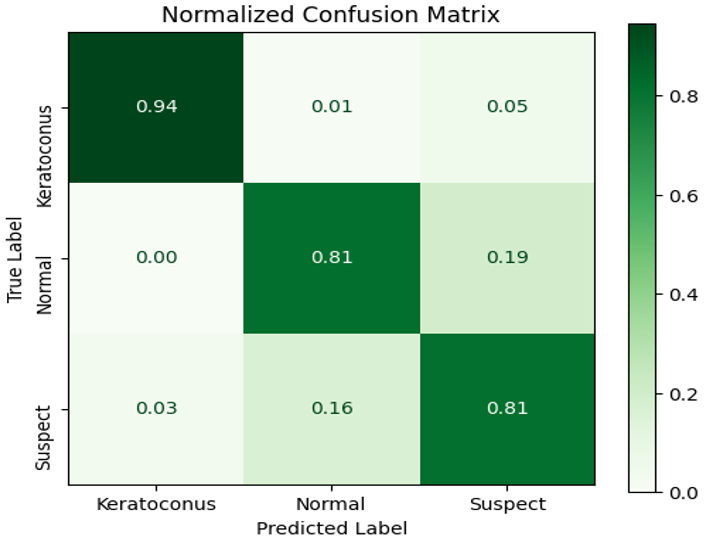
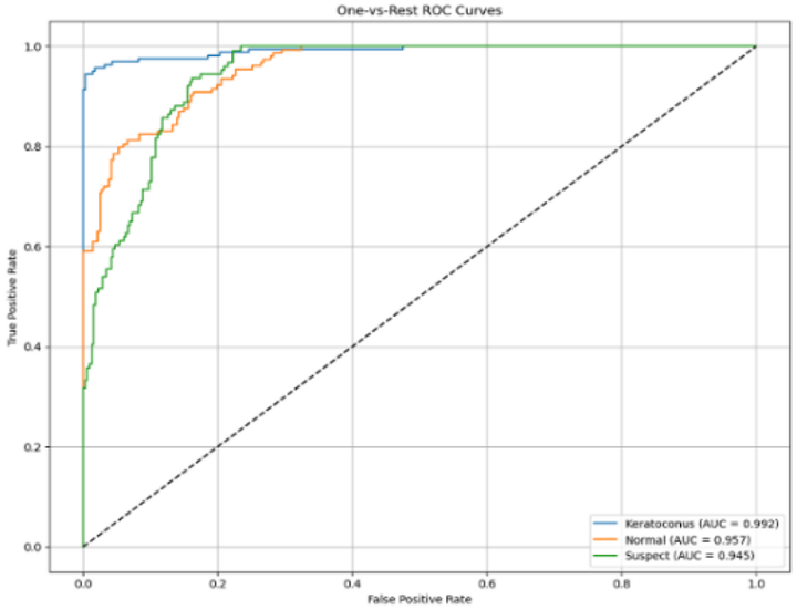
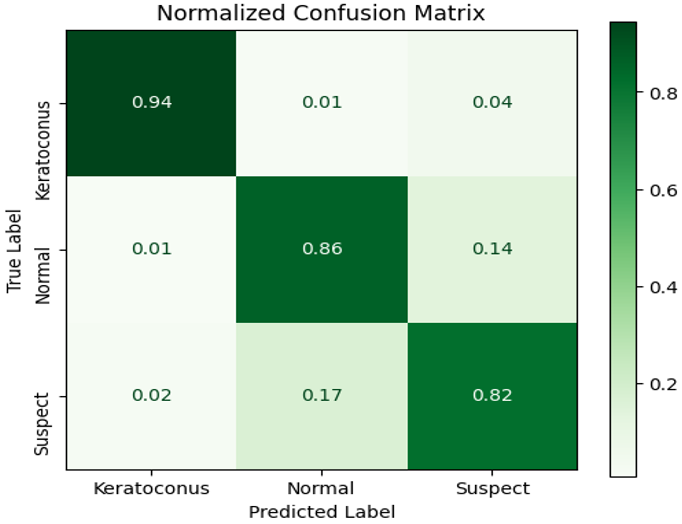
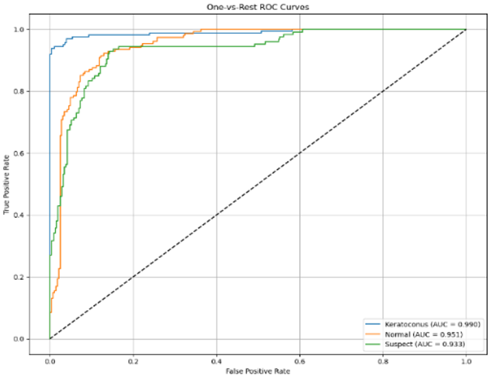
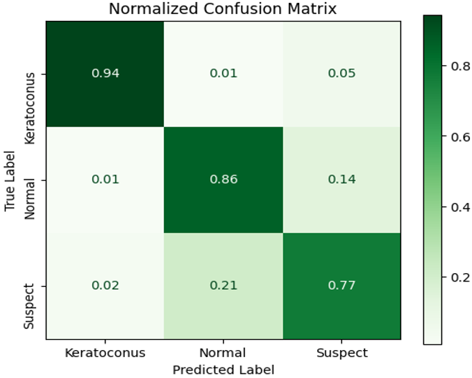
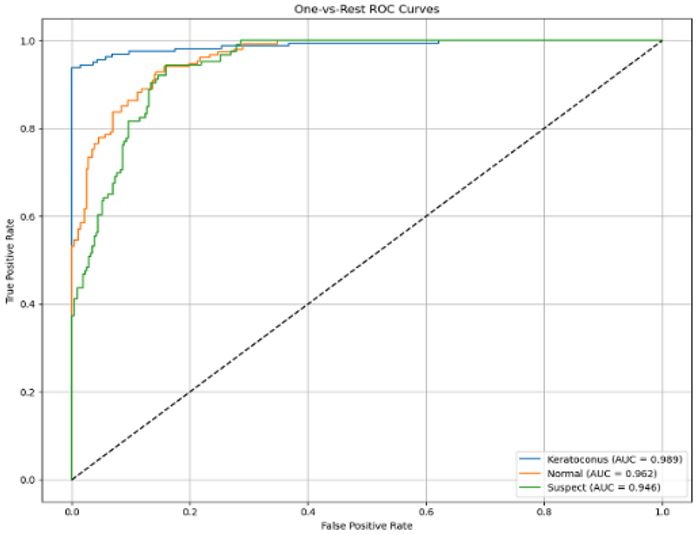
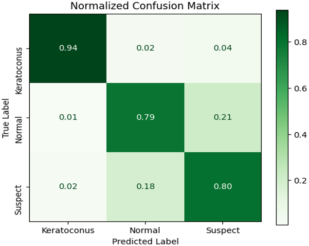
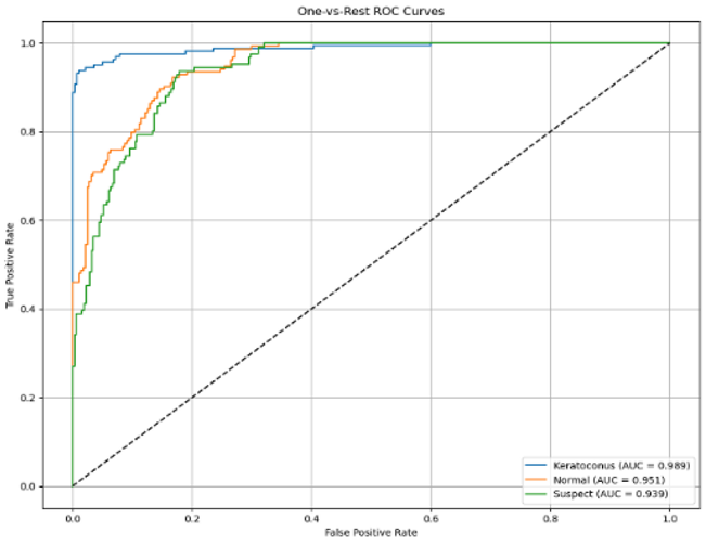
Figures 3–6 depict the normalized confusion matrices and ROC plots for all the 4 wavelets using the class weighting method.
Figure 3. Classification performance of the LightGBM classifier using bior1.5 wavelet: (a) Normalized confusion matrix plot (b) Receiver operating characteristic (ROC) curve
Figure 4. Classification performance of the LightGBM classifier using coif3 wavelet: (a) Normalized confusion matrix plot (b) Receiver operating characteristic (ROC) curve
Figure 5. Classification performance of the LightGBM classifier using db6 wavelet: (a) Normalized confusion matrix plot (b) Receiver operating characteristic (ROC) curve
Figure 6. Classification performance of the LightGBM classifier using rbio2.2 wavelet: (a) Normalized confusion matrix plot (b) Receiver operating characteristic (ROC) curve
Table 8 shows the effect of color space and decomposition level on classification performance with the class weighting method using a LightGBM classifier. The values report bootstrapped mean estimates (B = 1,000 test-set resamples).
Table 8. Ablation study of discrete wavelet transform (DWT) feature extraction components: Effect of color space and decomposition level on classification performance
|
Ablation |
Configuration |
Accuracy (%) |
Macro F1-Score |
Macro-AUC |
|
Color Space |
L*a*b* |
87.78 |
0.8727 |
0.9580 |
|
RGB |
85.50 |
0.8478 |
0.9537 |
|
|
Decomposition Level (coif3) |
Level 2 |
86.13 |
0.8585 |
0.9664 |
|
Level 3 |
86.86 |
0.8631 |
0.9619 |
|
|
Level 4 |
87.78 |
0.8727 |
0.9580 |
Table 9 shows the comparison between L1-LR and PCA as feature selection strategies for coif3 at decomposition level 4 with the class weighting method using a LightGBM classifier. The values report bootstrapped mean estimates (B = 1,000 test-set resamples).
Table 9. Ablation study of dimensionality reduction strategy: comparison of L1-LR against Principal Component Analysis (PCA)
|
Configuration |
Accuracy (%) |
Macro F1-Score |
Macro-AUC |
|
L1-LR |
87.78 |
0.8727 |
0.9580 |
|
PCA |
79.59 |
0.7844 |
0.9104 |
Table 10 shows the classification performance of the SVM, RF, XGBoost, and LightGBM classifiers with the class weighting method at decomposition level 4 with the coif3 wavelet. The values report bootstrap mean estimates (B = 1,000 test-set resamples).
Table 10. Ablation study of classifier choice
|
Configuration |
Accuracy % [95% CI] |
Macro F1-Score [95% CI] |
Macro-AUC [95% CI] |
|
LightGBM |
87.78 [84.58-90.48] |
0.8727 [0.8408-0.9013] |
0.9580 [0.9422-0.9726] |
|
SVM |
82.36 [78.68-85.71] |
0.8174 [0.7810-0.8518] |
0.9369 [0.9182-0.9546] |
|
Random Forest |
85.50 [82.54-88.66] |
0.8499 [0.8189-0.8842] |
0.9637 [0.9515-0.9748] |
|
XGBoost |
87.28 [84.13-90.25] |
0.8686 [0.8370-0.8994] |
0.9682 [0.9571-0.9780] |
Table 11 shows the classification performance of the LightGBM classifier using different wavelets for feature extraction at decomposition level 4. The table reports the accuracy percentages obtained on both the validation and test datasets with and without bootstrapping for each wavelet.
Table 11. Accuracy of Light Gradient Boosting Machine (LightGBM) classifier on validation and test sets with different wavelet functions using the class weighting method
|
Type of Wavelet |
Validation Set Accuracy (%) |
Test Set (Non-Bootstrapped) Accuracy (%) |
Test set (Bootstrapped Mean) Accuracy (%) |
|
bior1.5 |
80.27 |
85.94 |
85.98 |
|
coif3 |
80.95 |
87.76 |
87.78 |
|
db6 |
81.63 |
86.39 |
86.41 |
|
rbio2.2 |
81.41 |
84.58 |
84.59 |
Model evaluation metrics presented in Table 3 highlight the discriminative capacity of DWT-derived features. Among the wavelet families evaluated, coif3 achieved the highest accuracy (87.76%) and macro F1-score (0.8727), establishing it as the best-performing wavelet on primary classification metrics. However, db6 achieved higher macro-averaged area under the receiver operating characteristic curve (macro-AUC) (0.9658 vs 0.9580), suggesting stronger class discrimination performance across decision thresholds. Weighted average scores were calculated along with the macro average score, as the dataset is imbalanced.
Class-specific analysis in Table 4 further emphasizes the clinical relevance of these results. Keratoconus cases showed high recall (0.9441) across all wavelets. However, performance for suspect cases remained comparatively lower, with recall of 0.7698 for db6.
Statistical analysis was performed to validate the performance metrics obtained in Tables 3 and 4, and the results are presented in Table 5. The large F-statistic values and corresponding p-values below 0.001 across all five metrics suggest that differences in performance across the selected wavelets are not due to random variation. The post-hoc analysis using Tukey’s HSD test shows that adjusted p-values for almost all wavelet combinations are below the significance threshold of 0.05. The exception was the recall metric of bior1.5 vs db6, where no statistically significant differences were detected. Figures 3 to 6 depict the normalized confusion matrices with the corresponding ROC curves for keratoconus, normal, and suspect classes using the LightGBM classifier with a class weighting approach using bior1.5, coif3, db6, and rbio2.2, respectively.
Although SMOTE improved minority-class representation during training, its effect on suspect-class recall varied across wavelet families. The rbio2.2 wavelet demonstrated an improvement in suspect-class sensitivity, increasing from 0.8418 with class weighting to 0.8620 with SMOTE. The rest of the wavelets, bior1.5, coif3, and db6, exhibited a performance drop. These results suggest that the effectiveness of oversampling depends on the discriminative properties of the extracted wavelet features.
Table 6 shows the comparative performance of class weighting and SMOTE across five evaluation metrics for four wavelets. The paired t-test result indicates that the differences between the two class balancing strategies are statistically significant for all wavelets and all metrics with a p-value below 0.001. Positive mean difference values indicate that the SMOTE-based balancing technique achieved better average performance, whereas negative values suggest superior performance of the class weighting strategy. The bootstrapped mean values of almost all five metrics for the coif3 wavelet using the class weighting method are consistently higher, indicating a better discriminating capability in classifying keratoconus.
When compared against existing studies in Table 7, the proposed DWT-LightGBM framework demonstrates competitive performance. While, the study [23] reported a classification accuracy of 98% using a MobileNet V2-based deep CNN, it also relied extensively on image augmentation, resulting in a dataset exceeding 16,000 samples. This augmentation may have contributed to the reported performance. In contrast, our method achieved 87.76% accuracy using images without any augmentation, which supports the effectiveness of wavelet-based feature extraction approach. Validation and test accuracies in Table 11 show that the LightGBM model trained with coif3 achieved a mean accuracy of 87.78% and an associated 95% CI of [84.58%–90.48%] with bootstrapping, outperforming other wavelets. Moreover, all wavelets achieved test accuracies above 85%, indicating that features extracted by DWT remain highly informative for keratoconus detection.
Our prior study [34] used image pyramids and HOG for feature extraction to train the LightGBM classifier and achieved a mean accuracy of 85.64% with 95% confidence intervals ranging from 82.25% to 88.76%.
In study [34], the dataset was split at the image level, which could introduce data leakage. When the same study was re-evaluated using an eye-level split test accuracy remained similar, with 85.80% and 95%CI (82.54%–88.89%). The overlap between confidence intervals and the negligible difference in mean accuracy between the two approaches suggest that any leakage effect could not be detected due to limited sample size. The data split at eye level is methodologically preferred, but the dataset used is insufficient to show a statistically significant difference between the two approaches.
Unlike the HOG-based feature extraction strategy adopted in our earlier study [34], this study employed DWT to extract meaningful features. HOG extracts information from local gradient orientation patterns and typically requires construction of image pyramids to capture scale-dependent characteristics. Conversely, DWT provides a multi-resolution representation through recursive decomposition, simultaneously capturing approximation and detail coefficients at successive levels without requiring separate image pyramids.
HOG captures spatial gradient information but does not provide explicit frequency-band interpretation. The DWT-based approach decomposes each L*a*b* channel into distinct subbands across four decomposition levels, making it possible to evaluate the contribution of individual frequency bands in classification. This is not possible with HOG.
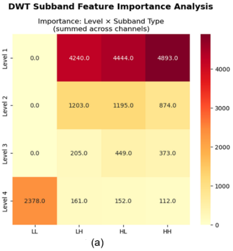
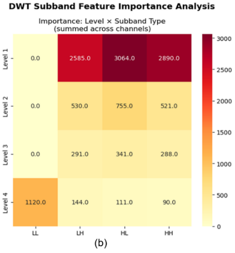
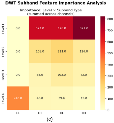
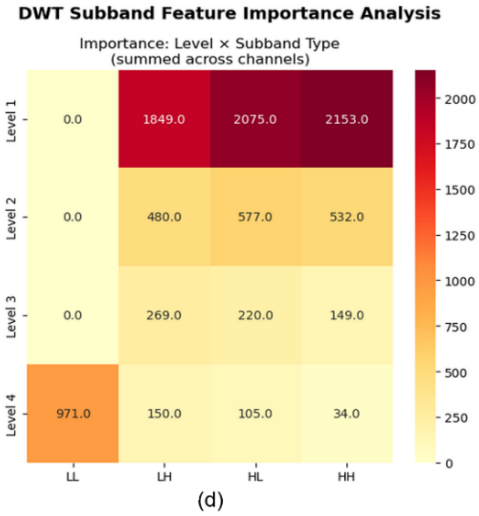
The subband importance results obtained from the four wavelet families in Figures 7(a)–(d) demonstrate a highly consistent pattern, indicating that the observed feature distributions are robust to variations in wavelet filter design. Across all wavelets, level 1 detail coefficients contributed more strongly to classification than coefficients from deeper decomposition levels, highlighting the importance of fine-scale information. The Coif3 heatmap in Figure 7(b) showed the strongest HL dominance, whereas the bior1.5 and db6 heatmaps in Figures 7(a) and (c) showed a weaker preference for HL.
In contrast, bior1.5 and db6 heatmaps from Figures 7(a) and (c) showed nearly equal contributions from HL and HH subbands, indicating that vertical edge and diagonal detail are equally informative. Although LL subbands at levels 2 and 3 contributed minimally, the level 4 LL approximation subband consistently showed significance, particularly for bior1.5, suggesting that coarse-scale shape information complements fine detail features.
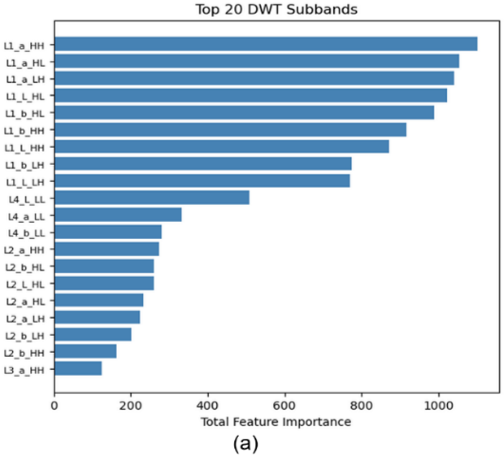
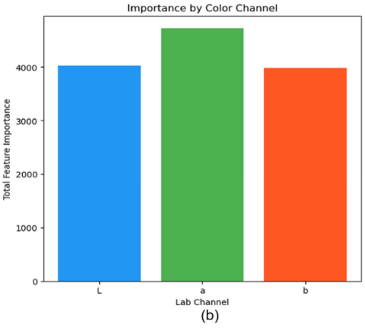
Figure 8(a) shows the top 20 subbands for the best-performing wavelet (coif3), with the highest-ranked features being predominantly of level 1. Figure 8(b) shows that the a* channel provided the largest share of feature importance. Unlike prior studies [34] that focused primarily on classification performance, this subband importance framework identifies the specific decomposition levels, subband orientations, and color channels driving the model decisions. This interpretability may facilitate future investigations into whether these patterns align with known clinical biomarkers.
Figure 7. Discrete wavelet transform (DWT) subband feature importance analysis of four wavelets: (a) bior1.5, (b) coif3, (c) db6, and (d) rbio2.2
Figure 8. Feature importance distribution of the best-performing wavelet (coif3) across: (a) discrete wavelet transform (DWT) subbands and (b) L*a*b* channels
The primary contribution of this work is threefold. First, applying the L*a*b* color space transformation before feature extraction improved classification accuracy by 2.28% over RGB pre-processing, as seen from the ablation study in Table 8. This demonstrates that perceptually uniform color representation improves the discrimination of corneal topography maps. Second, the subband-wise feature importance analysis (Figures 7 and 8) provides clinically interpretable insights into frequency domain components and color channels aiding in classification. Third, the supervised L1-regularized feature selection outperformed unsupervised PCA by 8.16% in accuracy, as shown in Table 9, highlighting the importance of class label-guided feature reduction for classification of keratoconus.
The ablation study in Table 8 shows that while decomposition level 4 achieved the highest accuracy and F1-score, level 2 produced the highest macro-AUC, indicating a trade-off between classification performance and probability calibration. The classifier ablation in Table 10 shows that while SVM performed worse, RF, XGBoost, and LightGBM exhibited comparable performance, with overlapping 95% CI levels. This suggests that improvement in performance could be attributed to feature representation rather than the classifier choice, although no formal statistical test was performed to compare the classifiers. In Table 9, PCA was applied to the scaled training features, which contained 197,184 dimensions. The number of retained components was set to n = 2078 according to the constraint min(n_selected, n_train-1). Here n_selected = 5112 represents L1-selected features, whereas n_train = 2079 denotes the number of training images. The retained 2078 PCA components explained 97.3% of the total variance. The dimensionality of the PCA baseline (2078) is lower than the L1-selected set (5112) due to this constraint.
Our proposed approach outperformed earlier works done in studies [20, 22], which achieved 81.5% and 77.43% accuracy, respectively, using EfficientNetB0 + SVM and VGG19. However, limitations persist. The suspect class yielded the lowest recall across all wavelets (0.7698–0.8175), with misclassified suspect cases assigned to the normal class. This normal-suspect confusion is clinically important because it concerns discrimination of borderline cases. The class weighting partially mitigates this by increasing the training penalty for the suspect class. However, detecting suspect cases remains a fundamental challenge. All experiments were conducted on a single dataset source from Al-Timemy et al. [20], and external validation on an independent test set was not performed. Furthermore, cross-validation was not employed; instead, a fixed stratified split with 1000-iteration bootstrap CIs was used to estimate performance stability. The bootstrap confidence intervals presented in Table 10 were estimated using a test set of 63 eyes (441 images). Although bootstrap offers a reliable measure of uncertainty in the reported performance, the confidence interval widths may be influenced by the limited test set size. Consequently, these findings should be regarded as preliminary estimates rather than conclusive measures of population-level performance.
While transformer models [24-26] and augmentation approaches [23] reported higher accuracies, the proposed DWT-LightGBM framework provides several practical advantages for clinical use. First, the entire pipeline, including feature extraction, feature selection, and classification, can be executed without GPU hardware, making it suitable for healthcare settings with limited computational resources. Second, the feature importance analysis across DWT subbands improves model interpretability by highlighting the significance of HL subbands and level 4 decomposition, which are associated with clinically relevant corneal characteristics. Finally, the reported performance was achieved without data augmentation or synthetic image generation, allowing the results to reflect the model’s performance on the original data distribution. These characteristics make the proposed framework a practical and interpretable alternative for clinical applications where computational efficiency and model transparency are important.
Further studies should validate the proposed framework using larger, multi-center, independent cohorts before clinical deployment. While wavelet-based features offer strong interpretability, future work could explore hybrid approaches combining CNN feature maps with handcrafted features. To improve the detection of borderline cases, curriculum learning strategies could be employed to focus on the suspect-normal decision boundary.
This study introduced a machine learning framework for keratoconus identification from Pentacam-derived corneal topography data. The framework combined L*a*b* color space, DWT-based feature extraction, feature standardization, and classification using a LightGBM model. Among the evaluated wavelets, coif3 achieved the highest classification accuracy and macro F1-score. The integration of L1-regularized feature selection and randomized hyperparameter optimization further enhanced model robustness of the proposed framework. Statistical analysis results indicate that the wavelet selection significantly affected the classification performance.
Overall, the findings confirm the importance of wavelet decomposition as a feature extraction method in keratoconus classification.
[1] Rabinowitz, Y.S. (1998). Keratoconus. Survey of Ophthalmology, 42(4): 297-319. https://doi.org/10.1016/s0039-6257(97)00119-7
[2] Krachmer, J.H., Feder, R.S., Belin, M.W. (1984). Keratoconus and related noninflammatory corneal thinning disorders. Survey of Ophthalmology, 28(4): 293-322. https://doi.org/10.1016/0039-6257(84)90094-8
[3] Galvis, V., Sherwin, T., Tello, A., Merayo, J., Barrera, R., Acera, A. (2015). Keratoconus: An inflammatory disorder? Eye, 29(7): 843-859. https://doi.org/10.1038/eye.2015.63
[4] Jones-Jordan, L.A., Walline, J.J., Sinnott, L.T., Kymes, S.M., Zadnik, K. (2013). Asymmetry in keratoconus and vision-related quality of life. Cornea, 32(3): 267-272. https://doi.org/10.1097/ico.0b013e31825697c4
[5] Ferdi, A.C., Nguyen, V., Gore, D.M., Allan, B.D., Rozema, J.J., Watson, S.L. (2019). Keratoconus natural progression. Ophthalmology, 126(7): 935-945. https://doi.org/10.1016/j.ophtha.2019.02.029
[6] de Sanctis, U., Loiacono, C., Richiardi, L., Turco, D., Mutani, B., Grignolo, F.M. (2008). Sensitivity and specificity of posterior corneal elevation measured by Pentacam in discriminating keratoconus/subclinical keratoconus. Ophthalmology, 115(9): 1534-1539. https://doi.org/10.1016/j.ophtha.2008.02.020
[7] Hallett, N., Yi, K., Dick, J., et al. (2020). Deep learning based unsupervised and semi-supervised classification for keratoconus. In 2020 International Joint Conference on Neural Networks (IJCNN), Glasgow, UK, pp. 1-7. https://doi.org/10.1109/ijcnn48605.2020.9206694
[8] Gore, D.M., Shortt, A.J., Allan, B.D. (2013). New clinical pathways for keratoconus. Eye, 27(3): 329-339. https://doi.org/10.1038/eye.2012.257
[9] Cao, K., Verspoor, K., Sahebjada, S., Baird, P.N. (2020). Evaluating the performance of various machine learning algorithms to detect subclinical keratoconus. Translational Vision Science & Technology, 9(2): 24. https://doi.org/10.1167/tvst.9.2.24
[10] Gomes, J.A.P., Tan, D., Rapuano, C.J., et al. (2015). Global consensus on keratoconus and ectatic diseases. Cornea, 34(4): 359-369. https://doi.org/10.1097/ico.0000000000000408
[11] Early Treatment Diabetic Retinopathy Study Research Group. (1991). Grading diabetic retinopathy from stereoscopic color fundus photographs—An extension of the modified Airlie House classification. Ophthalmology, 98(5): 786-806. https://doi.org/10.1016/s0161-6420(13)38012-9
[12] Korot, E., Guan, Z., Ferraz, D., et al. (2021). Code-free deep learning for multi-modality medical image classification. Nature Machine Intelligence, 3(4): 288-298. https://doi.org/10.1038/s42256-021-00305-2
[13] Maile, H., Li, J.P.O., Gore, D., et al. (2021). Machine learning algorithms to detect subclinical keratoconus: Systematic review. JMIR Medical Informatics, 9(12): e27363. https://doi.org/10.2196/27363
[14] Ali, A.H., Ghaeb, N.H., Musa, Z.M. (2017). Support vector machine for keratoconus detection by using topographic maps with the help of image processing techniques. IOSR Journal of Pharmacy and Biological Sciences, 12(6): 50-58.
[15] Yousefi, S., Yousefi, E., Takahashi, H., et al. (2018). Keratoconus severity identification using unsupervised machine learning. PLoS ONE, 13(11): e0205998. https://doi.org/10.1371/journal.pone.0205998
[16] Lavric, A., Popa, V., Takahashi, H., Yousefi, S. (2020). Detecting keratoconus from corneal imaging data using machine learning. IEEE Access, 8: 149113-149121. https://doi.org/10.1109/access.2020.3016060
[17] Al-Sharify, N.T., Yussof, S., Ghaeb, N.H., et al. (2024). Advances in corneal diagnostics using machine learning. Bioengineering, 11(12): 1198. https://doi.org/10.3390/bioengineering11121198
[18] Chaari, A., Fourati Kallel, I., Daoud, H., Omri, I., Kammoun, S., Frikha, M. (2024). Automated feature selection for early keratoconus screening optimization. Biomedical Physics & Engineering Express, 11(1): 015039. https://doi.org/10.1088/2057-1976/ad9c7e
[19] Kuo, B.I., Chang, W.Y., Liao, T.S., et al. (2020). Keratoconus screening based on deep learning approach of corneal topography. Translational Vision Science & Technology, 9(2): 53. https://doi.org/10.1167/tvst.9.2.53
[20] Al-Timemy, A.H., Mosa, Z.M., Alyasseri, Z., et al. (2021). A hybrid deep learning construct for detecting keratoconus from corneal maps. Translational Vision Science & Technology, 10(14): 16. https://doi.org/10.1167/tvst.10.14.16
[21] Kallel, I.F., Mahfoudhi, O., Kammoun, S. (2023). Deep learning models based on CNN architecture for early keratoconus detection using corneal topographic maps. Multimedia Tools and Applications, 83(16): 49173-49193. https://doi.org/10.1007/s11042-023-17551-8
[22] Gandhi, S.R., Satani, J., Jain, D. (2022). Classification of keratoconus using corneal topography pattern with transfer learning approach. In Smart Innovation, Systems and Technologies, pp. 165-178. https://doi.org/10.1007/978-981-19-3571-8_18
[23] Ahmed, N., Rahman, M.M., Ishrak, M.F., Joy, M.I.K., Sabuj, M.S.H., Rahman, M.S. (2024). Comparative performance analysis of transformer-based pre-trained models for detecting keratoconus disease. arXiv preprint arXiv:2408.09005. https://doi.org/10.48550/ARXIV.2408.09005
[24] Lu, Y., Li, B., Zhang, Y., Qi, Y., Shi, X. (2025). CMVFT: A multiscale attention-guided framework for enhanced keratoconus suspect classification in multiview corneal topography. American Journal of Ophthalmology, 280: 87-105. https://doi.org/10.1016/j.ajo.2025.08.008
[25] Abdelmotaal, H., Hazarbasanov, R.M., Salouti, R., et al. (2025). A hybrid transformers-based convolutional neural network model for keratoconus detection in Scheimpflug-based dynamic corneal deformation videos. Journal of Ophthalmic and Vision Research, 20: 1-17. https://doi.org/10.18502/jovr.v20.17716
[26] Sujitha, S.M.S., Subiramoniyan, S., Mahil, J., Jarin, T. (2025). Metaheuristic-optimized swin transformer with SHAP explainability for keratoconus classification from corneal topography maps. International Ophthalmology, 45(1): 396. https://doi.org/10.1007/s10792-025-03744-7
[27] Kandakji, L., Balal, S., Stupnicki, A., et al. (2026). Data-driven detection of subclinical keratoconus via semi-supervised clustering of multidimensional corneal biomarkers. Ophthalmology Science, 6(2): 100998. https://doi.org/10.1016/j.xops.2025.100998
[28] Jawad, E.M., Hazim, H.J.M., Daway, G. (2022). Retinal image enhancement by using adapted histogram equalization based on segmentation and lab color space. International Journal of Intelligent Engineering and Systems, 15(3): 614-622.
[29] Harikumar, R., Vinoth Kumar, B. (2015). Performance analysis of neural networks for classification of medical images with wavelets as a feature extractor. International Journal of Imaging Systems and Technology, 25(1): 33-40. https://doi.org/10.1002/ima.22118
[30] Ryali, S., Menon, V. (2009). Feature selection and classification of fMRI data using logistic regression with L1 norm regularization. NeuroImage, 47: S57. https://doi.org/10.1016/s1053-8119(09)70217-4
[31] Chawla, N.V., Bowyer, K.W., Hall, L.O., Kegelmeyer, W.P. (2002). SMOTE: Synthetic minority over-sampling technique. Journal of Artificial Intelligence Research, 16: 321-357. https://doi.org/10.1613/jair.953
[32] Ke, G., Meng, Q., Finley, T., et al. (2017). LightGBM: A highly efficient gradient boosting decision tree. In Proceedings of the 31st International Conference on Neural Information Processing Systems (NIPS'17), Long Beach, California, USA, pp. 3149-3157.
[33] Field, A. (2018). Discovering Statistics Using IBM SPSS Statistics. Sage, London, UK.
[34] Geddada, P.T., Pullagura, R.K. (2025). A pyramid-based feature fusion framework for keratoconus detection using LightGBM. Ingénierie des Systèmes d’Information, 30(8): 2095-2104. https://doi.org/10.18280/isi.300815