Tarek H. M. Abou-El-Enien | Yousria Abo-Elnaga | Ashraf Almahalawy | Kamilia Mohammad*
© 2026 The authors. This article is published by IIETA and is licensed under the CC BY 4.0 license (http://creativecommons.org/licenses/by/4.0/).
OPEN ACCESS
Sequential decision-making problems are frequently formulated under the assumption that feasible decision sets are precisely specified. In many practical settings, however, such sets may be incompletely characterized or subject to boundary ambiguity, making conventional dynamic programming (DP) formulations difficult to apply directly. In this paper, a rough dynamic programming (RDP) framework is developed for multi-stage optimization problems in which feasible decision sets are represented by their lower and upper approximations. Within this framework, the lower approximation is used to represent decisions that can be regarded as certainly feasible, whereas the upper approximation encompasses decisions that may be feasible under the available information. An RDP algorithm is formulated by embedding these rough-set representations within the recursive structure of DP, thereby allowing a deterministic objective function to be optimized while the imprecision of the feasible region is explicitly retained. The sequential dependence of decisions across stages is preserved through stage-wise state transitions and recursive value-function evaluation. Three representative rough dynamic programming problems (RDPPs) are formulated and solved to demonstrate the implementation of our proposed framework and to examine its behavior under different forms of imprecise feasibility. The resulting solutions illustrate how lower and upper feasible approximations can be incorporated into multi-stage optimization without requiring the uncertain feasible region to be reduced to a single precisely defined set. This framework provides a systematic basis for extending DP to sequential optimization problems in which feasibility information is incomplete, imprecise or boundary-ambiguous. Furthermore, it establishes a foundation for further investigation of solution properties, computational efficiency, and decision robustness in rough optimization.
rough set theory, rough dynamic programming, multi-stage optimization, imprecise feasible sets, sequential decision-making, rough optimization
Contemporary real-world problems are frequently characterized by a lack of precision [1]. Such imprecision may stem from insufficient information to distinguish between distinct elements, necessitating the consideration of information granules. It may also arise from a computational preference for using coarse-grained information to obtain efficient solutions, even when more detailed information is available. Optimization problems are representative of real-world scenarios in which inherent imprecision (roughness) may be encountered. To address such imprecision, rough set theory (RST), a mathematical framework introduced by Pawlak [2] in 1982, has demonstrated significant effectiveness and has been extensively applied in the field of optimization owing to its ability to characterize rough concepts, including sets, numbers, and functions.
The study of optimization problems in rough environments has a well-established historical foundation. In 2006, Youness [3] initiated this field by investigating optimal solutions over a rough decision set and introducing the term rough single-objective programming problem (RSOPP) to describe problems involving a precise objective function and an imprecise decision set. Subsequently, Osman et al. [4] extended this framework in 2009 by considering rough objective functions, leading to the classification of RSOPPs into three distinct classes according to the location of roughness. A methodology was also developed for solving first-class problems, which are characterized by a precise objective function and an imprecise feasible set. More recently, Wahed Khalifa et al. [5] advanced RSOPP research by employing the concept of boundary regions to develop and solve a novel type of RSOPP in which roughness is present in the definition of the objective function. Beyond single-objective problems, rough programming has also been extended to multi-objective programming problems (MOPPs) involving rough data. For example, Atteya [6] presented a weighted-sum method for rough multi-objective programming problems (RMOPPs) with rough decision sets. Moreover, RST has been combined with the Technique for Order Preference by Similarity to Ideal Solution (TOPSIS) to address various types of optimization and decision-making problems. For instance, TOPSIS was extended by El-Feky and Abou-El-Enien [7] to solve MOPPs with rough interval parameters, while Abou-El-Enien et al. [8] developed a rough-TOPSIS strategy to resolve conflicts among multi-objective functions defined over a rough decision set. In addition, El Sayed et al. [9] employed another rough-TOPSIS-based methodology to address multi-choice rough bi-level multi-objective nonlinear programming problems. Furthermore, the concept of rough intervals has been incorporated into various optimization problems to account for roughness in coefficient determination [10-19].
While the incorporation of RST into operations research (OR) has grown considerably, its application within dynamic programming (DP) frameworks remains relatively underexplored. In practical decision-making contexts, deterministic models are often impractical due to insufficient precise data or the substantial computational costs associated with conventional dynamic models. Existing studies have been limited to specific situations, such as investment problems in which earnings are represented by imprecise approximate intervals [20, 21]. Consequently, a significant gap remains in the treatment of imprecision within the decision space. To address this gap, a new approach to dynamic programming problems (DPPs) is developed that focuses on rough feasible regions rather than rough parameters. A comprehensive framework for multi-stage decision-making within a rough feasible set is thereby established, with consideration given to the previously underexplored issues of reachability and feasibility elasticity. This study further investigates the emerging field of rough dynamic programming (RDP), with the main contribution being the proposal and application of a novel RDP algorithm for solving rough dynamic programming problems (RDPPs) characterized by roughness occurring exclusively within the feasible set.
The proposed RDP algorithm represents a hybrid method that uniquely combines the DP approach with RST. This synergy is particularly advantageous for facilitating sequential decisions across different stages while optimizing an objective function defined over a rough feasible set. The proposed algorithm reformulates the RDPP into precise optimization problems by considering two scenarios: an optimistic case, in which optimization is performed over the upper approximation, and a pessimistic case, in which optimization is performed over the lower approximation while considering the worst-case values within the boundary region. The DP approach is then employed to solve each reformulated problem through sequential decision-making across the stages. This adaptive method enables robust treatment of solution feasibility while maintaining computational efficiency and preserving the sequential nature of the decision process. The utility of the proposed algorithm is demonstrated through its successful application to an integer linear rough resource allocation problem, an integer nonlinear rough inventory management problem, and a linear RDPP. In each case, the objective function is crisply defined, whereas the feasible solution set is characterized by its lower and upper approximations. These results demonstrate the adaptability of the proposed algorithm to different types of RDPPs.
The remainder of this paper is structured as follows: Section 2 introduces the RDPP model and some key related definitions. Section 3 presents a flowchart and pseudocode to illustrate the proposed RDP algorithm. Section 4 demonstrates the applicability of the proposed algorithm through the solution of three different RDPPs. Finally, Section 5 presents the conclusions and outlines possible directions for future research.
In this section, an RDPP model is introduced in which the feasible region is imprecise and the objective function is precisely defined over a subset of the fine universe. Essential definitions are also provided.
Formally, an approximation space $A=(U, E)$ comprises a finite, non-empty universe $U$ and an equivalence relation $E \subseteq$ $U \times U$. This relation $E$ partitions $U$ into pairwise disjoint subsets (equivalence classes), containing indistinguishable elements [2, 22]. This partition constitutes the quotient set $\mathrm{U} / \mathrm{E}=\left\{Y_1, Y_2, \ldots, Y_m\right\}$, where $Y_1, Y_2, \ldots, Y_m$ are the classes' names. Consequently, the universe is viewed simultaneously as a fine (ground) universe of elements and a coarse (quotient) universe of equivalence classes [23]. The transitions between these views are managed by the 'detail' operator $d: 2^{\mathrm{U} / \mathrm{E}} \rightarrow 2^U$ and the 'coarsen' operator $c: 2^U \rightarrow 2^{\mathrm{U} / \mathrm{E}}$ [24].
An RDPP with a rough decision set is modeled as follows:
RDPP:
$\begin{array}{ll}\max . & f(\mathbf{x})=\left(f_1\left(x_1\right), \ldots, f_N\left(x_N\right)\right) \\ \text { s.t. } & \mathbf{x}=\left(x_1, \ldots, x_N\right) \in M \\ & M_L \subset M \subset M^U \\ & M_L, M^U \subseteq U\end{array}$
where, $M \subset U \subseteq \mathrm{R}^N$ denotes the feasible region that is roughly defined by its lower approximation $M_L$ and upper approximation $M^U . \mathbf{x}$ is an $N$-dimensional decision variable vector, and $f: U \rightarrow R$ is a precise scalar objective function whose domain is a subset of the fine universe $U$.
In RDPP, the objective function's optimal value $f^*$ is defined by its lower limit $\underline{f^*}$ and upper limit $\overline{f^*}$:
$\underline{f^*}=\max \{\alpha, \beta\}$
$\overline{f^*}=\gamma$
where, solutions to the following optimization problems are assumed to exist.
$\begin{gathered}\alpha=\max _{\mathbf{x} \in M_L} f(\mathbf{x})=\left(f_1\left(x_1\right), \ldots, f_N\left(x_N\right)\right) \\ \beta=\max _{Y \in c\left(M_{B N}\right) \mathbf{x} \in d(Y)} f(\mathbf{x})=\left(f_1\left(x_1\right), \ldots, f_N\left(x_N\right)\right) \\ \gamma=\max _{\mathbf{x} \in M^U} f(\mathbf{x})=\left(f_1\left(x_1\right), \ldots, f_N\left(x_N\right)\right)\end{gathered}$
The three problems presented above are deterministic DPPs that exhibit separability and monotonicity properties [25]. Owing to these properties, the problems can be solved using the classical DP approach, pioneered by Richard Bellman [26], which decomposes the original problem into a series of simpler sub-problems and combines their solutions.
For RDPP, four optimal solution sets are identified, encompassing all possible levels of feasibility and optimality:
(1) The set of surely-feasible, optimistically-optimal solutions:
$F_s O_o=\left\{\mathbf{x} \in M_L \mid f(\mathbf{x})=\overline{f^*}\right\}$
(2) The set of probably-feasible, optimistically-optimal solutions:
$F_p O_o=\left\{\mathbf{x} \in M_{B N} \mid f(\mathbf{x})=\overline{f^*}\right\}$
(3) The set of surely-feasible, expectedly-optimal solutions:
$F_s O_e=\left\{\mathbf{x} \in M_L \mid f(\mathbf{x}) \geq \underline {f^*}\right\}$
(4) The set of probably-feasible, expectedly-optimal solutions:
$F_p O_e=\left\{\mathbf{x} \in M_{B N} \mid f(\mathbf{x}) \geq \underline{f^*}\right\}$
Should the optimal solution fall within the lower approximation of the feasible set, these optimal solution sets collapse to a single set, the set of surely-feasible optimal solutions, which is defined as follows:
$F_s O=\left\{\mathbf{x} \in M_L \mid f(\mathbf{x})=\gamma\right\}$
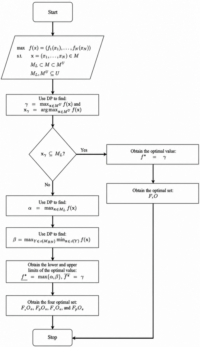
The proposed Algorithm 1 for addressing RDPPs employs a hybrid methodology that combines classical DP with RST. The core innovation lies in using the DP framework to find the values of $\alpha, \beta$ and $\gamma$.
Figure 1. Flowchart of the rough dynamic programming (RDP) algorithm
|
Algorithm 1. Rough dynamic programming (RDP) |
|
Input: $\begin{gathered}f(\mathbf{x})=\left(f_1\left(x_1\right), \ldots, f_N\left(x_N\right)\right), \text { opt } \in\{\max , \min \}, \\ F S=\left\{F S_1=M^U, F S_2=M_L,\right.\end{gathered}$ $\begin{gathered}\left.F S_3=d\left(Y_1\right), \ldots, F S_{2+c a r d}\left(c\left(M_{B N}\right)\right)=d\left(Y_{c \operatorname{ard}\left(c\left(M_{B N}\right)\right)}\right)\right\}, \\ t\left(s_n, x_n, F S_k\right), S_n\left(F S_k\right), s_1\end{gathered}$ Output: $\underline{f^*}, \overline{f^*}, F_s O_o, F_p O_o, F_s O_e, F_p O_e$ if opt $==\max$ then $\underline{f^*}=-\infty ;$ end if opt $==\min$ then $\overline{f^*}=\infty ;$ end for $k=1$ to $j+2$ do $current$$_{{opt}}=(k \leq 2)$? opt: $(($opt $==\max) ? \min:\max);$ for $n=N$ down to 2 do for each $s_n \in S_n\left(F S_k\right)$ do $X_n=(n==N) ?\left\{x_N \mid F S_k\right.$ constraints are satisfied$\}:$ $\left\{x_n \mid t\left(s_n, x_n, F S_k\right) \in S_{n+1}\left(F S_k\right)\right\} ;$ $V_n\left(s_n, F S_k\right)=$ $current$$_{{opt}}\left\{f_n\left(s_n, x_n\right)+((n==N) ? 0:\right.$ $\left.\left.V_{n+1}\left(t\left(s_n, x_n, F S_k\right), F S_k\right)\right)\right\} ;$ store $x_n^*\left(s_n, F S_k\right) ;$ end end $X_1=\left\{x_1 \mid t\left(s_1, x_1, F S_k\right) \in S_2\left(F S_k\right)\right\}$; $V^*\left(F S_k\right)={current}_{{opt}}\left\{f_1\left(s_1, x_1\right)+V_2\left(s_2, F S_k\right)\right\}$; store $x_1^*\left(s_1, F S_k\right) ; s_1^*=s_1$; for $n=1$ to $N-1$ do $x_n^*=x_n^*\left(s_n^*, F S_k\right) ; s_{n+1}^*=t\left(s_n^*, x_n^*, F S_k\right)$; end $x_N^*=x_N^*\left(s_N^*, F S_k\right) ; \pi^*\left(F S_k\right)=\left\{x_1^*, \ldots, x_N^*\right\}$; if $(k==1)$ and $\left(\pi^*\left(F S_1\right) \in F S_2\right)$ then return $f^*=V^*\left(F S_1\right), F_s O=\pi^*\left(F S_1\right)$; end if $k>1$ then if $\left((\right.$opt $==\max )$ and $\left.\left(V^*\left(F S_k\right)>\underline{f^*}\right)\right)$ then $\underline{f^*}=V^*\left(F S_k\right) ; \underline{\pi^*}=\pi^*\left(F S_k\right)$; end if $\left((o p t==\min )\right.$ and $\left.\left(V^*\left(F S_k\right)<\overline{f^*}\right)\right)$ then $\overline{f^*}=V^*\left(F S_k\right) ; \overline{\pi^*}=\pi^*\left(F S_k\right)$; end end end if $o p t==\max$ then $\overline{f^*}=V^*\left(F S_1\right) ; \overline{\pi^*}=\pi^*\left(F S_1\right) ; F_s O_o=\emptyset ; F_p O_o=\overline{\pi^*}$; $F_s O_e=\underline{\pi}^* \cap F S_2 ; F_p O_e=\underline{\pi^*} \cap\left(F S_1-F S_2\right)$; end if opt $==\min$ then $\underline{f^*}=V^*\left(F S_1\right) ; \underline{\pi^*}=\pi^*\left(F S_1\right) ; F_s O_o=\emptyset$; $F_p O_o=\underline{\pi}^* ; F_s O_e=\overline{\pi^*} \cap F S_2$; $F_p O_e=\overline{\pi^*} \cap\left(F S_1-F S_2\right)$; end |
In the RDP algorithm, $s_n$ represents the state of the system at stage $n, s_1$ is the initial state, and $t\left(s_n, x_n, F S_k\right)$ denotes the state transition function that determines the next state $s_{n+1}$ based on the current decision $x_n$ within the region $F S_k$.
From a system design perspective, our algorithm operates as a modular decision support system. The architecture consists of an analytical engine that processes rough constraint inputs, applies the recursive rough optimization, and outputs a set of optimal policies. This modularity can serve as a robust computational core for handling multi-stage imprecision.
Figure 1 provides a concise visual representation of the proposed RDP algorithm.
According to foundational theory of DP [26], any deterministic DP with a finite horizon and finite state space converges to an optimal policy. Therefore, because the proposed algorithm maps the rough feasible set onto a sequence of deterministic state-space environments, its convergence and optimality are naturally guaranteed.
This section demonstrates the procedural steps of the proposed RDP algorithm through its application to diverse mathematical structures. By focusing on these clear yet representative cases, a transparent verification is provided of how the boundary region of the decision set influences the optimal policy. These small-scale problems establish a baseline for future applications to large-scale systems, where heuristic methods may be required. The proposed algorithm is employed to solve an integer linear RDPP, an integer nonlinear RDPP, and a linear RDPP.
Example 1. (Rough integer resource allocation problem) A charitable organization has a $4,000 budget to support children with cancer. They aim to maximize the total bed capacity supported by distributing donations among three hospitals. The allocation is subject to two conditions: the contribution must be exclusively used for pediatric cancer treatment, and the full value of each selected stock must be paid. The hospital details are as follows:
(1) Hospital 1: children’s cancer, 33 beds, $2,000 per stock.
(2) Hospital 2: children’s cancer, 48 beds, $3,000 per stock.
(3) Hospital 3: all ages, 15 beds, $1,000 per stock; ineligible for child-exclusive donations.
Determine the stock allocation for each hospital that yields the maximum supported bed capacity.
Solution:
The objective is to ascertain the optimal allocation of shares to each hospital to maximize the total value of pediatric cancer support, constrained by a budget of $4,000. Let $x_n$ be the integer number of donation shares for hospital n, and let $U$ be the universe of all possible solutions defined by:
$\begin{aligned} U & =\left\{\mathbf{x}=\left(x_1, x_2, x_3\right) \in R^3 \mid 2 x_1+3 x_2+x_3\right. \left.\leq 4, x_1, x_2, x_3 \text { are non-negative integers }\right\}\end{aligned}$
The existence of $2^3=8$ distinct binary donation combinations for the three hospitals naturally generates an equivalence relation $E$ on $U$. This relation partitions the universe into a quotient set $U / E$ composed of eight equivalence classes, each corresponding to a unique donation strategy:
$U / E=\left\{Y_1, Y_2, Y_3, Y_4, Y_5, Y_6, Y_7, Y_8\right\}$
where,
$\begin{aligned} & d\left(Y_1\right)=\left\{\mathbf{x} \in U \mid x_1>0, x_2=0, x_3=0\right\} \\ & d\left(Y_2\right)=\left\{\mathbf{x} \in U \mid x_1=0, x_2>0, x_3=0\right\} \\ & d\left(Y_3\right)=\left\{\mathbf{x} \in U \mid x_1=0, x_2=0, x_3>0\right\} \\ & d\left(Y_4\right)=\left\{\mathbf{x} \in U \mid x_1>0, x_2>0, x_3=0\right\} \\ & d\left(Y_5\right)=\left\{\mathbf{x} \in U \mid x_1>0, x_2=0, x_3>0\right\} \\ & d\left(Y_6\right)=\left\{\mathbf{x} \in U \mid x_1=0, x_2>0, x_3>0\right\} \\ & d\left(Y_7\right)=\left\{\mathbf{x} \in U \mid x_1>0, x_2>0, x_3>0\right\} \\ & d\left(Y_8\right)=\left\{\mathbf{x} \in U \mid x_1=0, x_2=0, x_3=0\right\}\end{aligned}$
The mathematical formulation of this problem is:
$\begin{aligned} \max & f(\mathbf{x})=33 x_1+48 x_2+15 x_3 \\ \text { s.t. } & \mathbf{x} \in M \\ & M_L \subset M \subset M^U \\ & c\left(M_L\right)=\left\{Y_1, Y_2, Y_4, Y_8\right\} \\ & c\left(M^U\right)=U / E\end{aligned}$ (1)
The problem is formulated as a RDPP with a stage for each hospital $n=1,2,3$. At each stage, the decision variable $x_n$ represents the number of shares to contribute to the hospital $n$, while the state variable $s_n$ is the amount of money accumulated available for donation to hospitals $n, n+1, N$.
The stage return function, $r_n\left(x_n\right)$, is defined by $r_1\left(x_1\right)=$ $33 x_1, r_2\left(x_2\right)=48 x_2$, and $r_3\left(x_3\right)=15 x_3$.
Let $f_n\left(s_n\right)$ be the maximum return from contributions to hospitals $n, n+1, N$, the backward recursive relation can be constructed as follows:
$\begin{aligned} & f_3\left(s_3\right)=\max _{x_3}\left\{r_3\right\} \\ & f_n\left(s_n\right)=\max _{x_n}\left\{r_n+f_{n+1}\left(s_{n+1}\right)\right\}, n=1,2\end{aligned}$
To address the roughness of the feasible set, we apply the RDP algorithm shown in Figure 1. This includes a step where a crisp problem is solved to calculate the value of $\gamma$.
$\begin{aligned} \max & f(\mathbf{x})=33 x_1+48 x_2+15 x_3 \\ \text { s.t. } & 2 x_1+3 x_2+x_3 \leq 4 \\ & x_1, x_2, x_3 \text { are non-negative integers }\end{aligned}$ (2)
$s_{n+1}, n=1,2$ can be expressed as a function of $s_n$ using the following state transformation function: $s_2=s_1-2 x_1$, $s_3=s_2-3 x_2$.
Stage 3 computations:
$f_3\left(s_3\right)=\max _{x_3}\left\{15 x_3\right\}$
where, $x_3$ must be a non-negative integer that satisfies $x_3 \leq s_3$.
This yields:
$f_3\left(s_3\right)=\max _{x_3=0,1,2,3,4}\left\{15 x_3\right\}$
The computations for stage 3 are summarized in Table 1.
Table 1. Dynamic programming (DP) computation for stage 3
|
$15 x_3$ where $x_3 \leq \boldsymbol{s}_3$ |
Optimum Solution |
||||||
|
s3 |
x3 = 0 |
x3 = 1 |
x3 = 2 |
x3 = 3 |
x3 = 4 |
$f_3\left(s_3\right)$ |
$x_3^*$ |
|
0 |
0 |
- |
- |
- |
- |
0 |
0 |
|
1 |
0 |
15 |
- |
- |
- |
15 |
1 |
|
2 |
0 |
15 |
30 |
- |
- |
30 |
2 |
|
3 |
0 |
15 |
30 |
45 |
- |
45 |
3 |
|
4 |
0 |
15 |
30 |
45 |
60 |
60 |
4 |
Stage 2 computations:
$f_2\left(s_3\right)=\max _{x_2}\left\{48 x_2+f_3\left(s_3\right)\right\}$
where, $x_2$ must be a non-negative integer that satisfies $3 x_2 \leq s_2$.
This yields
$f_2\left(s_2\right)=\max _{x_2=0,1}\left\{48 x_2+f_3\left(s_2-3 x_2\right)\right\}$
The computations for stage 2 are summarized in Table 2.
Table 2. Dynamic programming (DP) computation for stage 2
|
$48 x_2+f_3\left(s_2-3 x_2\right)$ where $3 x_2 \leq s_2$ |
Optimum Solution |
|||
|
$s_2$ |
$x_2=0$ |
$x_2=1$ |
$f_2\left(s_2\right)$ |
$x_2^*$ |
|
0 |
0 |
- |
0 |
0 |
|
1 |
15 |
- |
15 |
0 |
|
2 |
30 |
- |
30 |
0 |
|
3 |
45 |
48 |
48 |
1 |
|
4 |
60 |
63 |
63 |
1 |
Stage 1 computations:
$f_1\left(s_1\right)=\max _{x_1}\left\{33 x_1+f_2\left(s_2\right)\right\}$
where, $x_1$ must be a non-negative integer that satisfies $2 x_1 \leq$ $s_1$.
This yields:
$f_1\left(s_1\right)=\max _{x_1=0,1,2}\left\{33 x_1+f_2\left(s_1-2 x_1\right)\right\}$
The computations for stage 1 are summarized in Table 3.
Table 3. Dynamic programming (DP) computation for stage 1
|
$33 x_1+f_2\left(s_1-2 x_1\right)$ where $2 x_1 \leq s_1$ |
Optimum Solution |
||||
|
$s_1$ |
$x_1=0$ |
$x_1=1$ |
$x_1=2$ |
$f_1\left(s_1\right)$ |
$x_1^*$ |
|
4 |
63 |
63 |
66 |
66 |
2 |
Beginning with the backward pass from stage 1 , the maximum return is determined to be $f_1(4)=66$, with the optimal decision being to donate 2 shares, $x_1^*=2$. This choice consumes the entire available budget, resulting in $s_2=s_1-$ $2 x_1^*=4-2 \times 2=0$. With no funds remaining, the optimal decisions for stages 2 and 3 are consequently $x_2^*=0$ and $x_3^*=$ 0. Thus, the optimal solution to problem (2) is the decision vector $\left(x_1^*, x_2^*, x_3^*\right)=(2,0,0)$, which yields an optimal value of $\gamma=f_1(4)=66$. This solution means donating 2 shares to Hospital 1 and no shares to Hospitals 2 and 3. This allocation fully complies with the condition that all funds must be used exclusively for children with cancer, making it a surely feasible outcome. The maximum value of 66 for problem (1) is therefore obtained by implementing this policy.
Example 2. (Rough integer non-linear inventory problem) Consider a two-month production-planning problem in which a factory must supply 60 electric heaters by the end of the first month and 150 by the end of the second month. The manufacturing cost of
electric heaters is defined by the quadratic function $\$\left(25 x+0.1 x^2\right)$. The cost of storing a unit until the next month is $4. A crucial condition, related tomaking the best use of the factory’s workforce and equipment, leads to a rough constraint on the first month’s production capacity. While any production exceeding 110 units is classified as "surely acceptable," the feasibility of producing 110 or fewer units is uncertain. The unique difficulty of the problem is that the precise threshold that separates acceptable and unacceptable production levels within this range is unknown. With no initial inventory, the factory seeks to minimize its total costs over the two months. The optimal production levels must be determined within this rough set of feasible capacities.
Solution:
The objective is to determine the optimal number of electric heaters to be produced in the first and second months to minimize overall manufacturing and warehouse expenses while satisfying demand and the operational constraints.
Let $x_n$ be the integer number of heaters produced in month $n$ (for $n=1,2$), and let $s_n$ be the integer inventory at the beginning of month $n$, with $s_1=0$. The problem's objective is to minimize the following crisp total cost function:
$\operatorname{cost}\left(x_1, x_2\right)=25 x_1+0.1 x_1^2+25 x_2+0.1 x_2^2+4 s_2$
The set of all possible production vectors defines the universe of the problem, U, such that:
$\begin{gathered}U=\left\{\mathbf{x}=\left(x_1, x_2\right) \in R^2 \mid 60 \leq x_1 \leq 210, x_1+x_2\right. \left.=210, x_1, x_2 \text { are integers}\right\}\end{gathered}$
The uncertainty in the first month's production capacity is formalized using RST. An equivalence relation $E$ partitions the universe of solutions $U$ into equivalence classes, forming the quotient set $U / E$:
$U / E=\left\{Y_1, Y_2\right\}$
where,
$\begin{gathered}d\left(Y_1\right)=\left\{\mathbf{x} \in U \mid 60 \leq x_1 \leq 110\right\} \\ d\left(Y_2\right)=\left\{\mathbf{x} \in U \mid x_1 \geq 111\right\}\end{gathered}$
This coarse-grained representation is used to define a rough feasible region, M, by its lower and upper approximations. These approximations are defined based on the production’s policy regarding resource usage levels.
$\begin{aligned} & c\left(M_L\right) \subset c(M) \subset c\left(M^U\right) \\ & c\left(M_L\right)=\left\{Y_2\right\} \\ & c\left(M^U\right)=U / E\end{aligned}$
This problem is considered a two-stage single-objective DPP (SODPP). Each month, $n=1,2$, represents a stage. At every stage, the decision variable is $x_n$, while the state variable is $s_n$. The stage cost function, $\operatorname{cost}_n\left(x_n, s_n\right)$, denotes the production and storage expenses for stage $n$:
$\begin{aligned} & \operatorname{cost}_1\left(x_1, s_1\right)=25 x_1+0.1 x_1^2 \\ & \operatorname{cost}_2\left(x_2, s_2\right)=25 x_2+0.1 x_2^2+4 s_2\end{aligned}$
Let $f_2\left(x_2, s_2\right)$ be the minimum cost incurred in the second month given $s_2$ and let $f_1\left(x_1, s_1\right)$ be the minimum cost incurred over both months given $s_1$. The backward recursive relation is then constructed as follows:
$\begin{aligned} & f_2\left(x_2, s_2\right)=\min _{x_2}\left\{\operatorname{cost}_2\left(x_2, s_2\right)\right\} \\ & f_1\left(x_1, s_1\right)=\min _{x_1}\left\{\operatorname{cost}_1\left(x_1, s_1\right)+f_2\left(x_2, s_2\right)\right\}\end{aligned}$
By substituting the second-stage decision variable $x_2^*=$ $150-s_2$ into the second-stage cost function, the recursive relation can be restated more concisely to directly reflect the inventory at the beginning of the second month, $s_2=x_1-$ $60+s_1=x_1-60:$
$f_1\left(x_1, s_1\right)=\min _{x_1}\left\{0.2 x_1^2-38 x_1+9420\right\}$
This problem can be solved by applying the RDP algorithm. At first, a crisp problem that minimizes the total cost over $M^U$ is solved to determine the value of $\gamma$.
$\begin{array}{ll}\min & \operatorname{cost}(\mathbf{x})=\left(25 x_1+0.1 x_1^2\right)+\left(25 x_2+0.1 x_2^2\right) \\ & +4\left(x_1-60\right) \\ \text { s.t. } & 60 \leq x_1 \leq 210 \\ & x_1+x_2=210 \\ & x_1, x_2 \text { are integers }\end{array}$
From the recursive relation:
$f_1\left(x_1, s_1\right)=\min _{60 \leq x_1 \leq 210}\left\{0.2 x_1^2-38 x_1+9420\right\}$
This leads to an optimal policy of $\left(x_1^*, x_2^*\right)=(95,115)$, where the inventory from the first month determines the second month's production $s_2=95-60=35$, so $x_2^*=$ $150-35=115$. The total cost incurred for this solution is $\gamma=\operatorname{cost}(95,115)=f_1(95,0)=\$ 7615$. Since this solution does not fall within the lower approximation of the rough feasible region $M_L$, it is necessary to determine the values of $\alpha$ and $\beta$.
To determine the value of $\alpha$, a crisp problem that minimizes the total cost with the constraint defined by $M_L$ is solved.
$\begin{aligned} \min & \operatorname{cost}(\mathbf{x})=\left(25 x_1+0.1 x_1^2\right)+\left(25 x_2+0.1 x_2^2\right) \\ & +4\left(x_1-60\right) \\ \text { s.t. } & 111 \leq x_1 \leq 210 \\ & x_1+x_2=210 \\ & x_1, x_2 \text { are integers }\end{aligned}$
From the recursive relation:
$f_1\left(x_1, s_1\right)=\min _{111 \leq x_1 \leq 210}\left\{0.2 x_1^2-38 x_1+9420\right\}$
The optimal solution is determined by $x_1^*=111$, which leads to the policy $\left(x_1^*, x_2^*\right)=(111,99)$. The total cost associated with this policy is $\alpha=\operatorname{cost}(111,99)=$ $f_1(111,0)=\$ 7666.2$.
Since there is only one equivalence class in the boundary region, the value of $\beta$ can be obtained by solving a crisp problem that maximizes the total cost with the constraint defined by $M_{B N}$.
$\begin{aligned} \max & \operatorname{cost}(\mathbf{x})=\left(25 x_1+0.1 x_1^2\right)+\left(25 x_2+0.1 x_2^2\right) \\ & +4\left(x_1-60\right) \\ \text { s.t. } & 60 \leq x_1 \leq 110 \\ & x_1+x_2=210 \\ & x_1, x_2 \text { are integers }\end{aligned}$
From the recursive relation (after replacing the min operator with the max operator):
$f_1\left(x_1, s_1\right)=\max _{60 \leq x_1 \leq 110}\left\{0.2 x_1^2-38 x_1+9420\right\}$
The optimal policy is found to be $\left(x_1^*, x_2^*\right)=(60,150)$, and the associated total cost is $\beta=\operatorname{cost}(60,150)=f_1(60,0)=$ $\$ 7860$.
The rough optimal value of the total cost is defined by the calculated values of $\alpha, \beta$, and $\gamma$.
$\underline{cost^*}=\gamma=7615$
$\overline{\cos t^*}=\min \{\alpha, \beta\}=\min \{7666.2,7860\}=7666.2$
Therefore, $\cos t^* \in[7615,7666.2]$.
The corresponding optimal solution sets are:
$\begin{aligned} F_s O_o= & \left\{\mathbf{x} \in M_L \mid \operatorname{cost}(\mathbf{x})=\underline{\cos t^*}\right\}=\varnothing \\ F_p O_o= & \left\{\mathbf{x} \in M_{B N} \mid \operatorname{cost}(\mathbf{x})=\overline{\cos t^*}\right\}=\{(95,115)\} \\ F_s O_e= & \left\{\mathbf{x} \in M_L \mid \operatorname{cost}(\mathbf{x}) \leq \overline{\cos t^*}\right\}=\{(111,99)\} \\ F_p O_e= & \left\{\mathbf{x} \in M_{B N} \mid \operatorname{cost}(\mathbf{x}) \leq \overline{\cos t^*}\right\} \\ & =\left\{\mathbf{x} \in M_{B N} \mid \operatorname{cost}(\mathbf{x}) \leq 7666.2\right\}\end{aligned}$
The subsequent example is formulated as a general linear numerical model demonstrating the adaptability of the proposed approach. This instance serves as a representative template that can be directly applied to a range of real-world applications across different industries. Our approach provides a comprehensive methodology for multi-stage linear optimization problems involving rough feasible sets.
Example 3. (General rough linear problem) Let $U=\{\mathbf{x}=$ $\left.\left(x_1, x_2\right) \in R^2 \mid-6 \leq x_1 \leq 6,-6 \leq x_2 \leq 6\right\}$ be the universe, and let $E$ be an equivalence relation on $U$ inducing a partition $U / E=\left\{Y_1, Y_2, Y_3, Y_4, Y_5\right\}$, where the equivalence classes are defined in the fine universe as follows:
$\begin{aligned} & d\left(Y_1\right)=\left\{\mathbf{x} \in U \mid-5 x_1+4 x_2 \leq 16, x_1 \leq 0, x_2 \geq 0\right\} \\ & d\left(Y_2\right)=\left\{\mathbf{x} \in U \mid-5 x_1+4 x_2 \leq 16, x_1+4 x_2 \geq-8\right. \\ & \left.x_1 \leq 0, x_2<0\right\} \\ & d\left(Y_3\right)=\left\{\mathbf{x} \in U \mid 0<x_1 \leq 2,0 \leq x_2 \leq 4\right\} \\ & d\left(Y_4\right)=\left\{\mathbf{x} \in U \mid 0<x_1 \leq 2,-2 \leq x_2<0\right\} \\ & d\left(Y_5\right)=\left\{\mathbf{x} \in U \mid \mathbf{x} \in\left\{U-U_{n=1}^4\left\{d\left(Y_n\right)\right\}\right\}\right\}\end{aligned}$
We seek to solve the following optimization problem:
$\begin{aligned} \max & f(\mathbf{x})=2 x_1-3 x_2 \\ \text { s.t. } & \mathbf{x} \in M \\ & M_L \subset M \subset M^U \\ & M_L=d\left(Y_1\right) \cup d\left(Y_2\right) \\ & M^U=d\left(Y_1\right) \cup d\left(Y_2\right) \cup d\left(Y_3\right) \cup d\left(Y_4\right)\end{aligned}$
Solution:
The first step in the RDP algorithm involves addressing the following crisp problem to determine the value of $\gamma$.
$\begin{array}{cl}\max & f(\mathbf{x})=2 x_1-3 x_2 \\ \text { s.t. } & -5 x_1+4 x_2 \leq 16 \\ & x_1+4 x_2 \geq-8 \\ & x_1 \leq 2 \\ & x_2 \leq 4 \\ & x_2 \geq-2\end{array}$ (3)
The aforementioned problem is considered a two-stage SODPP involving five state variables. At each stage $n=1,2$, the decision variable is $x_n$, and the state vector is denoted as:
$\mathbf{s}_n=\left(s_{1, n}, s_{2, n}, s_{3, n}, s_{4, n}, s_{5, n}\right)$
$\mathbf{s}_2$ can be expressed in terms of $\mathbf{s}_1$ through the following state transformation function:
$\mathbf{s}_2=\left(s_{1,1}+5 x_1, s_{2,1}-x_1, s_{3,1}-x_1, s_{4,1}, s_{5,1}\right)$
The backward recursive relation relating $f_1$ to $f_2$ is:
$f_1\left(\mathbf{s}_1\right)=\max _{x_1}\left\{2 x_1+f_2\left(\mathbf{s}_2\right)\right\}$
where, $f_2\left(\mathbf{s}_2\right)=\max _{x_2}\left\{-3 x_2\right\}$.
The second-stage sub-problem is to find the value of $f_2$.
$\begin{gathered}f_2\left(s_{1,2}, s_{2,2}, s_{3,2}, s_{4,2}, s_{5,2}\right) = \max _{\max \left\{\frac{s_{2,2}}{4}, s_{5,2}\right\} \leq x_2 \leq \min \left\{\frac{s_{1,2}}{4}, s_{4,2}\right\}} \begin{array}{c}\left\{-3 x_2\right\} f_2\left(s_{1,2}, s_{2,2}, s_{3,2}, s_{4,2}, s_{5,2}\right) =-3 \max \left\{\frac{s_{2,2}}{4}, s_{5,2}\right\}\end{array}\end{gathered}$
where, $x_2^*=\max \left\{\frac{s_{2,2}}{4}, s_{5,2}\right\}$.
The first-stage sub-problem is to find the value of $f_1$.
$\begin{gathered}f_1\left(s_{1,1}, s_{2,1}, s_{3,1}, s_{4,1}, s_{5,1}\right) \\ =\max _{\max \left\{\frac{-s_{1,1}}{5}, s_{2,1}\right\} \leq x_1 \leq s_{3,1}}\left\{\begin{array}{c}2 x_1 \\ +f_2\left(s_{1,1}+5 x_1, s_{2,1}-x_1, s_{3,1}-x_1, s_{4,1}, s_{5,1}\right)\end{array}\right\}\end{gathered}$
By substituting the value of $f_2$, we derive the following result:
$\begin{gathered}f_1\left(s_{1,1}, s_{2,1}, s_{3,1}, s_{4,1}, s_{5,1}\right) \\ =\max _{\max \left\{\frac{-s_{1,1}}{5}, s_{2,1}\right\} \leq x_1 \leq s_{3,1}}\left\{2 x_1-3 \max \left\{\frac{s_{2,1}-x_1}{4}, s_{5,1}\right\}\right\}\end{gathered}$
By substituting the state vector $\mathbf{s}_1$ derived from the righthand side of the constraints in problem (3), the following result is obtained:
$f_1(16,-8,2,4,-2)=\max _{\frac{-16}{5} \leq x_1 \leq 2}\left\{2 x_1-3 \max \left\{\frac{-8-x_1}{4},-2\right\}\right\}$
Accordingly, the optimal value of problem (3) is given by:
$\gamma=f_1(16,-8,2,4,-2)=10 \quad$ at $\quad x_1^*=2$
The corresponding optimal value for $x_2$ is:
$x_2^*=\max \left\{\frac{s_{2,1}-x_1^*}{4}, s_{5,1}\right\}=\max \left\{\frac{-8-2}{4},-2\right\}=-2$
Given that $(2,-2) \notin M_L$, it is necessary to determine the values of $\alpha$ and $\beta$.
Consider the following problem to obtain the value of $\alpha$:
$\begin{array}{cl}\max & f(\mathbf{x})=2 x_1-3 x_2 \\ s . t . & -5 x_1+4 x_2 \leq 16 \\ & x_1+4 x_2 \geq-8 \\ & x_1 \leq 0\end{array}$ (4)
The optimal value for the problem (4) is $\alpha=$ $f_1(16,-8,0)=6$, and the optimal policy is $\left(x_1^*, x_2^*\right)=$ (0, -2).
To determine the value of $\beta$, two distinct crisp problems are solved.
Consider the following problem to obtain the value of $\beta_1$:
$\begin{array}{cl}\min & f(\mathbf{x})=2 x_1-3 x_2 \\ \text { s.t. } & x_1>0 \\ & x_1 \leq 2 \\ & x_2 \geq 0 \\ & x_2 \leq 4\end{array}$ (5)
The optimal solution to problem (5) is determined by $x_1^*=$ $0^{+}$, which leads to the policy $\left(x_1^*, x_2^*\right)=\left(0^{+}, 4\right)$, where $\beta_1=$ $f_1(0,2,0,4)=-12^{+}$.
Consider the following problem to obtain the value of $\beta_2$:
$\begin{aligned} \min . & f(\mathbf{x})=2 x_1-3 x_2 \\ \text { s.t. } & x_1>0 \\ & x_1 \leq 2 \\ & x_2 \geq-2 \\ & x_2<0\end{aligned}$ (6)
The optimal solution to problem (6) is determined by $x_1^*=$ $0^{+}$, which leads to the policy $\left(x_1^*, x_2^*\right)=\left(0^{+}, 0^{-}\right)$, where $\beta_2=$ $f_1(0,2,-2,0)=5\left(0^{+}\right)$.
Consequently,
$\beta=\max \left\{\beta_1, \beta_2\right\}=\max \left\{-12,5\left(0^{+}\right)\right\}=5\left(0^{+}\right)$
This yields the following values for the lower and upper limits of $f^*$:
$\underline{f^*}=\max \{\alpha, \beta\}=\max \left\{6,5\left(0^{+}\right)\right\}=6$
$\overline{f^*}=\gamma=10$
Remark 1. For any $z \in R$, we define $z^{-}=z-\epsilon$ and $z^{+}=$ $z+\epsilon$ where $\epsilon$ is an insignificant small positive quantity chosen by the decision-maker (DM).
The corresponding optimal solution sets are:
$\begin{aligned} & F_s O_o=\left\{\mathbf{x} \in M_L \mid f(\mathbf{x})=\overline{f^*}\right\}=\varnothing \\ & F_p O_o=\left\{\mathbf{x} \in M_{B N} \mid f(\mathbf{x})=\overline{f^*}\right\}=\{(2,-2)\} \\ & F_s O_e=\left\{\mathbf{x} \in M_L \mid f(\mathbf{x}) \geq f^*\right\}=\{(0,-2)\} \\ & F_p O_e=\left\{\mathbf{x} \in M_{B N} \mid f(\mathbf{x}) \geq f^*\right\}=\left\{\mathbf{x} \in M_{B N} \mid f(\mathbf{x}) \geq 6\right\}\end{aligned}$
A significant finding is that the proposed algorithm produces a solution comparable to that obtained using the method proposed in reference [4]. This finding indicates that the contribution of the proposed algorithm does not lie in achieving a marginally better numerical result, but rather in providing a coherent and applicable solution that explicitly accounts for the imprecise nature of the feasible set. Specifically, the proposed approach enables DMs to make successive, stage-by-stage decisions in a rough environment, a capability that existing methods do not explicitly provide.
Despite the promising results, this study has several limitations. First, although the proposed RDP framework relies on deterministic DP for the transformed problems, it may still be subject to the ‘curse of dimensionality’. Consequently, its computational scalability and direct applicability to multi-stage problems with high-dimensional state spaces may be limited. Second, the current approach assumes that the model coefficients are predefined and fixed, and therefore does not account for real-time changes in the problem context.
This study was motivated by the need for effective optimization techniques to address the challenges associated with roughness and sequential decision-making. To address these challenges, an algorithm for RDPPs has been developed. The proposed algorithm was applied to three distinct problems, demonstrating its effectiveness across different problem settings, including two practical applications. The primary contribution of this work is the establishment of a foundation for RDP. This research provides a basis for further investigations into this emerging field.
(1) Future studies may extend this work to RDP problems with rough objective functions, as well as problems involving rough-interval coefficients.
(2) It would be fruitful to expand the current study to solve rough multi-objective DPPs.
(3) To enhance realism, a vital subsequent step is to explore stochastic RDP and perform stability and parametric analysis.
(4) The advancement of approximate RDP algorithms utilizing heuristic and meta-heuristic methods to reduce computational complexity in large-scale problems represents a significant avenue for future research.
[1] Yao, Y.Y. (2015). Granular computing: Basic issues and possible solution. Technical Report, Department of Computer Science, University of Regina, Canada. https://www2.cs.uregina.ca/~yyao/PAPERS/basic.pdf.
[2] Pawlak, Z. (1982). Rough sets. International Journal of Computer & Information Sciences, 11(5): 341-356. https://doi.org/10.1007/bf01001956
[3] Youness, E.A. (2006). Characterizing solutions of rough programming problems. European Journal of Operational Research, 168(3): 1019-1029. https://doi.org/10.1016/j.ejor.2004.05.019
[4] Osman, M.S., Lashein, E.F., Youness, E.A., Atteya, T.E.M. (2011). Mathematical programming in rough environment. Optimization, 60(5): 603-611. https://doi.org/10.1080/02331930903536393
[5] Wahed Khalifa, H.A.E., Pamucar, D., Kacem, A.H., Afifi, W.A. (2022). A novel approach for characterizing solutions of rough optimization problems based on boundary region. Computational Intelligence and Neuroscience, 2022: 1-12. https://doi.org/10.1155/2022/8662289
[6] Atteya, T.E.M. (2016). Rough multiple objective programming. European Journal of Operational Research, 248(1): 204-210. https://doi.org/10.1016/j.ejor.2015.06.079
[7] El-Feky, S.F., Abou-El-Enien, T.H.M. (2018). Compromise solutions for rough multiple objective decision making problems. Australian Journal of Basic and Applied Sciences, 113-119. https://doi.org/10.22587/ajbas.2018.12.7.18
[8] Abou-El-Enien, T., Abo-Elnaga, Y., Mohammad, K. (2025). Topsis for multiple objective programming with rough decision set. Yugoslav Journal of Operations Research, 35(1): 113-134. https://doi.org/10.2298/yjor230614003a
[9] El Sayed, M.A., Farahat, F.A., Elsisy, M.A., Alsabaan, M., Ibrahem, M.I., Elwahsh, H. (2025). Two TOPSIS-based approaches for multi-choice rough bi-level multi-objective nonlinear programming problems. Mathematics, 13(8): 1242. https://doi.org/10.3390/math13081242
[10] Lu, H.W., Huang, G.H., He, L. (2011). An inexact rough-interval fuzzy linear programming method for generating conjunctive water-allocation strategies to agricultural irrigation systems. Applied Mathematical Modelling, 35(9): 4330-4340. https://doi.org/10.1016/j.apm.2011.03.008
[11] Jana, D.K., Maity, K., Roy, T.K. (2013). Multi-item production inventory model with fuzzy rough coefficients via geometric programming approach. OPSEARCH, 50(4): 475-490. https://doi.org/10.1007/s12597-013-0122-9
[12] Hamzehee, A., Yaghoobi, M.A., Mashinchi, M. (2014). Linear programming with rough interval coefficients. Journal of Intelligent & Fuzzy Systems, 26(3): 1179-1189. https://doi.org/10.3233/ifs-130804
[13] Saad, O.M., Emam, O.E., Sleem, M.M. (2015). On the solution of a rough interval three-level quadratic programming problem. British Journal of Mathematics & Computer Science, 5(3): 349-366. https://doi.org/10.9734/bjmcs/2015/13430
[14] Omran, M., Emam, O.E., Mahmoud, A.S. (2016). On solving three level fractional programming problem with rough coefficient in constraints. Journal of Advances in Mathematics and Computer Science, 12(6): 1-13. https://doi.org/10.9734/bjmcs/2016/21932
[15] Mardanya, D., Maity, G., Roy, S.K., Yu, V.F. (2022). Solving the multi-modal transportation problem via the rough interval approach. RAIRO-Operations Research, 56(4): 3155-3185. https://doi.org/10.1051/ro/2022131
[16] Ammar, E., Al-Asfar, A. (2022). A study of uncertainty multi-objective nonlinear programming problems for rough intervals. Journal of Intelligent & Fuzzy Systems, 42(6): 4821-4835. https://doi.org/10.3233/jifs-202586
[17] Shivani, Rani, D., Ebrahimnejad, A. (2023). On solving fully rough multi-objective fractional transportation problem: Development and prospects. Computational and Applied Mathematics, 42(6): 266. https://doi.org/10.1007/s40314-023-02400-z
[18] Shivani, Rani, D., Ebrahimnejad, A., Gupta, G. (2024). Multi-objective non-linear programming problem with rough interval parameters: An application in municipal solid waste management. Complex & Intelligent Systems, 10(2): 2983-3002. https://doi.org/10.1007/s40747-023-01305-y
[19] Shivani, Rani, D., Rizk-Allah, R.M. (2024). A study of uncertain 4D transportation problems with rough interval parameters and additional real-life factors. Applied Soft Computing, 163: 111920. https://doi.org/10.1016/j.asoc.2024.111920
[20] Ammar, E.E., Khalifa, H.A. (2015). Solving investment problem with inexact rough interval data through dynamic programming approach. Journal of Advances in Mathematics and Computer Science, 8(3): 238-245. https://doi.org/10.9734/bjmcs/2015/15849
[21] Kumar, P., Abd, H., Khalifa, E.-W., Afifi, W.A., Kumar, P. (2022). Solving interval investment problem in vague environment using dynamic programming approach. Authorea, 8-17. https://doi.org/10.22541/au.166879191.12043710/v1
[22] Luo, J.F., Shi, C.J., Yao, Y.Y. (2025). A trilevel framework of rough sets and granular rough sets: Characterizing existing models and formulating new models. Information Sciences, 718: 122376. https://doi.org/10.1016/j.ins.2025.122376
[23] Yao, Y.Y., Yang, J.L. (2022). Granular rough sets and granular shadowed sets: Three-way approximations in Pawlak approximation spaces. International Journal of Approximate Reasoning, 142: 231-247. https://doi.org/10.1016/j.ijar.2021.11.012
[24] Yao, Y.Y., Liau, C.J., Zhong, N. (2003). Granular computing based on rough sets, quotient space theory, and belief functions. In Foundations of Intelligent Systems, pp. 152-159. https://doi.org/10.1007/978-3-540-39592-8_21
[25] Mine, H., Fukushima, M. (1979). Decomposition of multiple criteria mathematical programming problems by dynamic programming. International Journal of Systems Science, 10(5): 557-566. https://doi.org/10.1080/00207727908941602
[26] Bellman, R. (1966). Dynamic programming. Science, 153(3731): 34-37. https://doi.org/10.1126/science.153.3731.34