Intelligent Beamforming for 5G Communication Systems Using AI-Based Deep Learning

First and foremost, the main goal of massive multiple-input multiple-output (MIMO) and beamforming in 5G communication systems is to meet the requirements of high data rate and very high capacity. These two factors lead to enhancing the services of 5G systems [1].

MIMO is employed as a key in 5G by using a massive number of antennas at the base station. Massive MIMO enables the base station to serve many users simultaneously by applying the concepts of spatial multiplexing and beamforming. In addition to higher capacity and data rate, energy efficiency and spectral efficiency will be enhanced, and interference will be reduced. Therefore, the overall performance of the network will be improved by applying these techniques.

Subsequently, the main idea of beamforming is directing the transmitted energy (including the sent message) from the sender to the receiver instead of spreading it in all directions. On the other hand, when the receiver listens to the signals sent from the transmitter directly. This way of communication improves the strength of the signal, and the effect of interference and noise will be decreased; these conditions will lead to higher throughput. It is important to note that beamforming is more suitable to be applied in the base station than in the user equipment (UE) due to its complexity and requirements [1].

Based on the definition of 3GPP, massive MIMO is used when the system has more than eight transmitters. It is an extended MIMO in order to have a large number of transmitters. Its main concept is based on the ability to use beams to send signals in different ways. This is evidenced if the system has an antenna with two transceiver branches; the transmitter can send two streams simultaneously to single user (RX) and when the transmitter has four antenna branches its ability is improved and he can send four streams at the same time to a certain user furthermore sending dual of two streams to two users working on the principle of Multi User MIMO (MU-MIMO). Along those lines, if the system has 64 antenna branches, it is able to transmit data to multiple users simultaneously.

On the whole, the number of transceivers is an important point in designing MIMO antennas. When the system has a higher number of transceivers, it needs to generate more beams to cover the required capacity. On the other hand, this situation will increase the cost of implementing the system. Figure 1 shows an example with 192 elements arranged as 12 vertical and 8 horizontal antennas, while each antenna has two different polarizations. Antenna gain is defined by the number of antenna elements; increasing the number of antennas will increase the gain. Moreover, the frequency is responsible for determining the antenna spacing. At low frequencies, the antenna's physical size will be larger.

tu_pian_1.png

Figure 1. The relation between the number of transmitters and the number of antenna elements in a massive multiple-input multiple-output (MIMO) system

In fact, the antenna gain and size are controlled by the number of antenna elements. Furthermore, the antenna size depends on the frequency. For example, at high bands, the antenna becomes smaller.

Subsequently, the number of antenna elements is an important point at the transmitters/receivers, even if it can be lower or equal to the number of antenna elements to cover the required capacity with a suitable gain.

Likewise, the number of MIMO streams can be lower than or equal to the number of transmitters/receivers because these streams define the capability of peak data rate, which depends on the capability of baseband processing.

Finally, in the situation where antenna elements are larger (in number) than transmitters/receivers, these additional elements will be added as more rows. Typically, a MIMO system has 192 antenna elements and 64 transmitters, which can support up to 16 streams; in this case, each transmitter/ receiver has three rows [2].

Even more important is the mechanism of controlling beamforming. The UE establishes a radio link, then starts to use Synchronization Signal Blocks (SSBs), which are used in determining the initial configuration of the beam for the device. For 5G new radio networks below 6 GHz, it can be up to eight beams. Each beam has an SSB, and all these SSBs are sent in different directions but with the same strength. On the other hand, a UE will receive each signal block of synchronization with a different strength. After that, the UE will inform the network of the best signal identifier (SSB ID) when it wants to connect to the network. This is done through the use of the Random Access Channel request way, which will be linked to the particular SSB.

When there is a radio bearer, it is important to modify the configuration of the beam so the network can keep tracking the device while it is moving out of the coverage area of the initial beam. Also, the strength of the signal can be improved by making the beam narrow to a particular device during the transmission to this device. This is done by including Channel State Information Reference Signal (CSI-RS) while transmitting data and asking the device at the same time to report back the status of the received data.

Moving on, beamforming has two ways of steering the beam: Either configuring the UE with a Radio Resource Control reconfiguration (RRC-Reconfiguration) message; the role of this step is beam reporting on the MAC layer of the protocol stack. As a result, the network will be able to collect information and manage signal energy. Now, there is an indication that there is an entry from the standard precoding matrix codebook (this will be returned as feedback to the network on the MAC layer). This codebook can be referenced as the Precoding Matrix Indicator (PMI). Subsequently, the UE will analyze all the incoming signals and prepare the required network guidelines to modify the beam properly. There is another way of beam steering; this method is done through instructing the UE to radiate periodic Sounding Reference Signals (SRSs). On the other hand, the base station knows the look of SRS transmissions, so it will compare them with the received signals and will update the status of the beam according to these signals.

In fact, using these two ways includes RRC messaging to make the beam active and update its controls only. After completing the configuration, the beam will send feedback reports in the uplink and commands in the downlink direction. These two controls will be included in the MAC layer without depending on more RRC messaging. This way will make feedback production and processing as fast as possible.

In case the UE loses the beam, a beam failure recovery procedure should be initiated. It is done by indicating a new SSB ID during the procedure of random access.

Additionally, RRC measurement reports will include all the results of beam measurement, which will be used for inter-cell mobility. For example, if the strength of the beam signal of the neighbor cell is higher than the strength of the signal in the current cell, then the signal should be treated on the MAC layer and the mobility level of the cell should be handled in the RRC layer [3].

The main contributions of this work can be summarized as follows: The proposed model-driven convolutional neural network (CNN) framework is used for intelligent beam selection in 5G communication systems by integrating physical channel modeling with supervised deep learning. Furthermore, synthetic beam power measurements are generated from a physics-based channel model and are used for training instead of relying on extensive measurement-based datasets. Also, the proposed system is evaluated and compared with conventional exhaustive beam search. In the proposed framework, the trained CNN directly predicts the optimal beam during online operation, so the beam sweeping overhead is reduced. On the other hand, to cover the evaluation in terms of practical applicability, the framework is validated under multipath fading channels and multi-user scenarios. The obtained evaluation was comprehensive under varying conditions, and the system is assessed using various metrics such as beam prediction accuracy, confusion matrix analysis, Top-K accuracy, beamforming gain loss, and cumulative distribution function (CDF) analysis. This way of assessment demonstrates the framework's effectiveness for accurate and efficient beam prediction.

The paper includes a comprehensive literature review of deep learning architectures for the intelligent beamforming technique in Section 2. All the details of the proposed model and its equations are included in Section 3, while the definitions of the proposed system performance metrics are clarified in Section 4. The results and comparisons with related state-of-the-art are discussed in Section 5. Finally, all the conclusions from this work are assessed and clarified in Section 6.

This section includes the proposed model-driven CNN specifications and methodology for beam selection, which is unified because the learning framework is derived depending on physical channel and beamforming models.

3.1 Channel model and beamforming

The channel and beamforming model is first introduced. The system has a single-user downlink beamforming system, and the base station has a uniform linear array (ULA) of antennas (N_t) for transmission. Beam selection is performed using the following weights [23]:

$W=\left[w_l, w_2, w_3, \ldots, w_{N_b}\right]$, with $\mathrm{N}_b=\mathrm{N}_{\mathrm{t}}$          (1)

The assumed model has narrowband propagation with a dominant line of sight (LoS) component, while the channel vector is [24, 25]:

$h=\frac{1}{\sqrt{N_t}} a(\theta)$          (2)

where, $\theta$ is the angle of departure (AoD); the value was set to a random value between -60 and $60^{\circ}$ and this range is a practical and physical choice [23]. Subsequently, $a(\theta)$ is the ULA steering vector and can be defined as:

$a(\theta)=\left[1, e^{j \frac{2 \pi d}{\lambda} \sin (\theta)}, \ldots, e^{j \frac{2 \pi d}{\lambda}\left(N_t-1\right) \sin (\theta)}\right]^T$         (3)

Note that $\mathrm{d}=\lambda / 2 \mathrm{~d}$, while $\lambda$ is the carrier wavelength.

Furthermore, the system depends on the discrete Fourier transform (DFT) due to orthogonality, and it is suitable for beam sweeping as mentioned in a previous study [26]. The received beamforming power according to beam b is [26]:

$P_b=\left|w_b^H h\right|^2, b=1, \ldots, N_b$         (4)

Finally, for the beamforming model, the index of the optimal beam will be:

$b^*=\arg \arg _b^{\max } P_b$          (5)

This equation demonstrates that the index of the optimal beam corresponds to the beam with maximum received beamforming power among all candidate beams. Due to this, the ground-truth label for each training sample is the index of the beam with the highest received power. Sometimes, multiple beams exhibit identical received power, which is the maximum (rare case). In this situation, the function max in MATLAB will choose the first occurrence of the maximum value and it will have a unique class label for CNN training and testing.

On the other hand, it is important to present the details of model-driven data generation and feature construction so that the whole system will be clear and integrated. The mentioned physical channel and beamforming models are used to generate training data, and this is the point that makes the proposed framework different from purely data-driven approaches. The beamforming powers are computed for each channel realization and all beams in dB. So the beam power vector will be:

$P=\left[P_1, P_2, \ldots, P_{N_b}\right]$          (6)

In the designed beam selection framework, a CNN is employed. The difference from the existing related CNN works in the following important aspects:

1. Most of the existing works use full CSI or complex channel matrices as the input to the CNN. The proposed model uses beam power measurements obtained from the beamforming codebook as input feature representation. Each sample includes the received power values, which correspond to the candidate beam. The used way of representation reduces the requirements for full channel estimation and lowers the system overhead.

2. The other meaningful difference is training with variable SNR (-5 dB to 15 dB) using random values within this range. This approach enables the CNN to learn how to predict the beam under different noise conditions and leads to improved robustness of the proposed model.

3. The dataset generation considers a multipath channel, which converges to practical wireless environments and allows the CNN model to learn beam selection behavior under realistic channel conditions.

So the novelty of the proposed framework lies in these three points, which enable low complexity and robust beam prediction without requiring full CSI estimation.

3.2 Measurement and estimation model

In fact, we consider the beam power vector defined in Eq. (6) as the measured input to the proposed CNN. Each element of the vector P represents the beamformed received power of the beam in the DFT beamforming codebook. These values are obtained from applying each beamforming vector to the received channel and computing the corresponding received power. In the offline dataset generation stage, the beam power is generated directly from the physical channel for all values. All these values are considered to be ideal and without any impairments, in order to enable the proposed CNN to learn the actual relationship between the measured beam power distribution and the optimal beam index.

On the other hand, the proposed framework is designed to work as a practical wireless communication system in which the beam power measurements may be affected by receiver thermal noise, channel estimation errors, analog-to-digital converter quantization, and hardware calibration imperfections. So, in practical implementation, the measured power of the beam can be expressed as

$\widehat{P}_b=P_b+\varepsilon_b$          (7)

where, $P_b$ is the b-th element of the ideal beam power vector defined in Eq. (6), and $\varepsilon_b$ is the measurement error, which is modeled as an additive zero-mean Gaussian random variable in this practical work environment. The robustness of the proposed beam selection system is further evaluated and clarified later in the sensitivity analysis in Section 5.

3.3 Model-driven convolutional neural network-based beam selection

CNN is a way to learn the relation between the beam power vector and the optimal beam index. CNN is used to implement this task because it is able to exploit the correlations among adjacent beams, and these correlations arise from the structure of ULA [27, 28].

The training was offline and supervised to obtain the predicted beam index $\hat{b}$ and to approximate the function:

$f_\theta=P \rightarrow \hat{b}$           (8)

where, Θ represents network parameters. CNN selects the beam through inference, and this task enables fast selection with minimal computations. The design of the CNN architecture is designed to capture the spatial structure of beam power patterns. It is a one-dimensional structure and has two convolutional layers; the kernel sizes are small in order to extract the correlations of local beams, and then batch normalization and ReLU activation are included in order to improve the stability and nonlinearity of training. Furthermore, fully connected layers are included to perform a high level of beam classification. This lightweight CNN achieves high accuracy and low computational complexity. Figures 2 and 3 show the flowcharts of the offline training phase and online (real-time) beam selection phase.

tu_pian_2.png

Figure 2. Offline training phase

tu_pian_3.png

Figure 3. Online beam selection phase

The proposed framework supposes that the input to the CNN is available, which is the received beam power measurements corresponding to the predefined beam codebook. Also, the proposed model does not remove the initial beam measurement stage, which is required to obtain these observations; instead, its main objective is to reduce the complexity of computations and the latency of decision by replacing iterative beam search in conventional beam selection with a single forward inference in the trained CNN. As a result, the reported overhead reduction relates to the beam selection process and the decision-making process instead of the beam measurement procedure. Therefore, the investigation of beam prediction from beam measurements represents an important direction for future work.

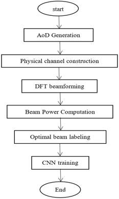
According to the reproducibility of the proposed framework, the following algorithm is included. It summarizes the implementation procedure completely during the online phase, i.e., model-driven dataset generation, CNN training, and beam prediction. Also, Table 1 includes all implementation details and hyperparameters to support any other assessment or comparison.

Table 1. The proposed convolutional neural network (CNN) architecture and training hyperparameters

5.1 Simulation setups

The framework of beam selection is evaluated by repeating it many times with a random AoD; for this reason, the system is evaluated through Monte Carlo simulations. As mentioned earlier, for a single-user downlink system, the base station is equipped with a ULA of 16 antennas. Also, the LoS channel model is considered, and the range of AoD within -60^o to 60^o.

The dataset has 10000 samples, which is partitioned into training, validation, and testing with ratios of 70%, 10%, and 20%, respectively. CNN is trained using the Adam optimizer; the learning rate is 0.001, the mini-batch size is 64, and the training epochs are 20. The training is offline and supervised, and the noise is considered free for all beams.

To cover all possible scenarios, the proposed framework was evaluated in two stages. Stage 1 used a noise‑free beam power dataset to establish the upper‑bound beam prediction performance under ideal conditions. Stage 2 used a more realistic dataset with multipath fading and an additive white Gaussian noise (AWGN) channel, with SNR values ranging from −5 to 15 dB to evaluate robustness in practical environments.

The noise was added during training and testing phases; each generated sample was corrupted by a randomly selected SNR value from the interval [-5,15] dB before beam power computation. This step is needed to cover realistic cases and to ensure that the CNN has the ability to predict beams with a high level of robustness under varying channel conditions (heterogeneous channel conditions), not only in ideal conditions.

Finally, for statistical robustness analysis, it is important to demonstrate that the experiment was completely repeated using ten independent random seeds. Each one of them generated different realizations of the channel, dataset portions, and CNN initialization and the mean and standard deviations were computed across independent runs.

5.2 Performance evaluation

5.2.1 Performance evaluation under ideal channel conditions

The evaluation of the proposed model-driven CNN is based on the evaluation of the performance metrics mentioned earlier. The first metric is accuracy, which is high, as shown in Figure 4.

tu_pian_4.png

Figure 4. Classification accuracy of the proposed model-driven convolutional neural network (CNN) under ideal channel conditions

tu_pian_5.png

Figure 5. Training loss of the proposed model-driven convolutional neural network (CNN) under ideal channel conditions

6.png

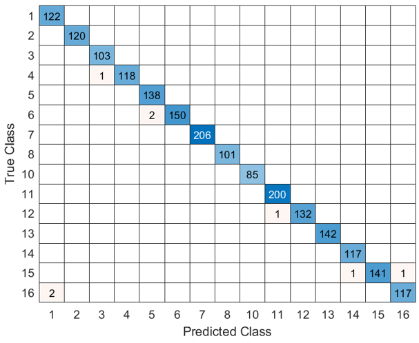
Figure 6. Confusion matrix for beam selection

It is clear that accuracy rapidly converges to 99.6% within early training epochs, and it is stable throughout the training process.

On the other hand, Figure 5 shows the training loss, which decreases sharply and approaches zero; this means the learning is effective, and the prediction is confident.

The system has no overfitting during the training process because of the agreement between training and validation accuracy. Also, the training time was short (1 minute and 6 seconds) for a single CPU, and this highlights the computational efficiency of the proposed system.

Figure 6 illustrates the confusion matrix of beam classification of the proposed system. It is clear that the major predictions are correct (along the main diagonal), which means the optimal beam index is identified properly for most channel realizations.

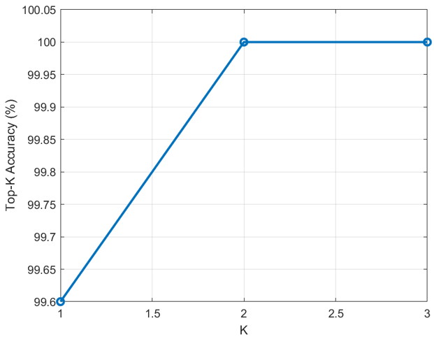
Figure 7 illustrates the Top-K beam selection accuracy. When K = 1, the accuracy is 99.6%, which means the predicted beam index matches the optimal beam, but when K is increased to 2 and 3, the accuracy reaches 100%, and this indicates the optimal beam is always included within the Top-K predicted candidates. In fact, this is a sign of the proposed system's robustness, which makes it suitable for practical beam management.

7.png

Figure 7. Top-K beam selection accuracy

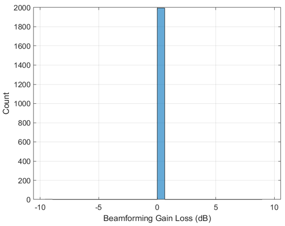
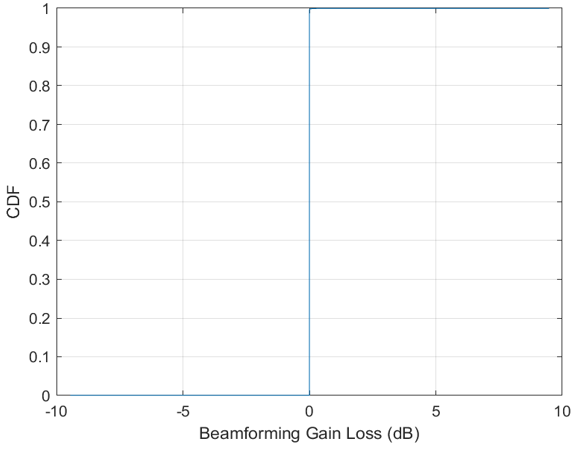
Figure 8 shows the histogram of beamforming gain loss between the optimal beam and the selected one (by the proposed system). The distribution around 0 dB indicates that the predicted beam is close to the optimal one. This highlights the effectiveness of the proposed model in maintaining beamforming gain because the misclassifications occur infrequently.

8.png

Figure 8. Histogram of beamforming gain loss

9.png

Figure 9. Cumulative distribution function (CDF) of beamforming gain loss

Table 2. Beamforming gain loss statistics for misclassified samples

Figure 9 shows the relation between the CDF and the beamforming loss. It is clear that beamforming gain loss remains near zero for most of the test samples, which indicates that the proposed CNN predicts the optimal (or near optimal) beam successfully in most cases. Subsequently, the beamforming gain loss was analyzed only for misclassified samples to assess the practical impact of prediction errors, as demonstrated in Table 2.

It is demonstrated in Table 2 that only 13 out of 2000 test samples were misclassified, i.e., for 0.65% of the samples, the average beamforming gain loss was 5.25 dB, while the maximum loss was 9.82 dB. Note that if multiple candidate beams exhibit nearly identical received power values, then zero gain loss occurs for a small number of misclassified samples. In fact, in these cases the predicted beam index differs from the reference label, but it has the same beamforming performance. For this reason, a conflict will appear between the beam prediction accuracy and the CDF due to the small proportion of sample misclassification and the existence of nearly equivalent beam candidates.

5.2.2 Performance evaluation under realistic channel conditions

To enrich simulation environments and have the best assessment of the system performance, realistic channel conditions are used:

1. Two paths are used with random angles and random gains to have a multipath channel.
2. Gaussian noise is added, which is scaled by SNR, so that the channel will be noisy.
3. Normalization is used to ensure the channel has unit power.

The proposed system is tested on a multipath fading channel with AWGN and the accuracy under these situations is shown in Figure 10.

It is clear that the proposed system performance is stable and the accuracy has fast convergence to 93.8% in validation over a realistic channel with varying SNR (-5 to 15 dB) along 2,180 iterations. For reproducibility, the number of training iterations is determined by dividing the training set size, which is 7000 (according to Table 1), by the mini-batch size, which is 64 (also taken from Table 1), so (7000/64) = 109 complete mini-patches, and with 20 epochs the total number of training iterations will be 109 × 20 = 2180 iterations. The remaining 24 samples (7000 – 109 × 64) do not form a complete mini-patch and are discarded for that epoch.

tu_pian_10.png

Figure 10. Classification accuracy of the proposed model-driven convolutional neural network (CNN) under realistic channel conditions

tu_pian_11.png

Figure 11. Training loss of the proposed model-driven convolutional neural network (CNN) under realistic channel conditions

On the other hand, the loss factor was also assessed under a multipath AWGN channel, and it was stable; the learning was also effective, and the loss converged to a near-zero value quickly, as shown in Figure 11. This value indicates that the degradation in physical layer performance is insignificant because the predicted beam is becoming very close to the target (optimum beam).

Subsequently, Table 3 demonstrates the principal performance indicators obtained under realistic channel conditions. The best achieved validation accuracy was 93.8% even when multipath propagation with AWGN existed, with random variations of SNR from -5 dB to 15 dB. Moreover, the decrease of training and validation loss was rapid and the levels converged to near-zero values, which proves that the learning behavior of the proposed framework was stable and the employed optimization technique was effective. Furthermore, the convergence and agreement between the training and validation curves, as shown in Figures 4 and 10, confirm that the proposed framework has no overfitting and generalizes well to unseen channel realizations. Overall, these results show that the proposed beam prediction framework is robust under practical channel conditions and environments and the system maintains reliable learning performance.

Table 3. Convolutional neural network (CNN) performance under realistic channel conditions

5.2.3 Sensitivity to measurement errors

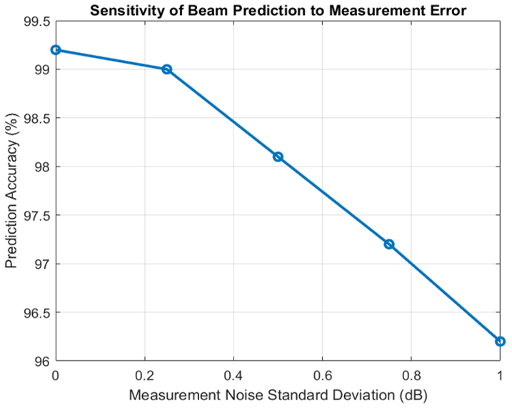
One of the most important metrics to assess the system is the robustness of the proposed framework under realistic environments, as mentioned earlier. For this reason, a sensitivity analysis was presented in this section and tested by introducing additive measurement errors into beam power measured values through the testing phase. As described in Section 3, the measurement error was modeled as an additive zero-mean Gaussian random variable in the dB domain, which represents the combined effects of all practical errors such as ADC quantization, thermal noise, and hardware calibration defects. The training of the CNN was done using the original dataset, while the measurement errors were introduced during the testing phase to highlight their impact on beam prediction performance.

Figure 12 shows that the standard deviation of measurement error was varied from 0 to 1 dB, while the corresponding beam prediction accuracies are summarized in Table 4.

12.png

Figure 12. The sensitivity of the proposed beam selection framework to measurement noise standard deviation

Table 4. Sensitivity of beam prediction accuracy to measurement errors

It can be demonstrated from Figure 12 and Table 4 that the proposed framework has a gradual degradation in prediction accuracy when the uncertainty of measurements increases, but the worst case has 95.75%, which means an absolute reduction of only 3.85 points. So the framework maintains prediction accuracy exceeding 95% and this indicates the framework demonstrated satisfactory robustness for practical beamforming systems.

5.2.4 Scalability potential

Scalability potential is beneficial to assess the performance of the proposed beamforming prediction for multi-user broadcasting on a multipath AWGN channel. The proposed framework is used to predict the beams of four users instead of one user as in previous simulations. The system is executed over 8,740 iterations to achieve stable convergence in the training process. Figure 13 illustrates how training accuracy increases rapidly and improves gradually to reach 93.65%, which means that the predicted beam is very close to the optimal beam, even when multiple users are present within the coverage area. The results indicate that the proposed model-driven CNN achieves scalability with accuracy comparable to that of the single-user scenario.

tu_pian_13.png

Figure 13. Classification accuracy of the proposed model-driven convolutional neural network (CNN) across four users

tu_pian_14.png

Figure 14. Training loss of the proposed model-driven convolutional neural network (CNN) across four users

Loss must be assessed to judge the performance fairly. The curve shown in Figure 14 supports the idea of scalability because of its sharp decrease to a near-zero value rapidly during the early iterations.

Furthermore, it is important to mention that the small gap between the accuracy curves in training and validation means that the model performs well on unseen data without overfitting. As a conclusion from these curves, they confirm that the proposed beam prediction framework achieves reliable learning performance and stable convergence for a multi-user (4 users) scenario.

Table 5. Convolutional neural network (CNN) performance in multi-user uniform linear array (ULA)-based beamforming scenario

Subsequently, Table 5 summarizes the principal quantitative results for the multi-user beam selection scenario. The proposed framework has the best validation accuracy of 93.65%, while the gain loss remains stable and near zero in the validation and testing phases. This level of performance (for single and multi-user scenarios) ensures the robustness, reliability, and scalability of the proposed model-driven CNN beam prediction framework.

5.2.5 Latency evaluation of beam selection

Latency means the required time to predict the optimal beam. It can be measured using the inference stage only because training is offline. The average inference time (total inference time/number of samples) is 20.3 µs per sample (on a PC with a Core i7 processor and 16 GB RAM). This value demonstrates that the proposed framework enables fast beam prediction suitable for real-time wireless communication systems.

In order to produce a practical perspective, the proposed CNN framework is compared with conventional beam sweeping. The optimal beam in the conventional approach is identified by evaluating all candidate beams sequentially, while the proposed framework predicts the optimal beam index through a single forward propagation when the beam power measurements are acquired. In this case, the latency of the reported beam selection is approximately 20 μs, which corresponds to the CNN inference stage measured in a MATLAB environment only without including beam measurement, signal acquisition, or hardware processing delays. As a result, this latency represents the computational cost of the beam prediction stage, not the end-to-end beam management latency and the result demonstrates that the proposed model provides an efficient mechanism with high beam prediction accuracy.

5.2.6 Reproducibility and statistical robustness analysis

In order to check the reproducibility and assess the statistical robustness of the proposed CNN-based beam prediction framework, the training and evaluation procedure was repeated over ten independent runs using different random seeds.

During data generation, SNR was independently sampled for each generated sample from a uniform distribution between -5 dB and 15 dB. The other hyperparameters, such as CNN architecture and evaluation setting, were kept unchanged throughout the experiments. This procedure ensures that the reported performance does not depend on a single experiment realization or random initialization.

Table 6. Statistical robustness of the proposed beam prediction framework over 10 independent runs

Table 6 demonstrates the statistical results obtained from the independent ten executions. The mean validation accuracy achieved by the proposed framework was 91.34 ± 0.93%, which indicates highly consistent convergence during training, even when the inherent randomness is introduced by channel generation, SNR sampling, and parameter initialization. Moreover, the average latency of beam selection was 0.0203 ± 0.0018 ms, which indicates that the system had a highly stable inference time, making it suitable for real-time beam prediction applications. Finally, the average training time was 47.57 ± 6.72 s, which means that the variation was moderate among different executions because of the stochastic optimization process employed by the Adam optimizer.

All these small deviations confirm the robustness and repeatability of the proposed CNN-based model and show that the model converges to similar performance for independent runs, so the reliability and reproducibility of the reported findings were improved.

5.2.7 The proposed framework comparison with baseline beam selection methods

In order to cover the performance of the proposed framework, a comparison with two baseline beam selection approaches is presented in this section using the same dataset and identical input features. The first baseline method depends on the conventional exhaustive beam sweeping, i.e., the selected beam has the maximum measured beam power. On the other hand, the second baseline is a lightweight multilayer perceptron (MLP) which is trained using the same beam power vector employed in the proposed framework. The main outcome from this comparison is the effectiveness of the proposed framework, which is evaluated under identical conditions.

Table 7 includes the quantitative comparison in terms of accuracy, Top-K accuracy, average beamforming gain loss, and inference time.

Table 7. Proposed framework comparison with baseline beam selection methods

The results show that the whole approach achieves high accuracy exceeding 99% and this indicates that the proposed model-driven CNN dataset enables highly reliable beam classification. On the other hand, the lightweight MLP achieves the higher Top-1 accuracy, but the difference to the proposed method is only 0.25%, which can be considered insignificant in practical applications. The important point is the inference time, which achieves 0.0203 ms for the proposed framework, i.e., the proposed CNN requires only this amount of time per prediction. In fact, the exhaustive beam sweeping method achieves perfect selection accuracy due to its direct evaluation of all candidate beams. As a result of sequential measurement of every beam in the codebook, the latency amount is proportional to the number of candidate beams and will be higher than that of learning-based inference. In contrast, the proposed framework needs a single forward propagation after acquiring the beam power measurements to predict the beam; this way reduces the computational complexity associated with the decision stage while near-optimal beam selection performance is maintained.

Putting it all together, the comparison demonstrates that the proposed model-driven CNN framework achieves a balance between prediction accuracy and computational complexity efficiency. After adding robustness analyses presented earlier, the results confirm the suitability of the proposed framework for practical beam selection applications due to its prediction reliability and low latency.

5.2.8 Computational complexity

The computational complexity of the proposed beam prediction system can be determined by the CNN that is used for 16-beam classification. Table 1 includes the proposed CNN architecture and training hyperparameters in calculations of the computational complexity.

Computational complexity is mainly determined by the convolution and fully connected layers during inference. The beam codebook size was 16, so convolution layer 1 has 1,536 multiplications, convolution layer 2 has 98,304 multiplications, fully connected layer 1 has 131,072 multiplications, and the output layer has 2,048 multiplications. Therefore, the total represents the computational complexity for one beam prediction, which is 232,960 (approximately 2.33 × 105).

The proposed model has a low level of computational complexity for the beam prediction scheme, which makes it efficiently implemented for real-time beam selection in mmWave communication systems.

5.2.9 Performance comparison vs. recent state-of-the-art

Table 8 illustrates the differences between the proposed model and recent related works. Even though the proposed work has a competitive level of performance compared to related approaches, there are two important advantages. Firstly, the system predicts the optimal beam using only beam power measurements, not camera images or location data. Moreover, the system operates under realistic channel conditions with random SNR, which ensures robustness in various communication environments. These advantages are observed through a comprehensive performance analysis of different metrics, including accuracy, loss, Top-K accuracy, beamforming gain loss, and CDF.

Table 8. Comparison of the proposed system with recent state-of-the-art methods