Muthusamy Saranya* | Rajasekaran Praveena
© 2026 The authors. This article is published by IIETA and is licensed under the CC BY 4.0 license (http://creativecommons.org/licenses/by/4.0/).
OPEN ACCESS
The classification of brain tumors needs reliable boundary localization and discrimination feature extraction to enhance diagnostic accuracy. In this paper, a hierarchical framework employing segmentation, feature extraction, feature selection, and classification of brain tumors using U-Net, Bendlet transform, Whale optimization, and a Fully Connected neural network. This approach initiates with the preprocessing of the input Magnetic Resonance Imaging (MRI) image, after which segmentation of tumors using a U-Net based architecture is performed to separate the region of interest. Furthermore, multidirectional features are extracted using the Bendlet transform from the segmented tumor area. The Bendlet transform is used to integrate the bending parameters to capture the curvature information. In addition, the Whale Optimization algorithm is utilized to select the most discriminative Bendlet features to minimize feature redundancy and irrelevant information from the high-dimensional feature space to improve discrimination capability. Moreover, the selected features are classified using a fully connected neural network into three types, which are meningioma, glioma, and pituitary tumor. The comparative analysis shows that to enhance the performance by increasing the directional value to an optimal level. The peak performance is achieved at eight directions, and level 3 decomposition gives 99.21%, 98.81%, and 99.39% of accuracy, sensitivity, and specificity.
Magnetic Resonance Imaging image, brain tumor, machine learning, Bendlet transform, Whale Optimization algorithm
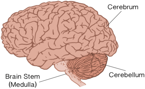
The Human Brain is the most essential and prime organ in our body. In the central nervous system, the intermediate organ is the human brain, along with the spinal cord. The main functions of the human brain and spinal cord in our body are to coordinate and control all our activities, such as thinking and intelligence, sensory processing, voluntary movements, and autonomic control, and this processed signal is sent to the remaining parts of the body. The human brain comprises three important regions: the cerebrum, cerebellum, and medulla oblongata. The functions of the cerebrum are thinking, memory, intelligence, and voluntary actions. Secondly, the function of the cerebellum is balance and coordination of muscles. At last, the functions of the Medulla oblongata control breathing and heartbeat. The detailed explanation of the three regions labelled is shown in Figure 1.
The Cerebrum is the largest part of the human brain and consists of two hemispheres. The names of the hemisphere is inner most and outermost. The innermost hemisphere is made up of white matter. Similarly, the outermost is commonly called the cerebral cortex, which is made up of grey matter. The white matter is for thinking and memory, and the grey matter is for signal transmission. Moreover, each hemisphere in the Cerebrum includes four lobes, namely the frontal, parietal, temporal, and occipital lobes. The frontal lobe is responsible for planning and decision making; likewise, the remaining three lobes are sensory information, emotional response, and visual processing. The connection between the spinal cord and the brainstem with help of cerebrum. The Cerebellum is the second largest region of the human brain, which is located below the cerebrum and at the back of the brainstem. The main function of the cerebellum is to coordinate voluntary movements. Next to the Medulla Oblongata, which is located at the lowest part of the brainstem. It is used to connect the brain to the spinal cord and is responsible for involuntary activities.
Figure 1. Anatomy of the human brain
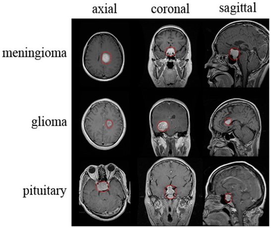
In the human brain, the abnormal growth of cells is called a brain tumor, which affects all brain activities because the human brain is responsible for all human activities. The brain tumors are classified into three types depending on the stages which are affected the brain. The primary brain tumors are benign and malignant, which originate in the brain. The examples of these tumors are Glioma, Meningioma, and pituitary. Similarly, the secondary tumors are malignant and spread over the brain to other organs. The examples of the tumors are lung, breast, kidney, and melanoma. The benign tumors are non-cancerous as well as slow growing and don’t spread over the brain, whereas malignant tumors are cancerous and fast growing over the brain. The diagnosis of a brain tumor is made by using Magnetic Resonance Imaging (MRI) and Computed Tomography (CT) imaging. In addition, detection and classification of brain tumors is done by deep learning-based algorithms, as shown in Figure 2.
Figure 2. Types of segmented tumors
The classification of brain tumors is a difficult task caused by irregular shape, heterogeneous texture, varying size, and uneven boundaries of tumor areas in MRI images. Along with, various tumor categories frequently give the same intensity distributions and overlapping structural characteristics, which affect accurate discrimination and classification. Compared with existing techniques such as Wavelet, Curvelet, Shearlet, and Contourlet transforms, which primarily focus on multiscale and directional feature representation, these techniques reveal several limitations in representing complex tumor regions. The Wavelet transform is limited in directional sensitivity for curved tumor boundaries, while the Curvelet transform is inefficient in capturing local bending and geometric variations. Moreover, the Shearlet transform is also affected by computational complexity and curvature adaptability; meanwhile, the contourlet transform is also unable to find accurate curvature details and uneven tumor regions. Overall, the drawback of existing transforms yields to minimize the capability of edge variations and curvature characteristics in brain tumors, computational complexity, and classification accuracy. To address these drawbacks, the proposed Bendlet transform integrates bending parameters that effectively capture the curvature-based multidirectional features and enhance the performance of tumor representation and classification.
Musallam et al. [1] have developed their framework and compared the existing network. The You Only Look Once Neural Architecture Search (YOLO NAS) model was used for the detection of various kinds of brain cancers with MRI images. While the datasets are taken from the REMBRANDT repository to enhance the classification process. The input images are preprocessed to eliminate the unwanted details before identifying the Region of Interests. HADF is employed to reduce noise. En-DeNet is utilized for encoding, whereas U-Net is used for Decoding [2].
Improved Deep Learning (DL) models are implemented to increase the efficiency and accuracy. While they utilized open source Kaggle datasets where it contains MRI images of glioma and meningioma. Several advanced structural modifications strengthen the process of capturing the important details and features [3].
This Models, like YOLOv5 and ResNet50 is combined, and YOLOv5 is employed to localize the tumor and for classification, whereas the combined framework of YOLOv5 and ResNet50 improves the feature extraction with histopathological images. The combined approach demonstrates effective identification of brain tumors. Several segmentation models were developed to enhance the detection of tumors [4]. They utilized various advanced components of YOLO, introducing the BTS-DS 2024 dataset with the models demonstrating accurate results [5].
The multimodal technique, which uses an enhanced deep learning framework, is applied to the BRATS dataset [6]. The first nine layers are trained for specialized preprocessing to achieve increased image quality, and the features were refined by applying well-optimized methodologies. It is classified into various tumor categories by utilizing a Support Vector Machine (SVM) model and Matrix-based merging of outcomes.
Improved ResNet50 Model integrates and replaces the original layers with four new layers to measure the effectiveness of accurate classification of cancer using DL techniques [7]. The CNN based techniques that address the problems in detail, loss, which is common in fully connected networks. The integration of multiscale feature extraction with U-Net captures all the details and the edges accurately [8]. While testing on The Cancer Genome Atlas Program (TCGA) dataset, it demonstrates higher performance.
The introduction of the Edge U-Net model, which uses MRI Boundary details, increases the accuracy of segmentation of tumors [9]. It uses Contrast Limited Adaptive Histogram Equalization (CLAHE) for preprocessing, and Edge-Guided Bridge (EGB) within the decoder that efficiently utilizes edge details, and the loss function is integrated. This method demonstrates a better dice score by utilizing the dataset having 3604 (T1-CE) data inputs [10].
The usage of the framework [11], which integrates deep learning and image processing, improves the segmentation process and brain tumor detection. It identifies the region of the tumor and enhances the boundaries to achieve increased accuracy. By utilizing the Br35H brain tumor dataset, this model demonstrates effective performance, 0.9391 for mAP@50, 0.4981 for mAP@50-95, 0.9681 for precision, and 0.9191 for recall. The development of the TL model [12]. which are incorporated with classifiers in order to categorize severity. This technique uses a U-Net based CNN to segment the affected areas. This method categorizes the glioma tumors into Low-Grade Glioma (LGG) and High-Grade Glioma (HGG).
CNN has been utilized in several studies to categorize brain tumors, according to Shafi et al. [13]. The work integrates ML and image classification techniques to differentiate multiple tumor classes. The Mask-RCNN and DL techniques are utilized for tumor localization and classification [14]. This approach marks an accuracy of 98.34% in the classification of tumor types. The model uses the DL approach of Alex Net's CNN via transfer learning, performed 97.62% of accuracy [15]. The hybrid technique that incorporates Genetic Algorithm and Social Spider Optimisation and uses ANFIS & SVM for the Classification distinguishes tumour and non-tumour regions by comparing [16]. This method demonstrates 99.72% of accuracy. The detection and classification can be done by several steps, and the CRAHB is applied to reduce the noise [17].
The method makes use of ML models for brain tumour classification with MRI images. Various models were evaluated [18]. Based on True Skill Statistics, the Decision Tree performance was the worst among those, whereas k-NN demonstrated good results. A work studied about diagnosis by using scanned MRI data, and they introduced the Boosted multi gradient SVM to classify the tumors [19]. Also, they introduced a Black Monkey Optimization-based SVM model. While this method demonstrated a remarkable performance of 99% accuracy. The work uses a CNN, a widely accepted DL technique, to detect and classify tumors with a dataset that contains T1-CE MRI input data [20]. Some work uses a deep CNN model with hyperparameters modified by a grid search optimizer to develop and demonstrate three different models for tumor classification [21, 22].
Multiscale Deep 3D CNN is developed to integrate both the global and local contextual information by utilizing a lower computational weight [23]. This will segment and classify glioma tumors into HGG and LGG and potentially make the tumor analysis more efficient and precise.
Initially, the MRI brain image as input data is taken and applied for the preprocessing steps to subtract the noise, then improve the contrast in order to increase the image quality. In addition, the preprocessed input image is given to a segmentation process, which is a U-Net based model that gives the exact tumor area from the preprocessed brain image. Moreover, distinguished features are effectively extracted by using the Bendlet transform from the segmented images, which yields curvature information of the tumor. In addition, the extracted features set may contain some redundant information. To avoid these issues, the Whale Optimization algorithm is used for optimization, which is to select more relevant features from the redundant information and also enhance the efficiency. At last, classification of tumors from the selected feature by using fully connected networks [24].
Figure 3 shows the proposed block diagram of tumor detection and classification system. This proposed framework ensures accurate tumor localization, optimized feature representation, and valid tumor classification.
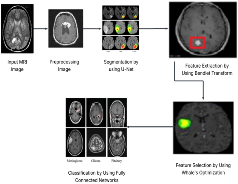
Figure 3. Block diagram of the proposed tumor detection and classification system
3.1 Bendlet transform
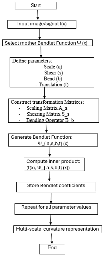
The Bendlet transform is a powerful tool that is used to represent images with curved contours, such as Brain images [3]. The transform starts by taking the input image or two-dimensional signal $f(x)$, where $x \in \mathrm{R} 2$, as the function to be analyzed. A mother bendlet function $\psi(x)$ is first selected, which serves as the generating function for constructing all bendlet atoms. This transform is built on four primary operators that define the 'bendlet' shape used to analyse the image, namely, Anisotropic scaling, Translation, Shearing $s \in$ R, and bending parameter $b \in \mathrm{R}$, which captures curvature information; and the translation parameter $t \in \mathrm{R} 2$, which localizes the analysis in space [24].
Using these parameters, the corresponding transformation operators are constructed. The anisotropic scaling matrix Aa applies parabolic dilation, the shearing matrix Ss adjusts orientation, and the bending operator Bb introduces a nonlinear curvature modification. These operators are combined with translation to generate the bendlet function.
$\Psi_{a, b, s, t}(X)=a^{-\frac{3}{4}} \Psi\left(A_a^{-1} S_s^{-1} B_b^{-1}(x-t)\right)$ (1)
where, the normalization factor a−3/4 ensures energy preservation in L2(R2).
The bendlet coefficients are then obtained by computing the inner product between the input signal and each bendlet function,
$\left(f, \Psi_{a, b, s, t}\right)$ (2)
which measures the presence of features at a specific scale, orientation, curvature, and spatial location. Eqs. (1) and (2) represent the process that is repeated for all combinations of the parameters a, s, b, and t. The resulting set of coefficients forms a multiscale, multi-orientation, and curvature-sensitive representation of the signal, providing detailed geometric information about edges and curved structures within the image, where ‘a’ represents anisotropic scaling parameter, captures features at multiple resolutions, s gives directional information, b gives curved structures, and t represents localizing the transform to specific regions of the image.
Figure 4 represents the flowchart of the Bendlet transform Algorithm. The bendlet transform is a second-order shearlet-based framework used to represent images with curved, discontinuous contours. While classical shearlets efficiently represent [25] anisotropic features such as edges with straight boundaries, bendlets incorporate curvature modeling to improve the sparse representation of curved singularities.
Figure 4. Flowchart of the Bendlet transform algorithm
The Shearlet transform is defined as:
$\varphi_{a, s, t}(x)=a^{-\frac{3}{4}} \varphi\left(A_a^{-1} S_s^{-1}(x-t)\right)$ (3)
Step 1:
The basic wavelet theory is defined by 1D:
$\varphi_{a, t}(x)=a^{-\frac{1}{2}} \varphi\left(\frac{x-t}{a}\right)$ (4)
Step 2:
The same idea applies in 2D:
$A_a=\left(\begin{array}{cc} a & 0 \\ 0 & a^{\frac{1}{2}} \end{array}\right)$ (5)
$x_1$ direction scales by a
$x_2$ direction scales by $a^{-\frac{1}{2}}$
The determinant is given by:
$\operatorname{det}\left(A_a\right)=a . a^{\frac{1}{2}}=a^{\frac{3}{2}}$
Step 3:
General rule for Matrix Scaling:
$\emptyset_A(x)=\emptyset\left(A^{-1} x\right)$ (6)
Then:
$\left\|\emptyset_A\right\|^2 L^2=\int_{R^2}\left|\emptyset\left(A^{-1} x\right)\right|^2$ (7)
Now perform a change of variable:
$y=A^{-1} x \rightarrow x=A y$ (8)
The Jacobian gives:
$d x=|\operatorname{det}(A)| d y$ (9)
Therefore,
$\left\|\emptyset_A\right\|^2 L^2=|\operatorname{det}(A)| \int|\emptyset(y)|^2 d y$ (10)
$\left\|\emptyset_A\right\|^2 L^2=|\operatorname{det}(A)|\|\emptyset\|^2 L^2$ (11)
To preserve energy, multiply by:
$|\operatorname{det}(A)|^{-1 / 2}$
Step 4:
Apply this to $A_a$:
$\operatorname{det}\left(A_a\right)=a^{\frac{3}{2}}$
The normalization factor must be:
$\left|\operatorname{det}\left(A_a\right)\right|^{-\frac{1}{2}}=\left(a^{\frac{3}{2}}\right)^{-\frac{1}{2}}=a^{-\frac{3}{4}}$ (12)
Step 5: Add shearing
The shearing matrix is given by:
$S_s=\left(\begin{array}{ll}1 & s \\0 & 1\end{array}\right)$ (13)
Now,
$\operatorname{det}\left(S_s\right)=1$
Shearing does not change area. Therefore, it does not affect normalization.
Step 6: Add translation
$x \rightarrow x-t$
Final derived equation is:
$\emptyset_{a, s, t}(x)=\left|\operatorname{det}\left(A_a\right)\right|^{-1 / 2} \emptyset\left(A_a{ }^{-1} S_s{ }^{-1}(x-t)\right)$ (14)
$\emptyset_{a, s, t}(x)=a^{-3 / 4} \emptyset\left(A_a{ }^{-1} S_s{ }^{-1}(x-t)\right)$ (15)
3.2 Whale Optimization algorithm
The Whale Optimization algorithm (Figure 5) is a technique to solve single- objective optimization problems. It will utilize three operators for the simulation: search for prey, encircling prey, and Bubble-net foraging behavior. The algorithm starts with the initialization of a random population of agents (whales), including the control parameters, such as the maximum number of iterations, the linearly decreasing coefficient a, and the spiral constant b. In each iteration, search agents update their positions relative to the effective solution among them and are identified as X, which is denoted as Prey.
A random number, PPP, is generated between 0 and 1 to decide the whale’s movement strategy. If the random number p < 0.5, the algorithm checks the magnitude of A.
If |A| < 1, the whale updates its position toward the best solution, by calculating a random value within an interval 0 to 1is called the exploitation phase. This mechanism is called the shrinking encircling mechanism. If |A| ≥ 1, the whale moves towards a randomly selected whale, enabling Exploration of the search space.
Figure 5. Flowchart of Whale Optimization algorithm
If the random number P ≥ 0.5, then it updates its position by calculating the distance between the whale and the prey, which is called the spiral equation, to simulate the bubble net attacking behaviour. After the fitness value is calculated, the best solution is calculated. As a result, the optimal solution is the one with the lowest fitness value of all search agents. This process repeats until the termination condition is met, at which point the algorithm outputs the best solution obtained.
3.3 Mathematical model for Whale Optimization algorithm
Key Steps and Equations
Always, whales choose the best solution and move around it. The equation is given by:
$\vec{D}=\left|\vec{C} . \vec{X}^*(t)-\vec{X}(t)\right|$ (16)
$\vec{X}(t+1)=\vec{X}^*(t)-\vec{A} . \vec{D}$ (17)
where,
$\vec{X}^*(t)$ is the best prey
$\vec{X}(t)$ is the current whale position
$\vec{A} . \vec{D}$ is the coefficient vectors
t is the current iteration
The calculation of $\vec{A}$ and $\vec{C}$:
$\vec{A}=2 \vec{a} . \vec{r}-\vec{a}$
$\vec{C}=2 . \vec{r}$
Steps used by Whales: shrinking encircling mechanism and spiral updating position.
Shrinking Encircling Mechanism
It is similar to the encircling mechanism, but the condition for moving closer to the prey is:
$\vec{A}<1$
Spiral updating position
The whales move around the prey, which looks like a helix-shaped path:
$\vec{X}(t+1)=\overrightarrow{D^{\prime}} . e^{b l} . \cos (2 \pi l)+\vec{X}^*(t)$ (18)
where,
$\overrightarrow{D^{\prime}}=\left|\vec{X}^*(t)-\vec{X}(t)\right|$ (19)
b is a constant defining a spiral shape
l is a random number
The total probability p is:
$\vec{X}(t+1)=\left\{\begin{array}{c}\vec{X}^*(t)-\vec{A} . \vec{D}, \quad P<0.5 \\\vec{D}^{\prime} . e^{b l} . \cos (2 \pi l)+\vec{X}^*(t), \quad P \geq 0.5\end{array}\right.$
When $|\vec{A}|>1$, the whales move away from the value:
$\vec{D}=\left|\vec{C} . \vec{X}_{{rand }}-\vec{X}(t)\right|$ (20)
$\vec{X}(t+1)=\vec{X}_{ {rand }}-\vec{A} . \vec{D}$ (21)
$\vec{X}_{ {rand}}$ is a random whale position.
Table 1 represents the Hypertuning parameters of the Whale optimization algorithm with Population Size, Maximum Iterations, Control Parameter, Coefficient Vector, Spiral Constant, and Random Number.
In Table 1, the values of hypertuning parameters of the whale optimization algorithm are based on convergence stability, feature selection efficiency, and computational complexity by using the trial and error method.
Table 1. Hypertuning parameters
|
S.No. |
Hypertuning Parameter |
Symbol |
Typical Range |
|
1 |
Population Size |
N |
50 |
|
2 |
Maximum Iterations |
T |
500 |
|
3 |
Control Parameter |
a |
2 to 0 |
|
4 |
Coefficient Vector |
A |
[-a,a] |
|
5 |
Coefficient Vector |
C |
[0,2] |
|
6 |
Spiral Constant |
b |
1 |
|
7 |
Random Number |
p |
0,1 |
3.4 Customized Convolutional Neural Network
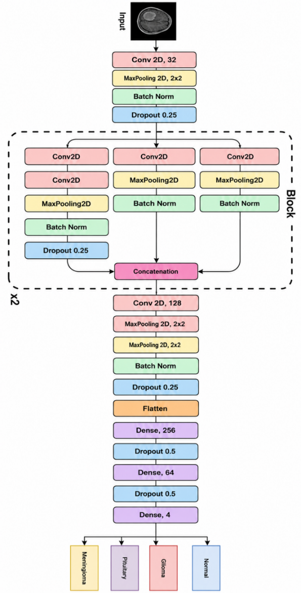
The Convolutional Neural Network (CNN) designed for brain tumors with MRI images is shown in Figure 6. It takes an input of MRI images via a Conv2D layer with 32 filters for extracting features like edges and textures. Maxpooling is applied to reduce spatial dimensions, Batch Normalization can stabilize and speed up the training process, and it drops out (0.25) in order to prevent overfitting.
Figure 6. Architecture of a fully connected neural network
This architecture uses convolutional blocks for two times repeatedly. These blocks can have Conv2D layers at different paths, Maxpooling, Batch Normalization, and the outputs combined by using a concatenation layer. The multi path structure enables the model to capture features from different scales, like Inceptional style design. After concatenation, a deeper feature extraction can be done using 5 × 5 and 3 × 3 Conv2D layers and 128 filters, Maxpooling, Batch Normalisation, and Dropout. The results are then flattened to a one-dimensional vector and passed into a fully connected layer, where it can include 256 neuron layers and 0.5 Dropout for regularisation. At last, we can get images with 4 categories: Normal, Glioma, Pituitary or Meningioma, which are classified by the output layer using a SoftMax activation function. Overall, this model integrates convolutional feature extraction, Multiscale learning, and a regularization technique in order to ensure precise multiclass brain tumor classification.
In this work, the brain tumor is diagnosed from MRI images of the brain under four types, namely normal, Glioma, Pituitary, and Meningioma. The dataset can be used for normal class 405 images, for Glioma, Pituitary, and Meningioma classes 300, 300, and 300, respectively. In that, the dataset was divided into training and testing in the ratio of 80:20, where 80% of the MRI images were used for training, and rest of the 20% were used for testing.
Table 2. Performance evaluation of the Bendlet transform
|
Dir |
Lev |
Performance Measures |
||
|
Accuracy |
Sensitivity |
Specificity |
||
|
2D |
1 |
82.99 |
74.48 |
87.22 |
|
2 |
86.43 |
79.65 |
89.80 |
|
|
3 |
89.21 |
83.81 |
91.89 |
|
|
4 |
85.88 |
78.81 |
89.39 |
|
|
4D |
1 |
89.99 |
84.98 |
92.47 |
|
2 |
93.21 |
89.91 |
94.89 |
|
|
3 |
95.99 |
93.98 |
96.97 |
|
|
4 |
92.88 |
89.31 |
94.64 |
|
|
8D |
1 |
93.10 |
89.65 |
94.80 |
|
2 |
96.77 |
95.15 |
97.55 |
|
|
3 |
99.21 |
98.81 |
99.39 |
|
|
4 |
96.32 |
94.48 |
97.22 |
|
|
16D |
1 |
91.43 |
87.15 |
93.55 |
|
2 |
95.10 |
92.65 |
96.30 |
|
|
3 |
96.77 |
95.15 |
97.55 |
|
|
4 |
94.88 |
92.31 |
96.14 |
|
|
32D |
1 |
87.99 |
81.98 |
90.97 |
|
2 |
92.43 |
88.65 |
94.30 |
|
|
3 |
95.66 |
93.48 |
96.72 |
|
|
4 |
91.43 |
87.15 |
93.55 |
|
Table 2 represents the various performance metrics calculation, such as Accuracy, Sensitivity, and Specificity of the Bendlet transform-based classification. It consists of two parameters, namely Directions (Dir) and Decomposition Levels (Lev). In this table, the Directions indicate various direction components used in the Bendlet decomposition; similarly, the level indicates the multiscale decomposition level.
From Table 2, it is noted that the direction configuration from 2D to 8D significantly improves the performance of bendlet classification. In a 2D configuration, the highest accuracy attained is 89.21% at the level of the third stage. The number of directions is moreover increased from 2D to 4D, and the accuracy is reaching at 95.99% at level 3. The significant improvement is shown in 8D, the accuracy level is 99.21%, the sensitivity is 98.81%, and the specificity is 99.39%, obtained at level 3. This shows that including more directional components allows the Bendlet transform to capture better curvature in the image.
In contrast, for greater than 8D, the performance metrics are unable to continue to improve. For example, choose 16D and 32D configuration, the accuracy is maintained as high, but compared to 8D, the accuracy is slightly decreased, which is 96.77% to 95.66% in the level of 3 stage. This suggests that the Bendlet transform effectively captures multidirectional curvature information of tumor boundaries. However, further increasing the directional values to 16D and 32D slightly reduces performance due to feature redundancy and increased computational complexity.
Among all directional configurations, level 3 steadily gives the better accuracy compared to level 1, level 2, and level 4. This allows level 3 to give an optimal balance between fine and coarse feature extraction. Furthermore, the lower levels, which are level 1 and level 2, may not capture sufficient detail. At the same time, a higher level, which is level 4, may introduce loss of discrimination information.
Figure 7. Confusion matrix of 8D directional configuration of level 3
Figure 7 represents the Confusion matrix of the 8D directional configuration of Level 3. The confusion matrix shows that the diagonal structure accurately classifies Normal, Glioma, Pituitary, and Meningioma images. In particular, the meningioma class achieves the highest recall of 99.67%, while the overall average precision, recall, and F1-score are 99.23%, 99.23%, and 99.24%, respectively. The overall accuracy is approximately 99.23%, which gives reliable performance among all tumor classifications, as shown in Table 3.
Table 3. Performance metrics
|
S.No. |
Class |
Precision (%) |
Recall (%) |
F1-Score (%) |
|
1 |
Normal |
99.26 |
99.26 |
99.26 |
|
2 |
Glioma |
99.33 |
99.00 |
99.17 |
|
3 |
Pituitary |
99.33 |
99.00 |
99.17 |
|
4 |
Meningioma |
99.01 |
99.67 |
99.34 |
|
Average |
99.23 |
99.23 |
99.24 |
|
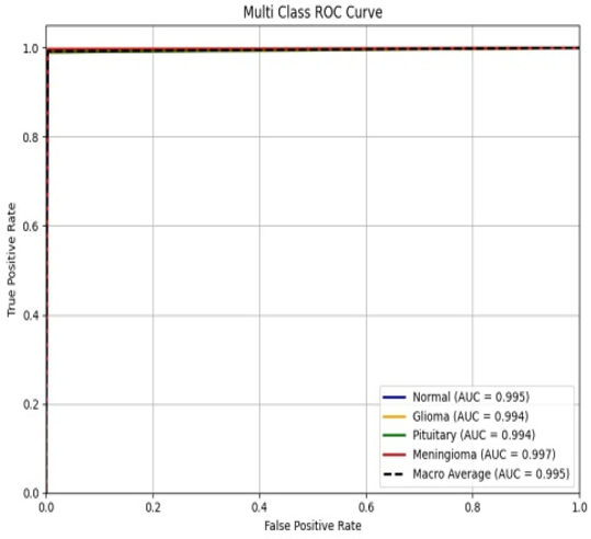
Figure 8 shows the Receiver Operating Characteristic (ROC) plot of the 8D directional Configuration of Level 3. The multi-class ROC curve [26] demonstrates the strong discriminative capability of the proposed model across all four categories: Normal, Glioma, Pituitary, and Meningioma. The curves for each class closely approach the top-left corner of the plot, indicating high true positive rates with very low false positive rates. The Area Under the Curve (AUC) values are exceptionally high, with 0.995 for Normal, 0.994 for Glioma, 0.994 for Pituitary, and 0.997 for Meningioma. The macro-average AUC of 0.995 further confirms that the model maintains balanced and consistent performance across all classes. Figure 8 presents the multiclass ROC curves with AUC values close to 1.0 for all classes, confirming the superior discriminative capability and classification reliability of the proposed work. Overall, the ROC analysis highlights the model’s near-perfect classification ability and its effectiveness in accurately distinguishing between different types of brain tumors.
Figure 8. Receiver Operating Characteristic (ROC) plot of 8D directional configuration of level 3
This work focuses on developing a hybrid deep learning and geometric multiscale framework for the classification of brain tumors by using MRI images. It uses a Bendlet transform to integrate U-Net based segmentation and curvature sensitive feature extraction in a pipeline, which can be followed by feature optimization via whale optimization algorithm and final classification with a fully connected neural network.
The analyzed performance of various directional parameters (2D, 4D, 8D, 16D & 32D) and decomposition levels (level 1-4) shows that the increasing directional parameters upgrade feature discrimination up to better configurations. Especially, it demonstrates the highest performance with 8 directional decomposition at level 3, the values of accuracy, sensitivity, and specificity are 99.21%, 98.81%, and 99.39%, respectively. Therefore, this configuration balances multiscale detail preservation and curvature representations. But Marginal performance degradation provides possible feature redundancy.
The proposed method demonstrates that the integration of curvature-aware representation with Bendlet transformation improves boundary characterization and classification accuracy of tumors. This provides a framework for medical imaging and analysis, especially where the irregular boundaries and structural curvature play a vital role. Future works can focus on integrating the bendlet coefficient into end-to-end deep architecture to improve performance and computational efficiency further.
[1] Musallam, A.S., Sherif, A.S., Hussein, M.K. (2022). A new convolutional neural network architecture for automatic detection of brain tumors in magnetic resonance imaging images. IEEE Access, 10: 2775-2782. https://doi.org/10.1109/ACCESS.2022.3140289
[2] Mithun, M.S., Joseph Jawhar, S.J. (2024). Detection and classification on MRI images of brain tumor using YOLO NAS deep learning model. Journal of Radiation Research and Applied Sciences, 17(4): 101113. https://doi.org/10.1016/j.jrras.2024.101113
[3] Poovizhi, S., Ganesh Babu, T.R. (2020). An efficient skin cancer diagnostic system using bendlet transform and support vector machine. Anais da Academia Brasileira de Ciências, 92: e20190554. https://doi.org/10.1590/0001-3765202020190554
[4] Elazab, N., Gab Allah, W.A., Elmogy, M. (2024). A multi class brain tumor grading system based on histopathological images using a hybrid YOLO and RESNET networks. Scientific Reports, 14: 4584. https://doi.org/10.1038/s41598-024-54864-6
[5] Kurt Pehlivanoğlu, M., İnce, İ., Kından, B.A., Eker, A.G., Doğan, İ. (2025). Towards advanced brain tumor segmentation: A novel hybrid architecture integrating UNet, FCN & YOLO models on the newly introduced BTS-DS 2024 dataset. European Physical Journal, 234(15): 4421-4435. https://doi.org/10.1140/epjs/s11734-025-01698-6
[6] Ahmad, S., Choudhury, P.K. (2022). On the performance of deep transfer learning networks for brain tumor detection using MR images. IEEE Access, 10: 59099-59114. https://doi.org/10.1109/ACCESS.2022.3179376
[7] Sharma, A.K., Nandal, A., Dhaka, A., et al. (2023). Brain tumor classification using the modified ResNet50 model based on transfer learning. Biomedical Signal Processing and Control, 86: 105299. https://doi.org/10.1016/j.bspc.2023.105299
[8] Sun, H., Yang, S., Chen, L., et al. (2023). Brain tumor image segmentation based on improved FPN. BMC Medical Imaging, 23(1): 172. https://doi.org/10.1186/s12880-023-01131-1
[9] Allah, A.M.G., Sarhan, A.M., Elshennawy, N.M. (2023). Edge U-net: Brain tumor segmentation using MRI based on deep U-Net model with boundary information. Expert Systems with Applications, 213: 118833. https://doi.org/10.1016/j.eswa.2022.118833
[10] Praveena, R., Ganesh Babu, T.R., Suvetha, S., Swetha, S., Tamilarasan, G. (2024). Semantic segmentation of lungs using U-Net. Journal of Innovative Image Processing, 6(2): 154-163. https://doi.org/10.36548/jiip.2024.2.006
[11] Krishnapriya, S., Karuna, Y. (2024). A deep learning model for the localization and extraction of brain tumors from MR images using YOLOv7 and grab cut algorithm. Frontiers in Oncology, 14: 1347363. https://doi.org/10.3389/fonc.2024.1347363
[12] Naser, M.A., Deen, M.J. (2020). Brain tumor segmentation and grading of lower grade glioma using deep learning in MRI images. Computers in Biology and Medicine, 121: 103758. https://doi.org/10.1016/j.compbiomed.2020.103758
[13] Shafi, A.S.M., Rahman, M.B., Anwar, T., Halder, R.S., Kays, H.M.E. (2021). Classification of brain tumors and auto-immune disease using ensemble learning. Informatics in Medicine Unlocked, 24: 100608. https://doi.org/10.1016/j.imu.2021.100608
[14] Masood, M., Nazir, T., Nawaz, M., et al. (2021). A novel deep learning method for recognition and classification of brain tumors from MRI images. Diagnostics, 11(5): 744. https://doi.org/10.3390/diagnostics11050744
[15] Badjie, B., Ulker, E.D. (2022). A deep transfer learning based architecture for brain tumor classification using MR images. Information Technology and Control, 51(2): 332-344. https://doi.org/10.5755/j01.itc.51.2.30835
[16] Vankdothu, R., Hameed, M.A. (2022). Brain tumor segmentation of MR images using SVM and fuzzy classifier in machine learning. Measurement: Sensors, 24: 100440. https://doi.org/10.1016/j.measen.2022.100440
[17] Raghuram, B., Hanumanthu, B. (2023). Brain tumor image identification and classification on the internet of medical things using deep learning. Measurement: Sensors, 30: 100905. https://doi.org/10.1016/j.measen.2023.100905
[18] Jiang, S., Gu, Y., Kumar, E. (2023). Magnetic resonance imaging (MRI) brain tumor image classification based on five machine learning algorithms. Cloud Computing and Data Science, 122-133. https://doi.org/10.37256/ccds.4220232740
[19] Kalaiselvi, S., Thailambal, G. (2024). Brain tumor diagnosis from MR images using boosted multi-gradient support vector machine classifier. Measurement: Sensors, 32: 101071. https://doi.org/10.1016/j.measen.2024.101071
[20] Alqudah, A.M., Alquraan, H., Abu Qasmieh, I., Alqudah, A., Al-Sharu, W. (2019). Brain tumor classification using deep learning technique-a comparison between cropped, uncropped & segmented lesion images with different sizes. International Journal of Advanced Trends in Computer Science and Engineering, 8(6): 3684-3691. https://doi.org/10.48550/arXiv.2001.08844
[21] Irmak, E. (2021). Multi-classification of brain tumor MRI images using deep convolutional neural network with fully optimized framework. Iranian Journal of Science and Technology, Transactions of Electrical Engineering, 45(3): 1015-1036. https://doi.org/10.1007/s40998-021-00426-9
[22] Elango, S., Praveena, R., Karthik, G.L., Sakthi, S., gansala, A., Navaneethakrishnan, S.R. (2025). Automated grading of diabetic retinopathy using stacked DR-CNN: A deep learning approach. In IEEE International Conference on Smart Structures and Systems, Chennai, India, pp. 1-6. https://doi.org/10.1109/ICSSS66939.2025.11346326
[23] R., R., T., B.R., Reddy, E.G., D., P., C., J., T.R., G.B. (2025). Deep belief networks for multi-class brain tumor classification with improved diagnostic accuracy. Journal of Innovative Image Processing, 7(1): 97-118. https://doi.org/10.36548/jiip.2025.1.005
[24] Poovizhi, S., Babu, T.G., Praveena, R. (2021). Certain investigations on melanoma detection using non-subsampled bendlet transform with different classifiers. Molecular & Cellular Biomechanics, 18(4): 201. https://doi.org/ 10.32604/mcb.2021.017984
[25] Mzoughi, H., Njeh, I., Wali, A., Slima, M.B., BenHamida, A., Mhiri, C. (2020). Deep multi-scale 3D convolutional neural network (CNN) for MRI gliomas brain tumor classification. Journal of Digital Imaging, 33(4): 903-915. https://doi.org/10.1007/s10278-020-00347-9
[26] Sriram, G., Praveena, R. (2024). Design of a predictive modeling system for MRI brain image classification. Traitement du Signal, 41: 3265. https://doi.org/10.18280/ts.410642