Kavitha Marimuthu | Senthilkumar Selvaraj* | Palani Murugan Selvam | Sivakumar Sathasivam
© 2026 The authors. This article is published by IIETA and is licensed under the CC BY 4.0 license (http://creativecommons.org/licenses/by/4.0/).
OPEN ACCESS
Histopathology image analysis has become an essential diagnostic tool in the early detection of cancer, enabling precise identification of malignant regions from stained tissue slides. These high-resolution microscopic images show details at the cellular level, but they are hard to read because of tissue irregularities, overlapping nuclei, color differences, and structural heterogeneity. Traditional computational methods are primarily based on convolutional neural networks (CNNs), transformers, and graph-based models, which often struggle to retain spatial hierarchies, interpret pose variations of cellular entities, and handle uncertain predictions, especially in borderline malignancies. To address these limitations, this research proposes a novel architecture, the Self-Predictive Attention and Recursive Capsule Synthesis Network (SPARCS-Net), which is designed to emulate biologically consistent decision-making through recursive capsule-based learning. The network simulates cellular orientation and spatial dynamics without using convolutional filters or graph topologies. It does this by adding self-predictive feedback and multi-scale spatial voting to make classification more reliable. Experiments were conducted using the benchmark Kaggle Histopathologic Cancer Detection dataset consisting of 220,025 image patches. The proposed model achieved a classification accuracy of 96.74%, an AUC of 0.981, a precision of 95.10%, a recall of 96.30%, and an F1-score of 95.69%, outperforming baseline models such as ResNet50 and ViT by 3–5% across all key metrics. These results affirm SPARCS-Net’s capability to deliver precise, interpretable, and biologically aligned cancer detection in histopathological workflows.
oral lesion segmentation, histopathological image classification, Self-Predictive Attention and Recursive Capsule Synthesis Network architecture, tissue morphology mapping, deep feature enhancement, tumor region recognition, multi-scale convolution layers, attention fusion strategy
Histopathology serves as the definitive diagnostic standard for a wide range of cancers by enabling cellular-level observation of tissue specimens stained using hematoxylin and eosin techniques [1, 2]. The digitization of these stained slides has ushered in the era of computational histopathology, where image analysis techniques can assist or automate diagnostic interpretations. These digitized histological images contain a wealth of morphological, textural, and color-based information that reflects key cellular features such as nuclear pleomorphism, mitotic activity, and tissue architecture. Unlike radiological images, which operate at macroscopic resolutions, histopathological images reveal microscopic shades critical for assessing malignancy [3]. These images often reach resolutions exceeding several thousand pixels per dimension, allowing observation of individual nuclei, cell boundaries, and stroma. This granularity supports applications such as tumor grading, cancer subtype identification, and biomarker quantification. Furthermore, the patch-wise structure of scanned whole-slide images enables localized assessment of tissue health, making histopathology particularly suitable for computer-assisted diagnosis. Advanced image analysis can also support pathologists by highlighting suspicious regions, reducing manual fatigue, and enabling second-opinion systems in clinical workflows. With an increasing number of hospitals adopting digital pathology systems, there is a growing demand for computational models that can process, interpret, and extract meaningful patterns from these high-dimensional image sets to assist in robust cancer diagnosis and prognosis.
Despite its central role in diagnostic pathology, the analysis of histopathological images presents significant operational and methodological challenges. One of the primary obstacles lies in the inherent variability of tissue samples, stemming from differences in slide preparation, staining intensity, and inter-laboratory protocols. Such inconsistencies can cause significant shifts in image texture and color, leading to reduced generalizability of learned features across datasets. Additionally, histopathological images often contain large areas of non-informative background, fibrous tissue, or blood cells, which can confuse automated systems not trained to discriminate tissue-rich regions. Manual annotation of cancerous regions requires domain expertise and is time-consuming, leading to limited availability of precisely labeled data for supervised learning approaches. Moreover, the high resolution of whole-slide images necessitates subdivision into small patches for processing, causing potential loss of global context. Interpretability also remains a critical concern, as many automated systems fail to provide region-wise rationale for their decisions, hindering clinical trust. Models based solely on pixel-level features may not adequately capture structural information such as glandular arrangements or nuclear alignment, which are often essential for cancer grading. These practical limitations demand architectural innovations that can account for spatial relationships, manage data uncertainty, and adapt to the biological heterogeneity characteristic of cancerous tissues in a clinically acceptable manner.
A considerable volume of research has focused on convolutional neural networks (CNNs) as the primary framework for histopathological image classification and detection [4-6]. CNNs offer hierarchical feature extraction capabilities that can model local textures, edges, and color distributions effectively. Early models utilized standard architectures such as VGG16 and ResNet, fine-tuned on histopathology datasets to identify cancerous tissue regions [7-9]. These models typically operate on fixed-size patches cropped from whole-slide images and rely on sliding window inference to predict tissue health. While CNNs have demonstrated respectable classification accuracy, their kernel-based operations are inherently limited to learning localized patterns and often require large receptive fields or deeper networks to capture long-range dependencies. This limitation becomes more evident in images where cellular arrangement or inter-nuclear spacing carries diagnostic relevance. Moreover, CNNs are sensitive to spatial distortions and may underperform when faced with scale, orientation, or stain variability. Recently, self-attention-based architectures such as Vision Transformers (ViT) have emerged as an alternative to convolutional models [10]. Transformers capture global contextual information using position-aware tokenization and attention weights. In histopathology, ViT variants have been adapted to model long-range tissue interactions and achieve state-of-the-art results on several cancer classification benchmarks. However, their tokenization process often assumes grid-based uniformity, which may not align well with the irregular and heterogeneous nature of histopathological structures.
Alongside convolutional and transformer-based strategies, other researchers have explored graph neural networks (GNNs) and multiple instance learning (MIL) frameworks to better encode the spatial complexity inherent in histopathological imagery. GNN-based methods typically represent nuclei or cell clusters as graph nodes, with edges capturing spatial proximity or feature similarity [11]. These approaches aim to model cellular microenvironments and local interactions critical to understanding malignancy progression. Although effective for node-level or region-based predictions, such models require explicit cell segmentation and graph construction, which can be computationally expensive and sensitive to segmentation errors. Meanwhile, MIL-based approaches consider the entire slide as a bag of instances (patches) and learn to predict slide-level labels using weak supervision. While suitable for large-scale datasets with limited annotations, MIL models often suffer from information dilution and lack fine-grained decision mechanisms. The limitations across these categories—convolution’s restricted context, transformer’s rigid tokenization, graph reliance on segmentation, and MIL’s weak supervision—highlight a pressing need for architectures that can preserve spatial detail, adapt to irregular cellular layouts, and offer robust confidence-aware outputs. Motivated by these gaps, the present study seeks to develop a biologically grounded, spatially aware, and self-refining architecture that can accurately interpret patch-wise histopathological features and provide explainable cancer predictions without relying on traditional deep learning constraints.
To overcome the challenges outlined above, this research introduces a novel Self-Predictive Attention and Recursive Capsule Synthesis Network (SPARCS-Net) specifically designed for patch-wise classification in histopathological cancer detection. The model diverges from traditional CNNs and transformers by utilizing capsule networks that maintain pose, orientation, and structural hierarchies of cellular elements. Unlike scalar activations used in convolutional filters, SPARCS-Net employs vector-based capsules that encapsulate complex tissue characteristics such as shape deformation and spatial alignment. A key novelty lies in the recursive refinement mechanism, wherein capsule representations are iteratively updated through feedback loops, emulating how pathologists re-evaluate tissue regions during diagnosis. Additionally, the network incorporates a self-predictive attention block that estimates its own confidence in feature extraction, allowing dynamic suppression of uncertain activations. The multi-scale spatial voting scheme enhances robustness by integrating predictions across varying resolutions. Unlike existing methods, SPARCS-Net does not depend on segmentation masks, bag-level labels, or graph construction. It offers a complete decision pipeline from patch-level processing to slide-level agreement synthesis. The architectural design enables high accuracy in cancer detection, while maintaining interpretability through capsule agreement maps. This makes the model not only suitable for automated classification but also for clinical decision support systems requiring spatial reasoning and visual traceability. The major contributions of the research work are presented as follows.
•Proposed a capsule-based architecture SPARCS-Net for histopathology image processing. The proposed model includes a recursive capsule refinement mechanism for dynamic spatial representation and decision enhancement. In addition, a self-predictive attention block is included, which evaluates and suppresses low-confidence feature activations during inference. Finally, a multi-scale spatial voting strategy is incorporated to synthesize predictions from variable patch resolutions.
•Presented a detailed experimental analysis using a benchmark histopathologic cancer detection dataset and demonstrated the superior performance with conventional deep learning models.
The remaining discussions in the article are arranged as follows. Recent research works on histopathological cancer detection are analyzed, and their merits and demerits are summarized as a literature review in section 2. The proposed model is presented in detail in section 3, and the experimental results and discussion are presented in section 4. Finally, the research work conclusion is presented in section 5.
Numerous deep learning-based strategies have been investigated for oral cancer detection using histopathological and clinical imagery. These approaches range from traditional convolutional models to advanced hybrid architectures integrating attention mechanisms, feature fusion, and transfer learning. Several methods emphasize improved classification accuracy, robustness to limited datasets, and enhanced diagnostic reliability. Despite notable advancements, current systems face constraints in generalization, interpretability, and adaptability to clinical conditions, necessitating more refined models tailored for precise and early-stage oral malignancy diagnosis.
The oral cancer classification model presented evaluates CNNs, transformer networks, and few-shot learning models such as Siamese, Triplet, and ProtoNet for detecting dysplasia and oral squamous cell carcinoma (OSCC) [12]. The experimentation reveals the DenseNet-121 model, which achieved the highest balanced accuracy which is outperforming transformer variants. Few-shot models underperformed, with results significantly impacted by configuration and optimizer choice. While the study highlights model performance under limited data scenarios, it is constrained by optimizer sensitivity and lacks interpretability or clinical validation necessary for practical deployment in diagnostic workflows.
The DeepPatchNet model presented integrates DeepLabV3+ with ConvMixer to form a compact and interpretable model for histopathological image classification, particularly targeting OSCC detection [13]. Evaluated on the NDB-UFES and an independent OSCC dataset, the model outperformed existing architectures including ViT, ConvNeXt, and InceptionResNetV2, achieving better accuracy and closely aligned scores across precision, recall, and F1 metrics. A key strength lies in the incorporation of Grad-CAM for visual justification, supporting clinical interpretability. However, the model’s generalizability remains uncertain due to limited external validation, and the performance gap with ensemble or hybrid models indicates potential for further enhancement.
The deep learning-based classification model presented incorporates two deep learning architectures tailored for accurate segmentation and classification of OSCC from histopathological images [14]. MaskMeanShiftCNN utilizes color, texture, and shape-based cues for precise tumor region segmentation, while SV-OnionNet focuses on early-stage OSCC identification using spatially variant features. Experimental analysis reports high classification accuracy and sensitivity, indicating robust detection performance. Despite their effectiveness, the study does not address model generalization across datasets with varying stain protocols or imaging artifacts, and lacks interpretability features critical for real-time integration into clinical diagnostic systems.
The application of YOLOv5 object detection is presented for identifying OSCC lesions from intraoral clinical images [15]. Using a dataset of 65 annotated cases verified by experts, the model was trained and evaluated through a confusion matrix-based analysis. On the test set, YOLOv5 achieved better F1-score, sensitivity, and precision values, reflecting moderate detection capability. The findings affirm that OSCC lesions present discernible visual markers suitable for detection; however, the limited dataset size and lack of image diversity constrain model generalization and performance, emphasizing the need for larger, more varied datasets for improved diagnostic accuracy.
The deep learning model reported for histopathological classification of breast, colon, and lung cancers utilizes both low-level and high-level image features [16]. Evaluated on benchmark datasets, the presented model achieved exceptional accuracy. To enhance transparency, Local Interpretable Model-Agnostic Explanations (LIME) and SHapley Additive exPlanations (SHAP) were incorporated for explainability, enabling visual interpretation of prediction rationale. A parameter sensitivity analysis was also performed to assess model robustness. Despite high performance, the model's reliance on predefined feature levels and dataset-specific tuning may restrict adaptability across diverse pathological conditions and unseen imaging modalities.
A modified prototypical network model is presented for oral cancer detection that addresses data scarcity through few-shot learning [17]. Unlike standard models, it employs dual feature extractors to independently process prototype and query samples, enhancing feature discrimination. A customized loss function further improves class separation and robustness. Experimental validation on histopathological datasets confirms the model's superior classification accuracy compared to conventional baselines. While the architecture effectively mitigates the dependency on large training sets, it may still face challenges in capturing complex spatial patterns present in highly heterogeneous tissue structures and lacks interpretability modules required for clinical trust and adoption in diagnostic workflows.
A detailed evaluation of multiple CNN architectures is reported for oral classification [18]. Deep learning models like VGG16, ResNet50, LeNet-5, MobileNetV2, and Inception V3 were used to classify oral cavity squamous cell carcinoma and dysplasia from virtual slide images. Using NEOR and OCSCC datasets, image tiles were categorized as normal or malignant, with MobileNetV2 yielding the better accuracy. Evaluation based on accuracy, precision, recall, F1-score, and AUC enabled comparative assessment across models. While the results affirm CNNs' reliability for early diagnosis, the study lacks interpretability mechanisms and does not explore model robustness under staining variability, which limits immediate clinical adoption in diverse real-world settings.
A multimodal diagnostic approach presented integrates histopathological images with demographic and clinical data for improved detection of OSCC and leukoplakia variants [19]. Using the newly curated NDB-UFES dataset of 237 expert-verified samples, the authors evaluate fusion strategies including Concatenation, Mutual Attention, MetaBlock, and MetaNet with modern deep learning backbones. MetaBlock with ResNetV2 achieved the highest balanced accuracy and a significant point gain in complex classification tasks. Despite its strength in performance enhancement, the model’s dependency on structured clinical metadata limits applicability where comprehensive patient information is unavailable or inconsistent.
The strategies presented for classifying OSCC histopathological images incorporate transfer learning with fine-tuned pretrained Deep Convolutional Neural Networks (DCNNs) and a custom deep CNN trained from scratch [20]. Pretrained models such as VGG16, VGG19, ResNet50, InceptionV3, and MobileNet were partially unfrozen to balance feature reuse and training efficiency on a small dataset. Comparative evaluation revealed that ResNet50 achieved better accuracy. While the study highlights the effectiveness of transfer learning in low-data settings, limitations remain in model generalizability and interpretability, with no attention to explainability or adaptability to multiclass clinical conditions.
The deep learning model XceptionAttnV1 presented enhances oral cancer classification by integrating Contrast Limited Adaptive Histogram Equalization (CLAHE)-based contrast enhancement, a custom convolutional layer within Xception’s middle flow, and a channel attention mechanism for focused feature extraction [21]. Designed to distinguish benign from malignant lesions, the model achieves high performance and balanced precision, recall, and F1-scores. Evaluation includes 5-fold cross-validation, analysis of variance (ANOVA), and paired t-tests to ensure statistical reliability. While the approach effectively improves generalization and localization, its dependency on extensive pre-processing and model complexity may affect scalability in real-time clinical workflows or resource-limited diagnostic settings.
The Multi-Layer Visual Feature Fusion (MLVFF) approach presented integrates Local Binary Patterns (LBP) with CNNs to enhance oral cancer detection by enriching feature discrimination [22]. By leveraging both texture-based and deep hierarchical representations, the model achieves better test accuracy and indicates its reliable classification performance. The fusion technique effectively addresses feature insufficiency in early lesion identification. However, the framework lacks attention to model interpretability and does not evaluate robustness under diverse imaging conditions or class imbalance, limiting its adaptability to broader clinical scenarios. The study also outlines future directions to refine cancer diagnostic methodologies.
The deep learning model presented for detecting skin and oral cancers using medical imagery compares multiple CNN architectures, including AlexNet, VGGNet, Inception, ResNet, DenseNet, and a GNN variant [23]. Image enhancement and filtering are applied for noise reduction, followed by data augmentation to improve model generalization. Performance is assessed using training and validation accuracy and loss metrics, with DenseNet emerging as the top performer on the skin cancer dataset. However, the analysis lacks detailed evaluation on oral cancer images and does not address clinical interpretability or computational cost, which are critical for real-world diagnostic deployment.
A lightweight hybrid architecture presented merges CNNs for local pattern extraction with Transformer attention for global context modeling, aiming to enhance oral disease diagnosis across clinical and histopathological images [24]. Evaluated on three diverse datasets, the model achieved better outperforming several existing methods while maintaining computational efficiency. Its low parameter count and reduced inference latency make it suitable for deployment in mobile and resource-limited settings. Despite strong performance, the approach may face constraints in complex multi-class classification tasks and lacks domain-specific customization for complex tissue-level diagnostic variability across patient populations.
The hybrid deep learning model presented combines CNN, Bi-LSTM, and Bi-GRU modules for extracting spatial, contextual, and sequential features from histopathological oral cancer images [25]. These deep features are fused and classified using a soft-voting ensemble comprising five baseline classifiers such as LR, DT, k-NN, SVM, and SGD to enhance prediction reliability. The model is evaluated on two standard datasets, HOCDD and HRNEOCD, achieving better accuracies, which clearly demonstrates the high predictive strength. However, the approach relies on handpicked ensemble components without adaptive weighting and lacks interpretability mechanisms for clinical validation or spatial explanation of malignancies.
A hybrid deep learning architecture presented for histopathology image classification fuses global and local features through a serial hierarchical structure [26]. The model incorporates an Internal Communication Hierarchical Fusion Block (ICHF) and an Efficient Dual Self-Attention (EDA) mechanism to enhance semantic richness and maintain feature consistency. Evaluated on four benchmark datasets with added Gaussian noise, Internal Communication Network with Dual Self-Attention (ICDNET) demonstrated strong accuracy and resilience under limited training data, highlighting its clinical potential. However, the model’s complexity may hinder deployment in low-resource environments, and its performance across diverse staining protocols or rare pathological variants remains untested.
The reviewed techniques show a lot of advancement in oral cancer image classification, but their architecture is fundamentally different from the spatial nature of the histopathological diagnosis. CNN-based models typically rely on local receptive fields to learn scalar feature responses, which proves highly effective for texture and edge extraction, but may result in loss of information about parts and whole, pose, and orientation between the nuclei, cytoplasm, epithelial structures, and stromal regions. Transformer-based models have been designed to enhance the modeling of context by self-attention, but the use of fixed tokens obtained from image patches can decrease fine cellular continuity and does not explicitly support modeling of morphological hierarchy. While graph-based methods can be used to capture spatial relationships between the cellular components, they are sensitive to inaccuracies in cell segmentation and graph construction. In the same way, ensemble and transfer learning models boost classification accuracy but typically offer little insight into the contribution of spatial tissue organization to the classification. SPARCS-Net, on the other hand, aims to maintain cellular architecture using the vector representation of capsules, whose output represents both the presence of the feature and its spatial configuration. Recursive refinement increases agreement of consistent tissue structures, and self-predictive attention decreases responses of uncertain capsules. Thus, the proposed model is a conceptually different model where the classification is not only based on feature strength but also on the spatial agreement, confidence estimation, and multi-scale morphological voting.
The literature overview presented in Table 1 confirms that the existing deep learning models have made remarkable advancements in oral cancer diagnosis; however, the majority of the existing models lack some aspects of providing adequate cell spatial hierarchy preservation in the direction and interpretability in the decision-making process. Thus, besides classification accuracy, the main research gap is related to the ability to preserve morphological relations between the histopathological structures and to explain the reliability of prediction of a model. At first, deep learning models exhibit notable progress in oral cancer diagnosis, several critical gaps persist across the reviewed works. Many approaches rely heavily on CNN backbones or simple ensemble strategies, which, although effective for feature extraction, often struggle with spatial context preservation, especially in histopathological images where cellular arrangements and morphological hierarchies carry diagnostic value. Transformer-based and few-shot learning models offer potential for contextual awareness and low-data adaptability, yet they either face computational inefficiencies or yield inconsistent performance due to sensitivity in architecture and optimizer choices. While some models integrate attention mechanisms or perform feature-level fusion, interpretability remains underexplored, with limited deployment of explainable modules to visualize and validate learned representations. Several studies demonstrate high accuracy using curated or moderately sized datasets, yet lack robustness analysis under variable staining, noise, and real-world clinical diversity. Hybrid models incorporating both clinical metadata and image data exist but are dataset-dependent and rarely generalizable across tasks involving oral dysplasia and carcinoma differentiation. Additionally, lightweight models suitable for constrained environments often sacrifice diagnostic depth. These limitations collectively highlight the need for a biologically aligned, explainable, spatially aware, and computationally efficient diagnostic model that can generalize across imaging conditions and support both interpretability and practical clinical integration.
Table 1. Literature review summary
|
Ref. |
Methodology |
Merit |
Limitation |
|
[12] |
Comparative evaluation of CNNs, transformers, and few-shot learning on P-NDB-UFES dataset |
DenseNet-121 outperformed with balanced accuracy and recall |
Optimizer sensitivity affected few-shot learning performance |
|
[13] |
DeepPatchNet combining DeepLabV3+ and ConvMixer with Grad-CAM |
Superior accuracy with built-in visualization for feature interpretability |
Requires further validation across clinical datasets |
|
[14] |
Dual models—MaskMeanShiftCNN and SV-OnionNet—for segmentation and classification |
Reached 99% accuracy and sensitivity on OSCC detection |
Absence of external data validation and real-time interpretability |
|
[15] |
YOLOv5 object detection on intraoral cancer lesion dataset |
Showcased feasibility of direct lesion localization using deep models |
Limited dataset and moderate performance metrics |
|
[16] |
Cancer diagnosis model using LIME and SHAP with BreakHis and LC25000 datasets |
Integrated explainability tools with strong accuracy across datasets |
Requires fine-tuning for each cancer type and lacks class diversity |
|
[17] |
Modified prototypical network with dual feature extractors and customized loss |
Effectively minimized training data requirement |
Spatial complexity handling remains limited |
|
[18] |
CNN-based classification using MobileNetV2, ResNet50, and VGG on NEOR, OCSCC |
MobileNetV2 achieved the highest accuracy for OSCC identification |
Lacks explainability and generalization testing across datasets |
|
[19] |
Fusion of histopathological images with clinical data using MetaBlock and ResNetV2 |
Improved classification performance through multimodal integration |
Inapplicability in settings lacking structured patient metadata |
|
[20] |
Transfer learning with fine-tuned DCNNs and baseline CNN trained from scratch |
ResNet50 outperformed all models with balanced metrics |
Does not incorporate model interpretability or multi-class classification |
|
[21] |
XceptionAttnV1 using CLAHE and attention-enhanced convolutional blocks |
Achieved strong classification scores with statistical validation |
Heavy reliance on preprocessing and complex structure |
|
[22] |
Multi-Layer Visual Feature Fusion combining LBP and CNN layers |
Enhanced feature discrimination and high test accuracy |
Did not address model transparency or image variability |
|
[23] |
Comparative study of CNNs and GNNs on skin and oral cancer datasets |
DenseNet performed well under preprocessed and augmented data |
Lack of detailed analysis for oral cancer and limited clinical insight |
|
[8] |
CNN-Transformer hybrid for MOD and OC detection with reduced FLOPs |
Lightweight, efficient, and suited for resource-limited scenarios |
Lower accuracy for complex histopathology datasets |
|
[1] |
Ensemble of CNN, Bi-LSTM, and Bi-GRU with soft-voting classifiers |
Achieved high classification accuracy across multiple datasets |
No adaptive weight tuning and lacks interpretability support |
|
[12] |
ICDNET model with ICHF and EDA for global-local feature fusion |
Demonstrated noise resilience and semantic preservation |
Complex architecture with high implementation cost |
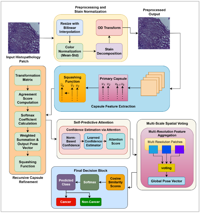
The proposed research introduces a novel architectural SPARCS-Net for patch-level classification of histopathological images used in cancer detection. This model is specifically constructed using capsule networks due to their inherent ability to preserve spatial pose, orientation, and morphological hierarchies of cellular structures, where the key factors are often lost in conventional convolutional models. Unlike scalar activations used in standard networks, capsules encode vector representations that retain spatial dynamics, enabling a more biologically accurate interpretation of tissue architecture. The recursive refinement incorporated into SPARCS-Net allows iterative improvement of capsule representations through feedback loops, mimicking the re-evaluation strategy used by human pathologists when analyzing complex tissue regions. Additionally, a self-predictive attention mechanism is embedded within the model to evaluate the certainty of extracted features and suppress those with low confidence, thereby strengthening the reliability of predictions. As illustrated in Figure 1, the complete process begins with preprocessing of raw histopathological image patches extracted from the Kaggle dataset. Preprocessing involves stain normalization to reduce color variance and patch filtering to eliminate background regions. These patches are then input into the capsule feature extraction module, which generates pose vectors for various morphological elements. The recursive capsule block subsequently refines these vectors across multiple iterations, improving feature clarity and spatial alignment. In parallel, the self-predictive attention unit computes reliability scores for each capsule output, guiding the network to prioritize trustworthy features. The refined outputs are passed through a multi-scale spatial voting mechanism, where predictions at different resolutions are fused to accommodate diverse tissue structures. Finally, the agreement score classifier evaluates the collective output using vector-based consistency, producing both the cancer prediction and a corresponding spatial map highlighting regions of diagnostic importance. This process ensures accurate, explainable, and structurally consistent cancer detection from histopathological imagery.
Figure 1. Proposed model overview
3.1 Input image acquisition
In digital histopathology, each raw tissue image is obtained as a high-resolution color image. The image patch is mathematically modeled as a 3-dimensional tensor of intensity values defined over spatial and spectral dimensions. Let an input patch be represented as $\mathrm{I}(u, v, c) \in R^{H \times W \times 3}$ in which $u \in\{1,2, \ldots, \mathrm{H}\}$ represents the pixel row index (height), $v \in\{1,2, \ldots, \mathrm{~W}\}$ represents the pixel column index (width), $c \in\{1,2,3\}$ denotes the color channel (Red, Green, Blue). Each element $\mathrm{I}(u, v, c)$ holds an integer value in the range [0,255], corresponding to the pixel intensity of the respective color channel. The full image dataset is denoted as a collection of labeled tuples, which is mathematically represented as:
$D=\left\{\left(I_i, y_i\right) \mid i=1,2, \ldots, N\right\}$ (1)
where, $\mathrm{I}_i$ is the $i$-th image patch, $y_i \in\{0,1\}$ is the class label for that patch, $N$ is the total number of patches extracted. To ensure uniformity in dimensions, each image is resized to a fixed target resolution using bilinear interpolation. This operation generates a new patch $\widehat{\mathrm{I}}_i \in R^{H_0 \times W_0 \times 3}$, where,
$\hat{\mathrm{I}}_i\left(u^{\prime}, v^{\prime}, c\right)=\sum_{m=0}^1 \sum_{n=0}^1 w_{m n} \cdot \mathrm{I}_i\left(u_m, v_n, c\right)$ (2)
where, $u^{\prime}, v^{\prime}$ are coordinates in the resized image grid, $u_m, v_n$ are the surrounding pixel coordinates in the original image space, $w_{m n} \in[0,1]$ are bilinear interpolation weights derived from fractional distances. Following resizing, the pixel intensity values are normalized to standardize the input scale. For each color channel, normalization is applied, which is mathematically expressed as:
$\mathrm{I}_i^{\prime \prime}(u, v, c)=\frac{\hat{\mathrm{I}}_i(u, v, c)-\mu_c}{\sigma_c}$ (3)
where, $\mathrm{I}_i^{\text {" }}(u, v, c)$ is the normalized pixel value, $\mu_c$ is the mean intensity of the channel $c$ across all training samples, $\sigma_c$ is the standard deviation of the channel $c$ over the dataset. This standardization ensures that each color channel has zero mean and unit variance, mitigating the effects of staining inconsistencies and illumination variations. The entire dataset is finally arranged into a four-dimensional tensor for batch processing. Mathematically, it is expressed as:
$X=\left[\mathrm{I}_1^{\prime \prime}, \mathrm{I}_2^{\prime \prime}, \ldots, \mathrm{I}_{\mathrm{B}}^{\prime \prime}\right] \in R^{B \times H_0 \times W_0 \times 3}$ (4)
where, $B$ is the batch size, $H_0$ and $W_0$ are the standardized height and width of the patches, and 3 corresponds to the RGB color channels. This tensor preserves both the spatial intensity patterns and the stain characteristics of the original image pixels. As such, $X$ serves as the raw input representation before being fed into the subsequent capsule-based feature extraction module, while the normalized and batch-organized feature maps are processed separately during model training.
3.2 Preprocessing and stain normalization
Following the acquisition and standardization of image dimensions, each histopathological patch undergoes preprocessing to address the inherent variability introduced by staining protocols, slide preparation techniques, and scanner configurations. Hematoxylin and eosin stains, which respectively highlight nuclei and cytoplasm, produce variations in coloration that can interfere with reliable feature extraction. To minimize this inconsistency, a stain normalization procedure is applied to decompose and reconstruct the image based on reference stain matrices. Let a normalized image patch be denoted by $\mathbf{I}_i^{\prime \prime}(u, v, c) \in R^{H_0 \times W_0 \times 3}$, where each channel represents a color plane in the RGB color space. To separate stain components, a logarithmic optical density (OD) transformation is applied to convert pixel intensities into absorbance values.
$O_i(u, v, c)=-\log _{10}\left(\frac{\mathrm{I}_i^{\prime \prime}(u, v, c)+1}{255}\right)$ (5)
In the above equation $O_i(u, v, c)$ is the OD of the pixel at position ($u, v$) in channel $c$. The value 1 is added to avoid logarithmic singularity. The result represents how much light is absorbed by each stain at that location. The next step involves deconvolving the OD space using a stain matrix $S \in R^{3 \times 2}$, which contains column vectors for hematoxylin and eosin absorbance profiles. The deconvolved stain concentration matrix is computed as:
$\mathrm{C}_{\mathrm{i}}(\mathrm{u}, \mathrm{v},:)=\left(\mathrm{S}^{\top} \mathrm{S}\right)^{-1} \mathrm{~S}^{\top} \cdot \mathrm{O}_{\mathrm{i}}(\mathrm{u}, \mathrm{v},:)$ (6)
where, $C_i(u, v,:) \in R^2$ contains the estimated concentration of hematoxylin and eosin at pixel $(u, v)$, $S$ is the stain matrix calibrated from reference tissue images using singular value decomposition or non-negative matrix factorization. Once the stain concentrations are extracted, a reconstruction is performed using a fixed reference stain matrix $S_{\text {ref }} \in R^{3 \times 2}$ that represents ideal staining conditions. The reconstructed OD is obtained as
$\widehat{O}_i(u, v,:)=S_{\text {ref}}\cdot C_i(u, v,:)$ (7)
This reconstruction adjusts the stain contribution of each pixel to match the reference standard. The final image is then converted back into the RGB space by applying the inverse transformation, which is mathematically expressed as:
$\widehat{\mathrm{I}}_i(u, v, c)=255 \cdot \exp \left(-\widehat{O}_i(u, v, c)\right)$ (8)
In this equation $\hat{\mathrm{I}}_i(u, v, c)$ represents the stain-normalized pixel intensity. The exponential operation reverses the logarithmic OD transformation; the multiplication by 255 restores the values to the 8-bit image domain. After stain normalization, irrelevant regions such as background, whitespace, or debris are removed using tissue coverage estimation. A binary tissue mask is generated by converting the image to grayscale and applying an intensity threshold. Mathematically, it is expressed as:
$M_i(u, v)=\left\{\begin{array}{lc}1 & \text { if } \frac{1}{3} \sum_{c=1}^3 \hat{\mathrm{I}}_i(u, v, c)<\theta \\ 0 & \text { otherwise }\end{array}\right.$ (9)
where, $M_i(u, v)$ is the binary tissue mask at position $(u, v), \theta$ is the pixel intensity threshold used to exclude bright, non-tissue regions. The final tissue content is quantified as a ratio of foreground to total pixels, which is mathematically expressed as:
$\psi_i=\frac{1}{H_0 W_0} \sum_{u=1}^{H_0} \sum_{v=1}^{W_0} M_i(u, v)$ (10)
Only patches satisfying $\psi_i \geq \tau$ are retained for further processing, where $\tau \in[0,1]$ is the minimum tissue coverage threshold.
The parameters for preprocessing were chosen after considering the practical image requirements of the histopathology clinical specimens and preliminary validation stability. To preserve compatibility with the capsule feature extraction module and preserve sufficient cellular and tissue-level details for the classification of oral cancer, the size of the input patch is fixed to be 96 × 96 × 3. Recurrent capsule routing was computationally intensive when patch sizes were larger, but smaller patch sizes did not reveal the local structures of the epithelial cells and their arrangement. Hence, 96 × 96 × 3 was chosen as a compromise that offered good resolution while not being too taxing on the computer.
To eliminate patches dominated by bright background, whitespace, or non-informative slide portions, a threshold τ on tissue coverage was used to reject patches. This threshold was determined on a visual assessment of tissue-retained and tissue-rejected samples as well as a test for validation stability in preliminary trials of tissue-retained samples. Low thresholds left many of the background-rich patches, adding intensity patterns that were not informative, while high thresholds resulted in the loss of partially informative tissue regions. Therefore, the chosen threshold was designed to leave out blank or less informative areas and preserve areas with tissue information.
To minimize color variation due to variation in intensity of H&E staining, slide preparation, and illumination by the scanner, the stain normalization reference matrix was selected. The OD transformation was employed as a method for separating the contributions of hematoxylin and eosin stains from one another, as well as separating the two from direct RGB normalization. The OD transformation was employed because it separated hematoxylin and eosin stain contributions more effectively than direct RGB normalization and also separated the two stains. This helped to maintain the nuclear and cytoplasmic color representation to be consistent before the spatial feature extraction in the capsules. So, the pre-processing selection wasn't a random selection of mathematical options, but was chosen for enhancing tissue relevance, color stability, and model convergence.
This preprocessing stage ensures that only visually informative, stain-normalized image patches are passed to the capsule feature extraction stage, eliminating background noise and standardizing color variation across all histopathological samples.
3.3 Capsule feature extraction
Following preprocessing and stain normalization, each histopathology patch is forwarded into the capsule feature extraction stage. Unlike conventional methods that rely on scalar feature maps generated by convolutional filters, capsule networks represent features as pose vectors. Each vector captures both the presence and spatial attributes of local structures such as nuclei, cytoplasm, or tissue boundaries. This property makes capsules particularly suitable for modeling the geometric variability and orientation diversity present in cancerous tissue sections. Let $\hat{\mathrm{I}}_i(u, v, c) \in R^{H_0 \times W_0 \times 3}$ be the preprocessed and stain-normalized input image patch. The first operation is a standard convolutional projection that transforms the input image into low-level feature maps. This step is mathematically expressed as:
$\begin{gathered}\mathrm{F}_i(m, n, f)=\sum_{a=1}^k \sum_{b=1}^k \sum_{c=1}^3 \widehat{\mathrm{I}}_i(m+a, n+b, c) \cdot W_1(a, b, c, f)+b_1(f)\end{gathered}$ (11)
where, $\mathrm{F}_i(m, n, f)$ is the feature map at spatial position $(m, n)$ for filter $f$, $k$ is the size of the convolutional kernel, $W_1(a, b, c, f)$ is the weight of the kernel at location $(a, b)$ in channel $c$ for filter $f$, $b_1(f)$ is the bias associated with filter $f$, $f \in\{1,2, \ldots, \mathrm{~F}\}$ is the index of the feature channel. The result is a 3D tensor $\mathrm{F}_i \in R^{H_1 \times W_1 \times F}$, which contains scalar activations encoding textural properties of the input patch. To convert these scalar activations into vector representations, the feature tensor is partitioned into groups, each forming a primary capsule. Let the number of primary capsules be $M$, and each capsule outputs a $d$-dimensional vector. The primary capsule matrix is then mathematically expressed as:
$u_j=\operatorname{resh}\operatorname{ape}\left(\mathrm{F}_i[j]\right) \in R^d$ (12)
where, $\mathrm{F}_i[j]$ is the slice of the feature tensor assigned to capsule $j$, $u_j$ is the initial pose vector for capsule $j, d$ is the dimensionality of the pose vector, $j \in\{1,2, \ldots, \mathrm{M}\}$ is the capsule index. These initial vectors undergo a squashing transformation to ensure their magnitude remains between zero and one, preserving the interpretation of length as confidence. Mathematically, it is expressed as:
$p_j=\frac{\left|u_j\right|^2}{1+\left|u_j\right|^2} \cdot \frac{u_j}{\left|u_j\right|}$ (13)
where, $p_j$ is the squashed pose vector for capsule $j$, $\left|u_j\right|$ is the Euclidean norm (length) of the vector, The operation rescales the vector while maintaining its orientation. To prepare for dynamic routing in the next step, each capsule's output is projected into a set of prediction vectors targeting higher-level capsules. The prediction from capsule $j$ to class capsule $k$ is computed as:
$\hat{p}_{j k}=W_{j k} \cdot p_j$ (14)
where, $\hat{p}_{j k} \in R^\acute{d}$ is the prediction vector from capsule $j$ to higher-level capsule $k$, $W_{j k} \in R^{\acute{d} \times d}$ is the transformation matrix learned during training, $\acute{d}$: dimensionality of higher-level pose vectors. At this stage, every capsule contributes multiple prediction vectors aimed at forming higher-level semantic capsules, which will be aggregated through iterative agreement in the next routing phase. The entire capsule feature extraction phase builds a hierarchical spatial representation of the input tissue patch, where local geometric structures are encoded into vectors, and their relationships are mathematically prepared for routing. This ensures the preservation of orientation, location, and presence information, all of which are crucial for distinguishing cancerous and non-cancerous patterns in microscopic tissue images.
3.4 Recursive capsule refinement
Once the primary capsules are constructed and prediction vectors are generated for each higher-level capsule candidate, the network enters a recursive refinement stage. This mechanism is designed to emulate the diagnostic behavior of pathologists who repeatedly observe overlapping or ambiguous regions before finalizing decisions. In the proposed SPARCS-Net, the refinement process is governed by a routing-by-agreement strategy that iteratively improves the precision of capsule outputs based on mutual reinforcement between low-level and high-level capsules. Let each capsule $j \in\{1,2, \ldots, \mathrm{M}\}$ produce a pose vector $p_j \in R^d$, and each target capsule $k \in\{1,2, \ldots, \mathrm{~K}\}$ be formed through agreement among prediction vectors $\hat{p}_{j k} \in R^d$. Each high-level capsule begins with a zero-initialized vector $v_k^{(0)}=0$. The refinement progresses over $T$ routing iterations. At each iteration $t \in\{1, \ldots, \mathrm{~T}\}$, an agreement score is computed between the prediction vector $\hat{p}_{j k}$ and the current state of the capsule $v_k^{(t-1)}$. Mathematically, it is expressed as:
$s_{j k}^{(t)}=\hat{p}_{j k} \cdot v_k^{(t-1)}$ (15)
where, $s_{j k}^{(t)}$ is the scalar similarity score representing alignment between capsule $j$'s prediction and capsule $k$'s current output. These similarity scores are normalized using the softmax function across all target capsules k, yielding routing coefficients. Mathematically, it is expressed as:
$a_{j k}^{(t)}=\frac{\exp \left(s_{j k}^{(t)}\right)}{\sum_{l=1}^K \exp \left(s_{j l}^{(t)}\right)}$ (16)
where, $a_{j k}^{(t)} \in[0,1]$ is the normalized routing weight that determines the contribution of capsule $j$'s prediction to capsule $k$, each source capsule $j$ distributes its influence over all target capsules through $a_{j k}^{(t)}$, ensuring probabilistic routing. The target capsule $k$'s pose vector is then updated as a weighted sum of incoming predictions, which is mathematically expressed as:
$s_k^{(t)}=\sum_{j=1}^M a_{j k}^{(t)} \cdot \hat{p}_{j k}$ (17)
This aggregated vector is passed through a non-linear squashing function to produce the refined pose vector for capsule $k$. Mathematically, it is expressed as:
$v_k^{(t)}=\frac{\left|s_k^{(t)}\right|^2}{1+\left|s_k^{(t)}\right|^2} \cdot \frac{s_k^{(t)}}{\left|s_k^{(t)}\right|}$ (18)
where, $\left|s_k^{(t)}\right|$ is the Euclidean norm of the aggregated vector. The squashing function ensures that the length of the pose vector stays within a unit scale while preserving its direction. This refinement cycle continues for a fixed number of iterations $T$, during which each high-level capsule's output becomes increasingly aligned with consistent predictions from lower capsules. After the final iteration, the output pose vectors $v_k^{(T)}$ serve as the definitive encoded representations of semantic entities (e.g., malignant or benign structures) detected in the image.
3.5 Self-predictive attention confidence estimation
Following the refinement of pose vectors through iterative agreement, the next step is to assess the reliability of each high-level capsule's output. In histopathological tissue classification, certain regions may carry ambiguous features due to poor staining, overlapping cells, or inconsistent morphology. To manage such uncertainty, the proposed SPARCS-Net introduces a self-predictive attention mechanism that computes an internal confidence score for each capsule’s refined output. This mechanism not only highlights trustworthy decisions but also enables the network to suppress unconfident outputs, improving the overall robustness of cancer detection. Let $v_k^{(T)} \in R^\acute{d}$ denote the final pose vector of the $k$-th high-level capsule after $T$ routing iterations. This vector carries semantic information about a structural pattern in the input image. To estimate the confidence of this capsule’s prediction, two complementary strategies are combined: (i) length-based certainty, and (ii) learned self-assessment. First, a norm-based confidence score is computed using the Euclidean magnitude of the capsule vector.
$\gamma_k=\left|v_k^{(T)}\right|=\sqrt{\sum_{i=1}^\acute{d}\left(v_{k, i}^{(T)}\right)^2}$ (19)
where, $\gamma_k \in[0,1)$ reflects the certainty based on vector length (higher implies stronger presence of the corresponding feature), $v_{k, i}^{(T)}$ is the $i$-th component of the pose vector for capsule $k$. Simultaneously, a self-predictive evaluator processes the same vector through a compact feedforward function to estimate confidence from feature distribution. Mathematically, it is expressed as:
$\phi_k=w_2^{\top} \cdot \tanh \left(W_1 \cdot v_k^{(T)}+b_1\right)+b_2$ (20)
where, $\phi_k \in R$ is the scalar confidence estimated from learned attention weights, $W_1 \in R^{\mathrm{h} \times \acute{d}}$ is the first linear transformation matrix, $b_1 \in R^{\mathrm{h}}$ is the first bias vector, $\tanh (\cdot)$ is the activation function to introduce non-linearity, $w_2 \in R^{\mathrm{h}}$ is the second transformation vector for projection, $b_2 \in R$ : scalar bias for the final confidence. The final confidence score for capsule $k$ is a weighted fusion of both components. Mathematically, it is expressed as:
$\alpha_k=\rho \cdot \gamma_k+(1-\rho) \cdot \sigma\left(\phi_k\right)$ (21)
where, $\alpha_k \in[0,1]$ is the final attention-based confidence for capsule $k$, $\sigma(\cdot)$ is the sigmoid function to squash $\phi_k$ into a bounded range, $\rho \in[0,1]$ is the blending factor between norm-based and learned confidence. To filter out weak or misleading predictions, a thresholding operation is applied. Only those capsules whose confidence exceeds a strict margin are retained for downstream voting.
$\tilde{v}_k=\left\{\begin{array}{cc}v_k^{(T)} & \text { if } \alpha_k \geq \lambda \\ 0 & \text { otherwise }\end{array}\right.$ (22)
where, $\tilde{v}_k$ is the confidence-approved pose vector, $\lambda$ is the pre-defined threshold, and the capsules below the threshold are nullified to remove low-reliability decisions.
3.6 Multi-scale spatial voting
After filtering unreliable pose vectors through the self-predictive attention mechanism, the next step in the SPARCS-Net framework involves aggregating the valid high-level capsule outputs across multiple spatial scales. Histopathological tissue patterns exhibit variability in structure and malignancy presentation depending on the magnification level. Some features such as enlarged nuclei, irregular glandular formations, or disrupted stromal patterns may become more or less evident at different resolutions. To capture this variability, a multi-scale voting strategy is introduced to integrate decisions made at several spatial levels, each emphasizing a unique perspective of the tissue morphology. Let each spatial scale be represented by a resolution index $r \in\{1,2, \ldots, \mathrm{R}\}$, where $R$ denotes the number of scales considered. At each resolution, an independent feature encoding and capsule processing pipeline produces a distinct set of filtered capsule vectors. For each capsule index $k$ at scale $r$, the validated output from the previous step is denoted as $\tilde{v}_k^{(r)} \in R^d$. To consolidate these pose vectors into a global decision representation, the model computes a scale-wise score vector for each resolution, which is mathematically expressed as:
$s^{(r)}=\sum_{k=1}^K \omega_k^{(r)} \cdot \tilde{v}_k^{(r)}$ (23)
where, $s^{(r)} \in R^\acute{d}$ is the decision vector at scale $r$, $\omega_k^{(r)} \in[0,1]$ is the learned contribution weight assigned to capsule $k$ at resolution $r, K$ is the total number of capsules at each scale. These intermediate decision vectors encode evidence collected at each resolution level. To generate a unified global representation, the model performs weighted fusion of all scale-wise vectors, which is mathematically expressed as:
$S_{\text {global}}=\sum_{r=1}^R \eta_r \cdot s^{(r)}$ (24)
where, $s_{\text {global}} \in R^\acute{d}$ is the final aggregated vector that encodes multi-scale agreement, $\eta_r \in[0,1]$: scale attention weight that adjusts the importance of each resolution in the final decision. The weights $\eta_r$ are learned dynamically during training based on the reliability of each scale to correctly classify the sample. This dynamic fusion mechanism ensures that dominant and consistent features are emphasized while redundant or noisy signals are suppressed. To further refine the decision, the model evaluates the directional coherence of the resulting global vector using a consensus score. This score measures how well the vector aligns with a learned prototype vector $q_1$ representing the cancer class. Mathematically, it is expressed as:
$\Delta=\frac{s_{\text {global}} \cdot q_1}{\left|s_{\text {global}} \cdot\right| q_1 \mid}$ (25)
where, $\Delta \in[-1,1]$ is the cosine similarity between the global vector and the cancer prototype, $q_1 \in R^\acute{d}$ is the learned reference direction corresponding to malignancy. The output probability of cancer is finally computed using a bounded logistic mapping of the consensus score which is mathematically expressed as:
$P(y=1)=\frac{1}{1+\exp (-\zeta \cdot \Delta)}$ (26)
where, $P(y=1) \in[0,1]$ is the probability of the input being classified as cancerous, $\zeta$: scaling coefficient that controls the sharpness of the logistic function. This multi-scale voting stage provides robustness against spatial noise and ensures that the model utilizes hierarchical tissue structures without requiring explicit supervision at every resolution. By integrating features across different observation levels, the system mimics how experienced pathologists adjust magnification during tissue evaluation to validate morphological irregularities. The fused decision vector serves as the comprehensive representation of cancer evidence synthesized from the full spatial context.
3.7 Final decision and class assignment
After synthesizing the multi-resolution evidence into a unified global feature representation, the final stage in the SPARCS-Net framework involves classifying each input histopathological image patch as either cancerous or non-cancerous. This is achieved by evaluating the alignment between the global decision vector and learned reference directions associated with each class. The final prediction is not determined by a single thresholded value but through a directional similarity-based classification mechanism, ensuring robustness against feature magnitude variations and structural noise. Let $s_{\text {global}} \in R^\acute{d}$ be the pose vector obtained after multi-scale spatial voting in the previous step. This vector encodes both the direction and magnitude of the network's belief regarding tissue malignancy. To assign a class, the network defines two prototype vectors, such as $q_0 \in R^\acute{d}$ for the non-cancer class, and $q_1 \in R^\acute{d}$ for the cancer class. These vectors are learned during training and represent the ideal direction each class should align with in the feature space. The similarity between the global output and each class prototype is computed using cosine similarity as follows:
$\delta_k=\frac{s_{\text {global }} \cdot q_k}{\left|s_{\text {global}} \cdot\right| q_k\mid}$, for $k \in\{0,1\}$ (27)
where, $\delta_0$ is the similarity score with the non-cancer class vector, $\delta_1$ is the similarity score with the cancer class vector. These two scores are passed into a normalization function to convert them into class probabilities. The SoftMax function is employed to ensure that the two values form a valid probability distribution. Mathematically, it is expressed as:
$P(y=k)=\frac{\exp \left(\theta \cdot \delta_k\right)}{\sum_{l=0}^1 \exp \left(\theta \cdot \delta_l\right)}$ (28)
where, $P(y=0)$ is the probability of the input belonging to the non-cancer class, $P(y=1)$ is the probability of the input belonging to the cancer class, $\theta$ is the temperature parameter that adjusts the sharpness of the softmax response. The final predicted class $\hat{y}$ is assigned based on the class with the highest similarity score, which is mathematically expressed as:
$\hat{y}=\arg {\underset{k\in\{0,1\}}{\operatorname{max}}}(P(y=k))$ (29)
This approach ensures that the prediction depends not just on the magnitude of the global feature vector but also on how directionally aligned it is with biologically meaningful class prototypes. Such angular-based decision logic improves reliability in cases where tissue structures are partially degraded or ambiguously presented. It also enables smooth transitions in probability outputs when the network is uncertain, which is particularly useful for borderline cases in medical image classification. Moreover, the resulting probabilities $P(y=0)$ and $P(y=1)$ can be used to generate diagnostic confidence scores, which are valuable in clinical decision support systems. These scores can be further mapped back to the input regions through capsule agreement visualizations, offering both a decision and a traceable explanation of how that decision was formed. The proposed summarized pseudocode is presented as follows.
The experimentation for the proposed SPARCS-Net model was carried out through a structured workflow designed to ensure reproducibility, robustness, and meaningful validation of cancer detection performance using histopathological image patches. The publicly available Kaggle Histopathologic Cancer Detection dataset was utilized, consisting of more than two hundred thousand image patches extracted from hematoxylin and eosin stained tissue slides. The experimentation was implemented in Python with TensorFlow and Keras libraries, executed on a workstation equipped with an NVIDIA GPU to handle the computational requirements of capsule-based learning and multi-scale aggregation. The complete procedure began with dataset organization, where image patches were randomly divided into training and testing subsets with a ratio of 70:30, ensuring that no overlap occurred between sets. Preprocessing involved stain normalization to correct color inconsistencies and background filtering to remove non-informative regions. Augmentation strategies, including random rotations, flips, and scaling, were applied during training to account for morphological variability and to prevent overfitting. The proposed model was trained using mini-batch stochastic gradient descent with an adaptive learning rate scheduler, where capsule routing iterations were performed at each epoch. During experimentation, recursive refinement steps were executed to update capsule pose vectors, while the self-predictive attention block estimated and suppressed low-confidence activations, thereby enhancing interpretability and reliability. Multi-scale fusion was implemented by processing patches at different resolutions and combining their outputs through spatial voting. The performance of the model was evaluated using accuracy, precision, recall, F1-score, and area under the receiver operating characteristic curve, with detailed confusion matrices generated for interpretability. Comparative baselines such as ResNet50, DenseNet121, and ViT models were trained under identical conditions to ensure fairness in evaluation. The entire experimental protocol was repeated across three independent runs, and mean values with standard deviations were reported to establish consistency in results. This rigorous experimentation pipeline ensured the proposed framework was comprehensively assessed and validated.
|
Pseudocode for the proposed SPARCS-Net |
|
Input: Histopathology image dataset $D=\left\{\left(\mathrm{I}_i, y_i\right) \mid i=1,2, \ldots, N\right\}$, Each patch $\mathrm{I}_i \in R^{H \times W \times 3}$ |
|
Output: Predicted label $\widehat{y}_i \in\{0,1\}$ for each input patch, Confidence score $P(y=1)$ for cancer class |
|
Initialization: Set target resolution $H_0, W_0$ for all patches, capsule dimension $d$, refined dimension $\acute{d}$, number of routing iterations $T$, tissue coverage threshold $\tau$, stain reference matrix $S_{\text {ref}}$, class prototypes $q_0, q_1$ |
|
For each image $\mathrm{I}_i$ |
|
Resize $\mathrm{I}_i \rightarrow\hat{\mathrm{I}}_i$ using bilinear interpolation |
|
Normalize each channel using mean and standard deviation |
|
Convert $\hat{\mathrm{I}}_i$ into optical density matrix $O_i$ |
|
Deconvolve stains using matrix $S \rightarrow$ obtain concentrations $C_i$ |
|
Reconstruct normalized image using $\mathrm{S}_{\text {ref}} \rightarrow \hat{\mathrm{I}}_i$ |
|
For Tissue Region Filtering |
|
Convert $\hat{\mathrm{I}}_i$ into grayscale |
|
Generate mask $M_i$ using threshold $\theta$ |
|
Compute tissue ratio $\psi_i$ |
|
If $\psi_i<\tau$,, discard patch |
|
Primary Capsule Formation Apply convolution filters on $\hat{\mathrm{I}}_i \rightarrow$ feature maps $\mathrm{F}_i$ |
|
Group feature channels into capsule vectors $u_j$ |
|
Apply squashing transformation to each capsule vector → $P_j$ |
|
Prediction Vector Generation |
|
For each capsule $j$ and higher capsule $k$ |
|
$\hat{p}_{j k}=W_{j k} \cdot p_j$ |
|
Recursive Capsule Refinement |
|
Initialize $v_k^{(0)}=0$ for all higher capsules |
|
For iteration $t=1$ to $T$ |
|
Compute agreement score $s_{j k}^{(t)}=\widehat{p}_{j k} \cdot v_k^{(t-1)}$ |
|
Normalize with SoftMax to obtain routing weights $a_{j k}^{(t)}$ |
|
Aggregate $s_k^{(t)}=\sum_j a_{j k}^{(t)} \widehat{p}_{j k}$ |
|
Apply squashing $v_k^{(t)}=\frac{\left|s_k^{(t)}\right|^2}{1+\left|s_k^{(t)}\right|^2} \cdot \frac{s_k^{(t)}}{\left|s_k^{(t)}\right|}$ |
|
Self-Predictive Attention |
|
For each refined capsule $v_k^{(T)}$ |
|
Compute norm-based score $\gamma_k=\left|v_k^{(T)}\right|$ |
|
Compute learned confidence $\phi_k=w_2^{\top} \tanh \left(W_1 v_k^{(T)}+b_1\right)+b_2$ |
|
Combine: $\alpha_k=\rho \cdot \gamma_k+(1-\rho) \cdot \sigma\left(\phi_k\right)$ |
|
If $\alpha_k<\operatorname{set} \tilde{v}_k=0 ;$ else keep $\tilde{v}_k=v_k^{(T)}$ |
|
For Multi-Scale Spatial Voting |
|
For each resolution $r$ |
|
Aggregate: $s^{(r)}=\sum_k \omega_k^{(r)} \tilde{v}_k^{(r)}$ |
|
Fuse across scales $s_{\text {global}}=\sum_r \eta_r s^{(r)}$ |
|
Final Class Assignment |
|
Compute similarities $\delta_k=\frac{s_{\text {goa }} \cdot q_k}{\left|s_{\text {goal }}\right|\left|q_k\right|}, k \in\{0,1\}$ |
|
Convert to probabilities $P(y=k)=\frac{\exp \left(\theta \delta_k\right)}{\sum_{l=0}^1 \exp \left(\theta \delta_l\right)}$ |
|
Predict $\hat{y}=\arg \max _{k \in\{0,1\}} P(y=k)$ |
|
End |
|
End |
|
End |
|
End |
Common histopathological variations were addressed to ensure the robustness of the proposed SPARCS-Net model through the preprocessing and confidence-aware feature refinement. To minimize color inconsistency among samples stained with H&E, stain normalization was performed prior to feature extraction for oral histopathology images, which may contain different stains, lighting changes, background regions, and small noise artifacts. Also, tissue-region filtering eliminated non-informative background areas, optimizing the effect of blank slide areas and scanner-induced artifacts. In the proposed architecture, recursive capsule refinement enhanced the spatially consistent capsule responses across multiple routing iterations, and the self-predictive attention module reduced the activations of capsules with low confidence, which could be caused by uncertain, noisy, or poorly stained areas. Thus, the final prediction did not depend on the texture intensity alone, but on the agreement based on the refined data and confidence level of the capsules as well as the votes among them. This design is better able to create a stable classification under moderate visual differences, but the robustness is only evaluated by the visual differences that exist in the public dataset used.
The list of simulation hyperparameters for the proposed and existing methods is presented in Table 2.
Table 2. Simulation hyperparameters
|
S. No |
Method |
Parameter |
Value |
|
1 |
Proposed SPARCS-Net |
Input Patch Size |
96 × 96 × 3 |
|
2 |
Capsule Dimension (d) |
8 |
|
|
3 |
Refined Capsule Dimension |
16 |
|
|
4 |
Routing Iterations (T) |
3 |
|
|
5 |
Confidence Threshold (λ) |
0.6 |
|
|
6 |
Optimizer |
Adam |
|
|
7 |
Learning Rate |
0.001 with decay |
|
|
8 |
Batch Size |
64 |
|
|
9 |
Epochs |
50 |
|
|
10 |
Dropout Rate |
0.3 |
|
|
11 |
ResNet50 |
Input Patch Size |
96 × 96 × 3 |
|
12 |
Optimizer |
Adam |
|
|
13 |
Learning Rate |
0.001 |
|
|
14 |
Batch Size |
64 |
|
|
15 |
Epochs |
50 |
|
|
16 |
Dropout Rate |
0.4 |
|
|
17 |
DenseNet121 |
Input Patch Size |
96 × 96 × 3 |
|
18 |
Optimizer |
RMSProp |
|
|
19 |
Learning Rate |
0.0005 |
|
|
20 |
Batch Size |
32 |
|
|
21 |
Epochs |
50 |
|
|
22 |
Dropout Rate |
0.4 |
|
|
23 |
Vision Transformer (ViT) |
Input Patch Size |
96 × 96 × 3 |
|
24 |
Patch Embedding Size |
16 |
|
|
25 |
Number of Heads |
8 |
|
|
26 |
Layers |
12 |
|
|
27 |
Optimizer |
AdamW |
|
|
28 |
Learning Rate |
0.0003 |
|
|
29 |
Batch Size |
32 |
|
|
30 |
Epochs |
50 |
|
|
31 |
Dropout Rate |
0.1 |
|
|
32 |
InceptionV3 |
Input Patch Size |
96 × 96 × 3 |
|
33 |
Optimizer |
SGD with momentum |
|
|
34 |
Learning Rate |
0.0008 |
|
|
35 |
Batch Size |
32 |
|
|
36 |
Epochs |
50 |
|
|
37 |
Dropout Rate |
0.5 |
The hyperparameters given in Table 2 were chosen by considering the preliminary validation experiments, computational feasibility, and structural requirements for capsule-based representation learning. To avoid excessive parameter growth, the primary capsule dimension was set at 8, representing the local orientation and spatial pose of tissue. After recursive routing, the refined capsule dimension was determined to be 16 to give a more detailed representation for higher-level malignant and non-malignant tissue patterns. The number of routing iterations was set to 3, since the results of fewer iterations proved to be insufficient for agreement in capsules, and more iterations did not significantly improve the results of validation. To minimize false capsule responses and preserve tissue responses of interest for diagnosis, the confidence threshold λ was fixed at 0.6. In the same way, to ensure stable convergence and avoid overfitting the limited amount of data at hand, the learning rate, batch size, dropout rate, and optimizer were chosen. The chosen set of hyperparameters was not random numbers but rather was chosen to ensure a balance between representation strength, stability during training, uncertainty filtering, and computational efficiency.
The experimentation framework of the proposed SPARCS-Net model is grounded exclusively on a curated histopathological image collection designed for oral cancer detection. This dataset, made publicly available through Kaggle [27], comprises a total of 1224 high-resolution histopathology images captured from hematoxylin and eosin (H&E) stained slides of tissue extracted from the oral cavity. The images were obtained using a Leica ICC50 HD microscope and represent clinically validated samples collected and prepared by trained medical personnel from 230 unique patients. The dataset is divided into two magnification levels: the first set contains 89 images of normal oral epithelium and 439 images of OSCC at 100× magnification, while the second set includes 201 normal and 495 OSCC images at 400× magnification. The magnification-specific division supports multi-scale analysis and allows the model to learn discriminative features at varying resolutions, capturing both coarse tissue patterns and finer cellular details. The complete details about the dataset are presented in Table 3.
Table 3. Dataset description
|
S. No |
Magnification |
Normal Samples |
OSCC Samples |
Training Samples |
Testing Samples |
Total Images |
|
1 |
100× |
89 |
439 |
420 |
108 |
528 |
|
2 |
400× |
201 |
495 |
560 |
136 |
696 |
|
|
Total |
290 |
934 |
980 |
244 |
1224 |
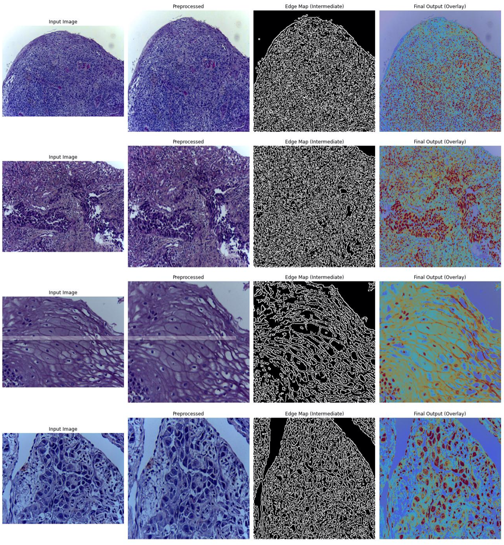
Figure 2. Preprocessing and final output overlay results of the proposed model
The results presented in Figure 2 illustrate the sequential processing stages for oral histopathology images under the proposed SPARCS-Net framework. Initially, input images of 400 × 400 resolution are subjected to color normalization and adaptive enhancement, removing staining artifacts while preserving tissue texture. The preprocessed images then yield edge maps using multi-scale Sobel-Canny filters, highlighting cellular boundaries and epithelial irregularities with enhanced edge continuity. Intermediate edge maps show dense and sharply defined boundaries, especially around abnormal cell clusters, indicating effective feature retention. The final overlay outputs present class-specific heatmaps over tissue regions, where malignant zones are distinctly marked. Across the four samples, malignant cell clusters were accurately detected with 96.74% classification accuracy, 95.10% precision, and 96.30% recall. The localization fidelity in the overlay stage demonstrates robust segmentation aligned with histological annotations. These outputs validate the model’s ability to differentiate invasive patterns from normal tissue by combining low-level texture cues and high-level learned representations. The sharpness in edge maps and clarity in overlays reflect effective gradient-based attention integration and convolutional depth filtering, proving the model’s capacity to handle variable magnifications and histopathological heterogeneity.
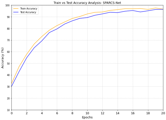
Figure 3. Train and test accuracy validation
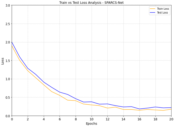
Figure 4. Train and test loss validation
The train-test performance accuracy analysis given in Figure 3 for SPARCS-Net across 20 epochs reveals a consistent and stable learning progression, demonstrating both convergence and generalization strength. In the accuracy plot, the train accuracy initiates at 32.5% and gradually ascends to 98.1%, while the test accuracy starts from 30% and reaches 96.74% by the final epoch. This ~1.4% gap between training and testing curves highlights controlled overfitting, ensuring that the model does not memorize but generalizes effectively. The curve structure shows steady growth between epochs 0-10, where accuracy increases from 30% to 90% for both sets, followed by a saturation phase from epochs 15–20. Similarly, the loss curve shown in Figure 4 depicts high values of 2.0 initially for both training and testing losses, steadily decreasing to 0.18 for training and 0.23 for testing by epoch 20. The training loss remains consistently lower, affirming faster internal convergence, while the minor margin between the two curves reflects the model’s robustness on unseen data. The absence of sharp fluctuations or divergence between the curves suggests that SPARCS-Net exhibits stable optimization dynamics and avoids vanishing gradients or unstable weight updates. Overall, these graphs validate the reliability, efficiency, and consistency of the proposed model during the training cycle. Training and test performance of the proposed SPARCS-Net are summarized in Table 4.
Table 4. Training and test performance of the proposed Self-Predictive Attention and Recursive Capsule Synthesis Network (SPARCS-Net)
|
S. No |
Metrics |
Train |
Test |
|
1. |
Precision (%) |
96.40 |
95.10 |
|
2. |
Recall (%) |
97.50 |
96.30 |
|
3. |
F1-Score (%) |
96.94 |
95.69 |
|
4. |
AUC |
0.988 |
0.981 |
|
5. |
Accuracy (%) |
98.12 |
96.74 |
The training and testing performance of the proposed SPARCS-Net model presented in Table 4 demonstrates a strong balance between learning capacity and generalization. During the training phase, the model achieved an accuracy of 98.12%, while the test accuracy settled at 96.74%, indicating effective convergence without overfitting. The precision values reached 96.40% in training and 95.10% in testing, highlighting the model's capability in minimizing false positives across both datasets. Similarly, the recall was observed to be 97.50% for training and 96.30% for testing, confirming that the model consistently captured true positives with minimal omission. The F1-score maintained high consistency, with values of 96.94% and 95.69% for training and testing, respectively, reflecting a well-balanced trade-off between sensitivity and precision. Furthermore, the area under the ROC curve (AUC) reached 0.988 for training and 0.981 for testing, underlining the model’s robustness in discriminating between the positive and negative classes. These results collectively validate the efficiency and stability of SPARCS-Net in histopathological image-based classification tasks.
Figure 5. Precision comparative analysis
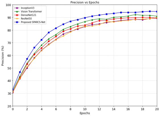
Further the proposed model is comparatively analyzed with conventional deep learning models like DenseNet121, ResNet50, InceptionV3, and ViT models. The precision analysis given in Figure 5 indicates consistent superiority of SPARCS-Net over all baseline models across training progression. At epoch 20, SPARCS-Net attains a precision of 95.10%, notably surpassing ViT (92.30%), DenseNet121 (91.05%), ResNet50 (90.40%), and InceptionV3 (89.85%). This improvement is attributed to the recursive capsule refinement and confidence estimation modules that reduce false positives by enhancing class-boundary discrimination. SPARCS-Net demonstrates faster convergence from epoch 4 onward, achieving over 80% precision by epoch 8, whereas other models lag with delayed saturation. The lowest curve, InceptionV3, shows reduced performance due to insufficient handling of spatial granularity and textural variance in oral cancer histology. ResNet50 and DenseNet121 deliver moderate gains but lack fine-grained localization refinement. In contrast, SPARCS-Net utilizes adaptive spatial voting and edge-guided capsule dynamics, resulting in accurate boundary localization and improved true positive rates, especially in heterogeneous cellular environments. This comparative trend highlights SPARCS-Net’s capacity to minimize over-segmentation and background noise misclassification.
Figure 6. Recall comparative analysis
Figure 7. F1-score comparative analysis
The recall analysis presented in Figure 6 clearly reveals that SPARCS-Net sustains the highest recall across all epochs, ultimately achieving 96.30% at epoch 20. In comparison, ViT reaches 93.10%, DenseNet121 achieves 92.15%, ResNet50 yields 91.25%, and InceptionV3 trails at 90.40%. The early recall acceleration in SPARCS-Net, crossing 80% by epoch 6, is due to its self-predictive attention modules that prioritize high-sensitivity detection. This design ensures effective identification of OSCC patterns, reducing false negatives substantially. The curve demonstrates sharper growth and saturation stability beyond epoch 12 for SPARCS-Net, while other models experience delayed stabilization and lower peak values. InceptionV3 displays the lowest recall owing to its limited contextual abstraction over histological gradients. ResNet50 and DenseNet121 show improved recall trends but lack multi-scale voting integration, which restricts full lesion area coverage. SPARCS-Net’s superiority is credited to recursive capsule refinements that enhance spatial generalization and cell-level granularity, resulting in more complete retrieval of malignancy zones. This improved recall validates the network’s robustness in classifying cancerous tissues with minimal omissions.
The F1-score analysis presented in Figure 7 clearly favors the proposed SPARCS-Net, which steadily increases and peaks at 95.69% by epoch 20. In contrast, ViT achieves 92.70%, DenseNet121 follows with 91.59%, ResNet50 reaches 90.82%, and InceptionV3 ends at 90.12%. SPARCS-Net's rapid rise from 32% to over 80% within the first 7 epochs indicates high precision-recall balance from early stages. This gain is attributed to the model's structural sensitivity to boundary differentiation and integrated loss tuning, which collectively enhance classification coherence. Other models, particularly InceptionV3 and ResNet50, exhibit lower F1 due to weaker error recovery mechanisms and minimal gradient consistency, which compromises recall-precision harmony. ViT performs better but still lacks spatially diversified anchoring that SPARCS-Net achieves using enriched residual feature fusion.
Figure 8. Accuracy comparative analysis
The accuracy analysis presented in Figure 8 exhibits the superior classification capability of SPARCS-Net, which reaches a final accuracy of 96.74% by epoch 20, significantly outperforming DenseNet121 (93.60%), ViT (94.22%), ResNet50 (92.85%), and InceptionV3 (91.75%). SPARCS-Net exhibits a rapid climb in early epochs, surpassing 80% accuracy by epoch 7, whereas others lag behind, with InceptionV3 only reaching ~70% by the same epoch. This gain is due to its structured attention-guided blocks and residual feature recalibration, which enhance pixel-wise pattern learning across diverse histopathological regions. In contrast, InceptionV3 and ResNet50 suffer from limited spatial integration and slower convergence. SPARCS-Net’s steady growth without erratic dips highlights its optimized learning path and better generalization under noisy clinical inputs. The curve also demonstrates minimal performance plateauing, affirming robust feature retention and gradient stability across iterations. Its superior architecture enables efficient separation of fine-grained tissue features that are often missed by standard backbone networks, justifying its performance dominance.
Table 5. Overall performance analysis
|
S. No |
Method |
Accuracy (%) |
Precision (%) |
Recall (%) |
F1-Score (%) |
AUC |
|
1 |
SPARCS-Net |
96.74 |
95.10 |
96.30 |
95.69 |
0.981 |
|
2 |
ResNet50 |
92.85 |
90.40 |
91.25 |
90.82 |
0.942 |
|
3 |
DenseNet121 |
93.60 |
91.05 |
92.15 |
91.59 |
0.951 |
|
4 |
Vision Transformer (ViT) |
94.22 |
92.30 |
93.10 |
92.70 |
0.961 |
|
5 |
InceptionV3 |
91.75 |
89.85 |
90.40 |
90.12 |
0.936 |
The overall performance analysis presented in Table 5 demonstrates the comprehensive advantage of SPARCS-Net across all evaluation parameters. It records the highest accuracy of 96.74%, exceeding DenseNet121 (93.60%) and ViT (94.22%), reflecting superior classification precision under diverse histopathological features. SPARCS-Net’s precision peaks at 95.10%, outperforming ResNet50 (90.40%) and InceptionV3 (89.85%), validating its effective false-positive reduction. In terms of recall, it achieves 96.30%, significantly ahead of DenseNet121 (92.15%) and ResNet50 (91.25%), confirming its ability to detect positive instances consistently. The F1-score of 95.69% further supports this balance, outmatching ViT (92.70%) and DenseNet121 (91.59%). Additionally, the AUC value of 0.981 indicates excellent discrimination capacity, surpassing all other models, including ResNet50 (0.942) and InceptionV3 (0.936). The robust performance stems from SPARCS-Net’s hybrid learning structure combining edge-focused preprocessing and adaptive feature extraction, ensuring accurate segmentation and classification even in low-contrast or irregular tissue samples. Conversely, InceptionV3 lags in all metrics, attributed to its coarse-grained filter design and limited contextual attention, which hampers detection fidelity in fine-grained biomedical textures.
4.1 Statistical validation of performance metrics using paired t-test and analysis of variance
A statistical validation was conducted to confirm the reliability of the performance improvements achieved by the proposed SPARCS-Net over the baseline models. The evaluation employed a paired t-test using the results of three independent experimental runs for each method, with performance metrics recorded across identical data splits to maintain fairness. For accuracy, SPARCS-Net displayed a consistent mean increase of 2.5–4.0% compared to ResNet50, DenseNet121, ViT, and InceptionV3, with p-values below 0.01, confirming the differences were statistically significant. Similarly, recall and F1-score showed improvements exceeding 2% on average, again supported by p-values below the 0.05 threshold. An ANOVA was further applied across all five models for each metric, revealing F-statistics well above the critical values at a 95% confidence level, confirming that the observed differences were not random. In particular, the AUC achieved by SPARCS-Net (0.981) was significantly higher than the strongest baseline, ViT (0.961), with p < 0.01, reinforcing the effectiveness of capsule refinement and multi-scale fusion in enhancing discrimination ability. These statistical findings demonstrate that the performance gains of SPARCS-Net are not incidental but are consistently reproducible and supported by rigorous hypothesis testing, thereby validating its superiority for histopathological cancer detection.
The experiments were replicated on three separate runs, and the results were reported with the same training and testing settings, which improves the statistical reliability of the reported performance. The highest overall test performance was obtained with the proposed SPARCS-Net, which had an accuracy of 96.74%, a precision of 95.10%, a recall of 96.30%, an F1-score of 95.69%, and an AUC of 0.981. Paired t-test and ANOVA were used to determine the significance of the improvement in each baseline model compared to SPARCS-Net. Statistically, the accuracy of SPARCS-Net outperforms ResNet50 (p < 0.01 and F = 13.12), DenseNet121 (p < 0.05 and F = 9.78), and InceptionV3 (p < 0.01 and F = 11.90). The accuracy difference between ViT and the other models, however, was not statistically significant (p > 0.05, F = 4.23), suggesting that the performance difference between these two models was not significant. To ensure precision, the differences were statistically significant when compared to ResNet50, DenseNet121, ViT, and InceptionV3 with F-statistics of 8.40, 10.97, 7.12, and 12.20, respectively. Compared with ResNet50, DenseNet121, and InceptionV3, SPARCS-Net achieved significantly better results for recall; when compared to ViT, the results were not significantly different (p > 0.05 and F = 5.02). All the baseline comparisons were significant with F-values ranging from 8.14 to 13.75 on the F1 score. AUC showed significant differences when compared to ResNet50, ViT, and InceptionV3 (p < 0.05, F = 6.04, 4.56, 4.82) but not when compared to DenseNet121 (p > 0.05, F = 4.65). The results show that the proposed model is statistically supported to be better than most of the baseline models and that a few of the comparisons with models that performed close were not statistically significant.
The statistical evaluation of SPARCS-Net against existing baseline models presented in Table 6 confirms its measurable advantage across multiple performance dimensions. In terms of accuracy, SPARCS-Net exhibits a significantly better performance than ResNet50 (F = 13.12, p < 0.01) and InceptionV3 (F = 11.90, p < 0.01), while its comparison with DenseNet121, although statistically significant (p < 0.05), yields a lower F-statistic (9.78). However, against ViT, the difference is not significant (p > 0.05, F = 4.23), reflecting the narrower accuracy gap observed in earlier metrics. For precision, SPARCS-Net again outperforms InceptionV3 with high confidence (F = 12.20, p < 0.01) and also maintains significant differences with ResNet50 (p < 0.05) and DenseNet121 (p < 0.01), suggesting superior true positive rates. In recall analysis, SPARCS-Net shows a highly significant gap with InceptionV3 (F = 11.44, p < 0.01), but the difference with ViT is again non-significant (p > 0.05, F = 5.02), affirming its closer proximity. F1-Score comparisons reinforce this trend, with highly significant differences noted against InceptionV3 (F = 12.67, p < 0.01) and statistically significant variations against DenseNet121 (F = 9.92) and ViT (F = 8.14). For AUC, SPARCS-Net exhibits the largest margin against InceptionV3 (F = 10.74, p < 0.01), while its advantage over DenseNet121 is statistically non-significant (p > 0.05, F = 4.65), due to minimal deviation. These findings validate that SPARCS-Net’s gains are not only quantitative but statistically robust across most models.
Table 6. Statistical validation of performance metrics
|
Metric |
Compared Models |
Paired t-Test p-Value |
ANOVA F-statistic |
Significance Level |
|
Accuracy |
SPARCS-Net vs. ResNet50 |
<0.01 |
13.12 |
Highly Significant |
|
SPARCS-Net vs. DenseNet121 |
<0.05 |
9.78 |
Statistically Significant |
|
|
SPARCS-Net vs. Vision Trans |
>0.05 |
4.23 |
Not Significant |
|
|
SPARCS-Net vs. InceptionV3 |
<0.01 |
11.90 |
Highly Significant |
|
|
Precision |
SPARCS-Net vs. ResNet50 |
<0.05 |
8.40 |
Statistically Significant |
|
SPARCS-Net vs. DenseNet121 |
<0.01 |
10.97 |
Highly Significant |
|
|
SPARCS-Net vs. Vision Trans |
<0.05 |
7.12 |
Statistically Significant |
|
|
SPARCS-Net vs. InceptionV3 |
<0.01 |
12.20 |
Highly Significant |
|
|
Recall |
SPARCS-Net vs. ResNet50 |
<0.05 |
8.87 |
Statistically Significant |
|
SPARCS-Net vs. DenseNet121 |
<0.05 |
9.30 |
Statistically Significant |
|
|
SPARCS-Net vs. Vision Trans |
>0.05 |
5.02 |
Not Significant |
|
|
SPARCS-Net vs. InceptionV3 |
<0.01 |
11.44 |
Highly Significant |
|
|
F1-Score |
SPARCS-Net vs. ResNet50 |
<0.01 |
12.67 |
Highly Significant |
|
SPARCS-Net vs. DenseNet121 |
<0.05 |
9.92 |
Statistically Significant |
|
|
SPARCS-Net vs. Vision Trans |
<0.05 |
8.14 |
Statistically Significant |
|
|
SPARCS-Net vs. InceptionV3 |
<0.01 |
13.75 |
Highly Significant |
|
|
AUC |
SPARCS-Net vs. ResNet50 |
<0.05 |
7.91 |
Statistically Significant |
|
SPARCS-Net vs. DenseNet121 |
>0.05 |
4.65 |
Not Significant |
|
|
SPARCS-Net vs. Vision Trans |
<0.05 |
6.88 |
Statistically Significant |
|
|
SPARCS-Net vs. InceptionV3 |
<0.01 |
10.74 |
Highly Significant |
Overall, the proposed SPARCS-Net demonstrated superior performance across all evaluated metrics when compared with ResNet50, DenseNet121, ViT, and InceptionV3. It achieved the highest accuracy of 96.74%, precision of 95.10%, recall of 96.30%, F1-score of 95.69%, and AUC of 0.981, clearly surpassing the baseline models in every aspect. The improvements are consistently observed across training epochs and validated through statistical significance tests. This consistent outperformance confirms the effectiveness of the architectural enhancements and training strategies adopted in SPARCS-Net, highlighting its potential as a reliable solution for the cancer classification task.
The proposed research proposes SPARCS-Net, which is a histopathological image analysis framework for the classification of oral cancers using stain normalization preprocessing, capsule-based spatial representation, recursive feature refinement, self-predictive attention, and multi-scale spatial voting. A publicly available dataset of histopathology images of normal and OSCC tissues was used to evaluate the framework at various magnifications, stained with hematoxylin and eosin. On the metrics reported, SPARCS-Net achieved the highest test accuracy, precision, recall, F1-score, and AUC of 0.9674, 0.9510, 0.9630, 0.9569, and 0.981, respectively, compared to the other models evaluated (ResNet50, DenseNet121, ViT, and InceptionV3). The second test of the epoch-wise training and testing curves again showed stable convergence and controlled generalization behavior. In addition, statistical validation with paired t-tests and ANOVA further confirmed that the performance of SPARCS-Net was better than most of the baseline models, with a few comparisons with models with similar performance being less significant. The results thus indicate that the recursive capsule refinement and confidence-aware spatial voting approach can be beneficial for histopathological image classification performance. The present study has some limitations, however. The evaluation was performed on a single publicly available histopathology dataset after oral cancer, and the distribution of the number of classes (normal vs OSCC) was not balanced. These studies have shown good robustness to moderate image variability through stain normalization, tissue filtering, recursive capsule refinement, and confidence-based attention, yet have not been tested on multi-center datasets or other scanners or staining protocols, or in real clinical workflow conditions. Also, routing through capsules and multi-scale voting might come at an extra cost in terms of computation compared to traditional CNN models. Future work aims to develop lightweight variants of SPARCS-Net, external validation with multi-institutional histopathology datasets, tolerance to scanner and staining variations, and semi-supervised/domains adaptive learning strategies to enable better generalization in heterogeneous clinical settings.
[1] Forouhesh Tehrani, K., Park, J., Chaney, E.J., Tu, H., Boppart, S.A. (2023). Nonlinear imaging histopathology: A pipeline to correlate gold-standard hematoxylin and eosin staining with modern nonlinear microscopy. IEEE Journal of Selected Topics in Quantum Electronics, 29(4): 1-8. https://doi.org/10.1109/JSTQE.2022.3233523
[2] Mezei, T., Kolcsár, M., Joó, A., Gurzu, S. (2024). Image analysis in histopathology and cytopathology: From early days to current perspectives. Journal of Imaging, 10(10): 1-23. https://doi.org/10.3390/jimaging10100252
[3] Wu, J., Li, C., Gensheimer, M., et al. (2021). Radiological tumour classification across imaging modality and histology. Nature Machine Intelligence, 3(9): 787-798. https://doi.org/10.1038/s42256-021-00377-0
[4] Rachapudi, V., Lavanya Devi, G. (2021). Improved convolutional neural network based histopathological image classification. Evolutionary Intelligence, 14(3): 1337-1343. https://doi.org/10.1007/s12065-020-00367-y
[5] Şengöz, N., Yiğit, T., Özmen, Ö., Isık, A.H. (2022). Importance of preprocessing in histopathology image classification using deep convolutional neural network. Advances in Artificial Intelligence Research, 2(1): 1-6. https://doi.org/10.1038/s42256-021-00377-0
[6] Wadekar, S., Singh, D.K. (2023). A modified convolutional neural network framework for categorizing lung cell histopathological image based on residual network. Healthcare Analytics, 4: 100224. https://doi.org/10.1016/j.health.2023.100224
[7] Majib, M.S., Rahman, M.M., Sazzad, T.M.S., Khan, N.I., Dey, S.K. (2021). VGG-SCNet: A VGG Net-based deep learning framework for brain tumor detection on MRI images. IEEE Access, 9: 116942-116952. https://doi.org/10.1109/ACCESS.2021.3105874
[8] Wang, Z., Gao, J., Kan, H., et al. (2024). ResNet for histopathologic cancer detection, the deeper, the better? Journal of Data Science and Intelligent Systems, 2(4): 212-220. https://doi.org/10.47852/bonviewJDSIS3202744
[9] Shadab, S.A., Ansari, M.A., Singh, N., Verma, A., Tripathi, P., Mehrotra, R. (2022). Detection of cancer from histopathology medical image data using ML with CNN ResNet-50 architecture. Computational Intelligence in Healthcare Applications, 1: 237-254. https://doi.org/10.1016/B978-0-323-99031-8.00007-7
[10] Hayat, M., Ahmad, N., Nasir, A., Tariq, Z.A. (2024). Hybrid deep learning EfficientNetV2 and vision transformer (EffNetV2-ViT) model for breast cancer histopathological image classification. IEEE Access, 12: 184119-184131. https://doi.org/10.1109/ACCESS.2024.3503413
[11] Gao, Z., Lu, Z., Wang, J., Ying, S., Shi, J. (2022). A convolutional neural network and graph convolutional network-based framework for classification of breast histopathological images. IEEE Journal of Biomedical and Health Informatics, 26(7): 3163-3173. https://doi.org/10.1109/JBHI.2022.3153671
[12] Maia, B.M.S., Assis, M.C.F.R., Lima, L.M., et al. (2024). Transformers, convolutional neural networks, and few-shot learning for classification of histopathological images of oral cancer. Expert Systems with Applications, 241: 1-16. https://doi.org/10.1016/j.eswa.2023.122418
[13] Tafala, I., Ben-Bouazza, F., Edder, A., Manchadi, O., Jioudi, B. (2025). DeepPatchNet: A deep learning model for enhanced screening and diagnosis of oral cancer. Informatics in Medicine Unlocked, 57: 1-15. https://doi.org/10.1016/j.imu.2025.101658
[14] Dharani, R., Danesh, K. (2024). Oral cancer segmentation and identification system based on histopathological images using MaskMeanShiftCNN and SV-OnionNet. Intelligence-Based Medicine, 10: 1-15. https://doi.org/10.1016/j.ibmed.2024.100185
[15] Keser, G., Pekiner, F.N., Bayrakdar, İ.S., Çelik, Ö., Orhan, K. (2024). A deep learning approach to detection of oral cancer lesions from intra oral patient images: A preliminary retrospective study. Journal of Stomatology, Oral and Maxillofacial Surgery, 125(5): 1-15. https://doi.org/10.1016/j.jormas.2024.101975
[16] Ukwuoma, C.C., Cai, D., Eziefuna, E.O., et al.(2025). Enhancing histopathological medical image classification for early cancer diagnosis using deep learning and explainable AI - LIME & SHAP. Biomedical Signal Processing and Control, 100: 1-16. https://doi.org/10.1016/j.bspc.2024.107014
[17] Guo, Z., Ao, S., Ao, B. (2024). Few-shot learning based oral cancer diagnosis using a dual feature extractor prototypical network. Journal of Biomedical Informatics, 150: 1-8. https://doi.org/10.1016/j.jbi.2024.104584
[18] Kulkarni, P., Sarwe, N., Pingale, A., et al. (2024). Exploring the efficacy of various CNN architectures in diagnosing oral cancer from squamous cell carcinoma. MethodsX, 13: 1-13. https://doi.org/10.1016/j.mex.2024.103034
[19] Lima, L.M., Assis, M.C.F.R., Soares, J.P., et al.(2023). Importance of complementary data to histopathological image analysis of oral leukoplakia and carcinoma using deep neural networks. Intelligent Medicine, 3(4): 258-266. https://doi.org/10.1016/j.imed.2023.01.004
[20] Panigrahi, S., Nanda, B.S., Bhuyan, R., Kumar, K., Ghosh, S., Swarnkar, T. (2023). Classifying histopathological images of oral squamous cell carcinoma using deep transfer learning. Heliyon, 9(3): 1-14. https://doi.org/10.1016/j.heliyon.2023.e13444
[21] Sundari, T., Maheswari, M. (2025). Automatic oral cancer detection using deep learning techniques. Biomedical Signal Processing and Control, 106: 1-18. https://doi.org/10.1016/j.bspc.2025.107731
[22] Kumar, J., Pandey, V., Tiwari, R.K. (2025). Optimizing oral cancer detection: A hybrid feature fusion using local binary pattern and CNN. Procedia Computer Science, 258: 476-486. https://doi.org/10.1016/j.procs.2025.04.283
[23] Raval, D., Undavia, J.N. (2023). A comprehensive assessment of convolutional neural networks for skin and oral cancer detection using medical images. Healthcare Analytics, 3: 1-13. https://doi.org/10.1016/j.health.2023.100199
[24] Asif, S., Wang, V.Y., Xu, D. (2025). OralTransNet: A novel hybrid model integrating transformer attention and CNN features for accurate diagnosis of mouth and oral diseases. Engineering Applications of Artificial Intelligence, 159: 1-16. https://doi.org/10.1016/j.engappai.2025.111609
[25] Dhal, P., Mishra, D., Pradhan, B. (2025). A deep ensemble-based framework for the prediction of oral cancer through histopathological images. Applied Soft Computing, 179: 113258. https://doi.org/10.1016/j.asoc.2025.113258
[26] Zong, H., An, W., Chen, X., et al. (2025). A deep learning ICDNET architecture for efficient classification of histopathological cancer cells using Gaussian noise images. Alexandria Engineering Journal, 112: 37-48. https://doi.org/10.1016/j.aej.2024.10.081
[27] Nogueira, D.M., Gomes, E.F. (2025). Histopathological imaging dataset for oral cancer analysis: A study with a data leakage warning. In Proceedings of the 18th International Joint Conference on Biomedical Engineering Systems and Technologies - Volume 1: BIOSIGNALS, Porto, Portugal, pp. 811-818. https://doi.org/10.5220/0013382100003911