Sutikno*![]() | Helmie A. Wibawa
| Helmie A. Wibawa![]() | Indra Waspada
| Indra Waspada![]()
© 2026 The authors. This article is published by IIETA and is licensed under the CC BY 4.0 license (http://creativecommons.org/licenses/by/4.0/).
OPEN ACCESS
Rice leaf diseases significantly reduce crop yield and threaten global food security. Early and accurate detection of disease symptoms is therefore essential for improving agricultural productivity. Computer vision and machine learning techniques have recently shown promising potential for plant disease identification using leaf images. However, accurately distinguishing visually similar diseases remains challenging due to subtle variations in texture and color patterns. This study proposes a multi-descriptor feature fusion approach for rice leaf disease classification. Three complementary handcrafted descriptors—Gray Level Co-occurrence Matrix (GLCM), Local Binary Pattern (LBP), and Color Histogram (CH)—are combined to capture diverse visual characteristics of diseased rice leaves. GLCM extracts macrotexture information such as large spots and tissue damage, LBP captures microtexture variations including fine lesions and surface irregularities, and CH represents the global color distribution associated with disease symptoms. The combined feature representation is then classified using a Random Forest classifier. Experiments were conducted on two publicly available datasets: Rice Leaf Disease dataset 1 (RLD1) and Rice Leaf Disease dataset 2 (RLD2). The proposed descriptor fusion approach achieved classification accuracies of 97.22% on RLD1 and 99.41% on RLD2, outperforming individual descriptors and other descriptor combinations. These results demonstrate that integrating complementary texture and color features significantly improves the discriminative capability of machine learning models for rice leaf disease classification. The proposed approach provides an effective and computationally efficient solution for automated crop disease monitoring in smart agriculture systems.
rice leaf disease classification, feature fusion, gray level co-occurrence matrix, local binary pattern, color histogram, machine learning, smart agriculture
As one of the world's top rice producers, Indonesia relies heavily on rice to sustain national food security. In 2025, the country is forecasted to rank fourth globally in rice production [1]. The rice farming sector provides livelihoods for millions of farmers and plays a strategic role in maintaining the community's economic and social stability. Nonetheless, rice productivity is often hindered by leaf diseases, including bacterial leaf blight, brown spot, leaf scald, and narrow brown spot. These diseases can reduce crop yields by up to 50% if not detected and treated early [2]. Early detection of rice leaf diseases is crucial for reducing crop losses and enhancing agricultural management efficiency.
Artificial intelligence-based technologies have demonstrated significant potential for detecting plant diseases through image analysis. Image-based methods enable faster, more accurate, and more efficient identification of rice leaf disease symptoms than traditional techniques. Research on computer vision for rice leaf disease detection and classification started about ten years ago. The main factors affecting the accuracy of results are feature extraction and classification. Generally, there are two feature extraction methods: non-handcrafted and handcrafted. The non-handcrafted approach automatically extracts features from rice leaf images using deep learning models. Examples of these models include Convolutional Neural Network (CNN) [3], VGG-16 [4, 5], InceptionResNetV2 [6], GoogleNet [7, 8], Alexnet [9, 10], and YOLO [11]. Meanwhile, Darmawan et al. [12] used Deep Metric Learning.
Handcrafted features extract characteristics from leaf visual traits, including color, texture, and shape. Pothen and Pai [13] compared the extraction of Local Binary Patterns (LBP) and Histograms of Oriented Gradients (HOG). The results showed that HOG was superior to LBP. Sulistyaningrum et al. [14] combined color extraction, Gray Level Co-occurrence Matrix (GLCM), and shape features such as centroid, eccentricity, and axis length. Rumy et al. [15] combined Color Histogram (CH), Hu Moments, GLCM, and Haralick texture using Random Forest (RF) as a classifier. Zhao et al. [16] combined GLCM and Pearson Correlation Analysis (PCA). Combining several appropriate features has been shown to improve accuracy [17]. Coarse pattern structures, such as spots, wrinkles, and color changes, are characteristic of rice leaf diseases. Therefore, this study combined three suitable descriptors: GLCM, LBP, and CH. GLCM measures second-order statistical texture information, capturing coarse patterns such as spots and leaf tissue damage. LBP extracts local texture variations, enabling the identification of subtle surface changes such as fine wrinkles and small lesions. CH evaluates global color distribution, which is essential for detecting discoloration and chlorosis commonly associated with rice leaf diseases. The combination of LBP, GLCM, and CH provides a rich feature representation by capturing micro-texture, macro-texture, and color changes, enabling superior, accurate, and stable classification of various leaf diseases [18]. These three descriptors were selected because they provide non-redundant and mutually reinforcing feature characteristics. The combination of these feature extraction methods is expected to improve the accuracy of rice leaf disease classification.
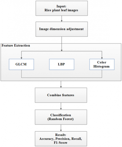
The proposed system's stages are shown in Figure 1. In general, the system consists of four main steps: image dimension adjustment, feature extraction, combining features, and classification. The image dimension adjustment is performed during preprocessing to ensure all images have uniform dimensions, enabling each extraction algorithm to operate consistently. In the feature extraction stage, three complementary descriptors, GLCM, LBP, and CH, are applied in parallel. GLCM extracts macrotexture patterns, such as large spots or leaf tissue damage. LBP captures microtextures, such as fine dots and surface irregularities. CH maps color variations arising from physiological changes in diseased leaves. Each descriptor generates a feature vector that is then combined in the feature combination stage to form a more comprehensive image representation. This combined representation strengthens the model's ability to distinguish subtle differences between disease classes. In the final stage, the combined features are fed into an RF classifier to determine the disease category for each image sample. Performance evaluation is conducted using accuracy, precision, recall, and F1-score metrics to assess the system's overall effectiveness.
Figure 1. The stages of the proposed system for rice leaf classification
2.1 Image dimension adjustment
Image dimension adjustment changes an image's size. This study utilizes two image datasets. The image in the first dataset measures 1,440 × 1,920 pixels, while the image in the second dataset measures 1,600 × 1,600 pixels. Both datasets are resized to 128 × 128 pixels. During preprocessing, we use the original images and resize them only to preserve the characteristics of the rice leaves.
2.2 Feature extraction process
The descriptors used in this feature extraction include GLCM, LBP, and CL. GLCM detects coarse patterns, such as spots or leaf tissue damage, effectively highlighting them. LBP analyzes leaf surfaces, such as wrinkles and spots. CL assesses color changes associated with rice leaf diseases.
2.2.1 Gray Level Co-occurrence Matrix
GLCM is a widely recognized technique for extracting texture features, developed by Haralick et al. [19]. GLCM calculates the frequency of pairs of pixels with specific gray levels that occur together at a given direction and distance within an image. This descriptor generates a G × G matrix, where each element represents the frequency with which pairs (i, j) appear together. Suppose P(i,j) is the probability of pixels with intensities i and j appearing together, and G is the number of gray levels. In that case, it is possible to derive statistical features [20]. Contrast measures the difference between pixels and is expressed as in Eq. (1). homogeneity assesses how closely the element distribution aligns with the GLCM diagonal and is expressed using Eq. (2). energy is evaluated based on the compactness or uniformity of the matrix and is calculated as shown in Eq. (3). correlation, on the other hand, measures the similarity of patterns between neighboring pixels, as defined by Eq. (4). In these formulas, $\mu_{\mathrm{i}}$ and $\mu_{\mathrm{j}}$ represent the mean values of row index i and column index j in the GLCM, respectively, and $\sigma_i$ and $\sigma_j$ are the standard deviations of the distributions of values i and j.
$Contrast=\sum_{i=1}^G \sum_{j=1}^G(i-j)^2 \cdot P(i, j)$ (1)
$Homogeneity=\sum_{i=1}^G \sum_{j=1}^G \frac{P(i, j)}{1+|i-j|}$ (2)
$Energy=\sum_{i=1}^G \sum_{j=1}^G[P(i, j)]^2$ (3)
$Correlation=-\sum_{i=1}^G \sum_{j=1}^G \frac{\left(i-\mu_i\right)\left(j-\mu_i\right) \cdot P(i, j)}{\sigma_i \cdot \sigma_j}$ (4)
2.2.2 Local Binary Pattern
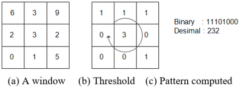
The LBP technique describes image textures by analyzing the neighborhoods of each pixel. In its simplest form, the LBP operator compares each of the eight surrounding pixels to the center pixel and assigns a binary value (0 or 1) based on whether the intensity of the neighbor is greater than or equal to that of the center pixel. These binary values are combined into a single LBP code that captures local texture information. An illustration of the LBP computation process is shown in Figure 2. The LBP feature extraction was performed using the standard configuration with eight sampling points evenly spaced around a circular neighborhood of radius 1 pixel. The rotation parameter was set to upright, preserving the spatial relationship between pixels without rotation invariance. This configuration was chosen due to its balance between computational efficiency and the ability to capture meaningful texture patterns.
Figure 2. Example of LBP calculation
Note: LBP = Local Binary Pattern.
2.2.3 Color Histogram
CH is a statistical method frequently used to illustrate the distribution of colors in digital images. This method works by calculating the frequency of each color value or combination within the image, then organizing these frequencies into a histogram [21]. The color histogram is considered a global feature because it ignores spatial information about pixels. Instead, it focuses on the relative count of pixels for each color.
Generally, when an image is represented in a specific color space, such as RGB or HSV, a histogram is generated for each color channel. For example, in the RGB color space, a color histogram can be calculated by dividing each channel (Red, Green, and Blue) into several bins (color intervals) and then counting the number of pixels in each bin. Suppose a digital image has color channels C $\in${R, G, B}, and each channel is divided into n bins; then, the histogram value Hc(k) for channel c and the kth bin can be defined as in Eq. (5). Ic(x,y) is the pixel intensity at coordinate (x,y) for channel c, Bk is the range of color values in the kth bin, d(a, Bk)=1 if a $\in$ Bk, and zero otherwise, and W×H is the image resolution.
$H_c(k)=\sum_{x=1}^W \sum_{y=1}^H \delta\left(I_c(x, y), B_k\right)$ (5)
2.3 Combine features
The result of GLCM feature extraction (fglcm) can be expressed as in Eq. (6), where fgi is the ith GLCM feature and m is the total number of features. The LDB feature extraction (fldb) output is given by Eq. (7), where fli is the ith LDB feature and n is the total number of LDB features. Meanwhile, the CH feature (fch) is given by Eq. (8), where fci is the ith CH feature and p is the total number of features. The integration of the three features is shown to coincide in Eq. (9).
$f_{g l c m}=\left[f_{g_1} f g_2 \ldots f g_m\right]$ (6)
$f_{l d b}=\left[f l_1 f l_2 \ldots f l_n\right]$ (7)
$f_{c h}=\left[fc{_1} f c_2 \ldots f c_p\right]$ (8)
$f_{c o n}=\left[f_{g l c m} f_{l d b} f_{c h}\right]$ (9)
2.4 Classification
The descriptors used in this feature extraction include GLCM, LBP, and CL. GLCM detects coarse patterns, such as spots or leaf tissue damage, effectively highlighting them. LBP analyzes leaf surfaces, such as wrinkles and spots. CL assesses color changes associated with rice leaf diseases. Random Forest (RF) is a highly effective ensemble learning technique for classification tasks. This algorithm operates by constructing multiple decision trees simultaneously and combining their predictions via majority voting to achieve more accurate, stable outcomes [22]. The primary advantage of RF is its capacity to minimize overfitting via bagging and random feature selection at each split.
The classification process starts with creating several bootstrap samples from the original dataset. Each sample is used to train a decision tree. During tree building, at each node, the algorithm considers only a random subset of features to find the best split. This method ensures that each tree in the forest has enough variation, making the combined prediction more reliable. To evaluate the quality of the split, RF usually uses Gini Impurity or Entropy. Gini Impurity measures how often a randomly chosen element will be misclassified, using Eq. (10), where pk is the proportion of samples in class k. Meanwhile, Entropy measures the uncertainty in the data split, calculated with Eq. (11). The final prediction for a sample is made through majority voting, calculated using Eq. (12), where T trees predict $\hat{y}_1, \hat{y}_2, \ldots, \hat{y}_T$.
$G=1-\sum_{k=1}^K p_k^2$ (10)
$H=-\sum_{k=1}^K p_k \log \left(p_k\right)$ (11)
$\hat{y}={mode}\left\{\hat{y}_1, \hat{y}_2, \ldots, \hat{y}_T\right\}$ (12)
2.5 Performance evaluation
The evaluation of the proposed method was conducted using accuracy, precision, recall, and F1-score, as defined in Eqs. (13)-(16), respectively [23]. Since the classification task involves multiple classes, the metrics were computed using the one-vs-all (OvA) strategy, in which each class is compared against all others. The results were then aggregated using macro averaging, assigning equal weight to each class.
Classification evaluation metrics are derived from the confusion matrix. In multiclass classification, TPi (True Positive) is the number of data points correctly identified as class i. TNi (True Negative) is the number of data points correctly identified as not belonging to class i. FPi (False Positive) indicates data points incorrectly labeled as class i, when they belong to another class. Lastly, FNi (False Negative) represents data points that should be classified as class i but are incorrectly assigned to another class.
$ Accuration =\frac{\sum_{i=1}^K T P_i+T N_i}{\sum_{i=1}^K T P_i+T N_i+F P_i+F N_i}$ (13)
$Precision_i=\frac{T P_i}{T P_i+F P_i}$ (14)
$Recall_i=\frac{T P_i}{T P_i+F N_i}$ (15)
$F 1- score _i=2 \times \frac{ { Precision }_i \times { Recall }_i}{ { Precision }_i+ { Recall }_i}$ (16)
3.1 Dataset
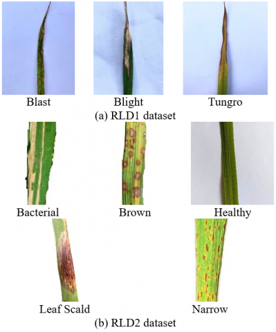
This study used two datasets: Rice Leaf Disease 1 (RLD1) and Rice Leaf Disease 2 (RLD2), as shown in Figure 3. Both datasets are publicly available on Kaggle. RLD1 is a rice leaf disease dataset collected from Southeast Sulawesi, Indonesia. It includes three classes of rice leaf diseases: blast, blight, and tungro [24], each with 80 images. Meanwhile, RLD2 contains 2,254 images divided into five classes: 438 bacterial leaf images, 464 brown leaf images, 464 healthy leaf images, 448 leaf scald images, and 440 narrow leaf images [25]. Figure 3(a) shows an example from RLD1, and Figure 3(b) shows an example from RLD2. The dataset was divided into three parts: 70% for training, 15% for validation, and 15% for testing.
Figure 3. Examples of datasets
3.2 Results and analysis
The testing was divided into two parts: single-descriptor and multi-descriptor testing. In single-descriptor testing, the four descriptors used were HOG, GLCM, LBP, and CH. The GLCM features used include contrast, correlation, energy, and homogeneity. This testing involved tuning hyperparameters for each descriptor. Multi-descriptor testing was conducted by combining all possible combinations of the four descriptors. The parameters used by the RF classifier are: 100 trees, minimum leaf size 1, and minimum sample size at the node 10.
3.2.1 Single descriptor
Single-descriptor testing aims to identify the best descriptor from four options. Testing each descriptor involves tuning the hyperparameters listed in Table 1. The results, presented in Table 2, indicate that the CH descriptor achieves the highest accuracy (Acc) and macro-average F1-score (MAF1-S) on both datasets. LBP and HOG produced nearly identical accuracy figures, with RLD1 reaching 91.67% and RLD2 reaching 98.81%. The optimal parameters for both datasets are the same: 8 bins, HSV color space, and a grid size of 1 × 1.
Table 1. Descriptor parameters set
|
Descriptor |
Parameters |
|
HOG |
Cell size: 8×8, 16×16, and 32×32 Block size: 2×2, 3×3, and 4×4 Number bins: 6, 9, and 12 |
|
GLCM |
Gray levels: 16, 32, and 64 Distances: 1, 2, and 3 Directions: 0, pi/4, pi/2, and 3×pi/4 |
|
LBP |
Radius: 1, 2, and 3 Number Points: 8, 12, and 16 |
|
CH |
Number Bins: 8, 16, and 32 Color Spaces: RGB, HSV, and LAB Grid Sizes: 1×1, 2×2, and 4×4 |
Table 2. Parameter tuning test results on single descriptors
|
Descriptor |
RLD1 Dataset |
RLD2 Dataset |
||
|
Acc (%) |
MAF1-S (%) |
Acc (%) |
MAF1-S (%) |
|
|
HOG |
77.78 |
77.62 |
86.31 |
86.00 |
|
GLCM |
41.67 |
39.75 |
63.99 |
64.19 |
|
LBP |
77.78 |
77.23 |
88.99 |
88.86 |
|
CH |
91.67 |
91.77 |
98.81 |
98.83 |
3.2.2 Multi descriptor
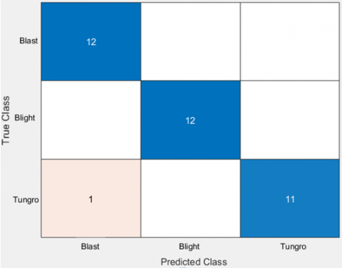
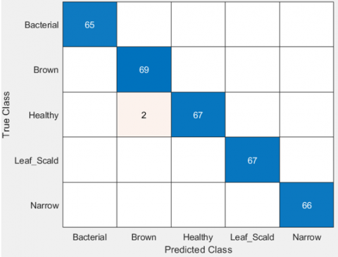
In the single descriptor test, the best parameters were identified for each descriptor. These parameters were then used in the multi-descriptor test, which also combines all possible sets of 4 descriptors (11 combinations). The results of this test were shown in Table 3. In RLD1, the highest accuracy reaches 97.22% using GLCM + CH and GLCM + LBP + CH, while in RLD2, the maximum accuracy is 99.41% with GLCM + LBP + CH. The confusion matrix for the GLCM + LBP + CH descriptor combination (proposed method) is provided in Figure 4. Figure 4(a) is the result of the confusion matrix for the RLD1 dataset, and Figure 4(b) is the result of the confusion matrix for the RLD2 dataset. Additionally, the precision and recall results for the proposed method are summarized in Table 4.
Although the GLCM descriptor has low accuracy on its own, combining it with the CH descriptor results in high accuracy. Conversely, when the CH descriptor was combined with HOG or LBP, its accuracy was reduced compared to using CH alone. LBP can also improve accuracy when combined with LBP + CH on RLD2. However, combining four descriptors (HOG, GLCM, LBP, and CH) produces lower accuracy than using CH, GLCM, GLCM + CH, or GLCM + CH + LBP. Therefore, it can be concluded that combining multiple descriptors does not always boost accuracy for rice leaf disease classification. Still, using the right combinations of descriptors can increase accuracy. For a single descriptor, CH outperforms HOG, GLCM, and LBP. The GLCM + CH pair is a more effective double descriptor than other combinations, and the GLCM + LBP + CH triple descriptor performs better than other single or triple descriptors.
Table 3. Test results on descriptor combinations
|
Dataset |
Descriptor |
Acc (%) |
MAF1-S (%) |
|
RLD1 |
HOG+GLCM |
77.78 |
77.53 |
|
HOG+LBP |
75.00 |
70.94 |
|
|
HOG+CH |
80.56 |
80.38 |
|
|
GLCM+LBP |
77.78 |
77.21 |
|
|
GLCM+CH |
97.22 |
97.22 |
|
|
LBP+CH |
88.89 |
89.07 |
|
|
HOG+GLCM+LBP |
77.78 |
76.85 |
|
|
HOG+GLCM+CH |
86.11 |
86.11 |
|
|
HOG+LBP+CH |
91.67 |
91.64 |
|
|
GLCM+LBP+CH |
97.22 |
97.22 |
|
|
HOG+GLCM+LBP+CH |
86.11 |
85.88 |
|
|
RLD2 |
HOG+GLCM |
87.80 |
87.53 |
|
HOG+LBP |
87.20 |
86.99 |
|
|
HOG+CH |
92.56 |
92.54 |
|
|
GLCM+LBP |
93.75 |
93.83 |
|
|
GLCM+CH |
99.11 |
99.11 |
|
|
LBP+CH |
98.51 |
98.53 |
|
|
HOG+GLCM+LBP |
86.90 |
86.46 |
|
|
HOG+GLCM+CH |
92.86 |
92.83 |
|
|
HOG+LBP+CH |
93.15 |
93.14 |
|
|
GLCM+LBP+CH |
99.41 |
99.42 |
|
|
HOG+GLCM+LBP+CH |
93.75 |
93.71 |
(a) RLD1 dataset
(b) RLD2 dataset
Figure 4. Confusion matrix results of the proposed method
Table 4. Precision and recall results of the proposed method
|
Dataset |
Class |
Precision (%) |
Recall (%) |
|
RLD1 |
Blast |
92.31 |
100.00 |
|
Blight |
100.00 |
100.00 |
|
|
Tungro |
100.00 |
91.67 |
|
|
RLD2 |
Bacterial |
100.00 |
100.00 |
|
Brown |
97.18 |
98.57 |
|
|
Healthy |
100.00 |
98.53 |
|
|
Leaf Scald |
100.00 |
100.00 |
|
|
Narrow |
100.00 |
100.00 |
Table 5. Comparison of the proposed method with previous studies
|
Dataset |
Methode |
Acc (%) |
MAF1-S (%) |
|
RLD1 |
HOG+SVM [13] |
69.44 |
66.82 |
|
LBP+SVM [13] |
72.22 |
71.86 |
|
|
CNN+DT [3] |
83.33 |
83.55 |
|
|
CNN+SVM [3] |
80.56 |
80.53 |
|
|
CNN+KNN [3] |
86.11 |
86.28 |
|
|
CNN+LR [3] |
58.33 |
58.65 |
|
|
Proposed |
97.22 |
97.22 |
|
|
RLD2 |
HOG+SVM [13] |
84.52 |
84.57 |
|
LBP+SVM [13] |
89.58 |
89.41 |
|
|
CNN+DT [3] |
91.96 |
91.99 |
|
|
CNN+SVM [3] |
93.45 |
93.41 |
|
|
CNN+KNN [3] |
93.45 |
93.47 |
|
|
CNN+LR [3] |
50.89 |
51.20 |
|
|
Proposed |
99.40 |
99.42 |
GLCM performs poorly when used alone because it captures only macrotexture and cannot capture color information or microdetails, which are key characteristics of rice leaf diseases. However, GLCM becomes invaluable when combined with LBP and CH because it provides a large-scale textural context that neither LBP nor CH can capture. CH, on the other hand, emerges as the most powerful descriptor on its own because most disease symptoms manifest as color changes. LBP complements both by extracting microtextural variations, such as small lesions, necrosis spots, and subtle leaf surface changes, information that cannot be obtained from either GLCM or CH. When these three descriptors are combined, particularly in the GLCM+CH and GLCM+LBP+CH combinations, classification performance improves significantly because each descriptor provides distinct, non-redundant feature dimensions, resulting in a richer, highly discriminatory representation of various rice leaf diseases.
The proposed research was then compared with previous studies, and the results were presented in Table 5. Pothen and Pai [13] proposed several stages, including segmentation using the Otsu method, feature extraction comparing HOG and LBP descriptors, and classification using an SVM with a Polynomial kernel. Pandi et al. [3] proposed using a CNN for feature extraction and compared four classifiers: Decision Tree (DT), SVM, K-Nearest Neighbors (KNN), and Logistic Regression (LR). From this table, it is clear that the proposed method outperforms previous studies.
This study presents a method for classifying rice leaf diseases. Its main contribution is combining three relevant descriptors — GLCM, LBP, and CH — in the feature extraction process for rice leaf disease classification. Test results showed that the proposed descriptor outperforms single descriptors (HOG, GLCM, LBP, and CH), double descriptors (HOG+GLCM, HOG+LBP, HOG+CH, GLCM+LBP, and LBP+CH), triple descriptors (HOG+GLCM+LBP, HOG+GLCM+CH, and HOG+LBP+CH), and the combination of all four (HOG+GLCM+LBP+CH). The proposed method achieved an accuracy of 97.22% on RLD1 and 99.41% on RLD2. Therefore, this approach appears suitable for classifying or detecting rice leaf diseases. Future research could incorporate feature selection to reduce computation time and enhance accuracy.
[1] United States Department of Agriculture. Top Producing Countries, https://www.fas.usda.gov/data/production/0422110, accessed on Oct. 1, 2025.
[2] Jiang, N., Yan, J., Liang, Y., Shi, Y., He, Z., Wu, Y., Peng, J. (2020). Resistance genes and their interactions with bacterial blight/leaf streak pathogens (Xanthomonas oryzae) in rice (Oryza sativa L.)—An updated review. Rice, 13(1): 3. https://doi.org/10.1186/s12284-019-0358-y
[3] Pandi, S.S., Kumar, K.D., Raja, K., Senthilselvi, A. (2024). Rice plant leaf disease classification using machine learning algorithm. In 2024 2nd International Conference on Advancement in Computation & Computer Technologies (InCACCT), Gharuan, India, pp. 59-63. https://doi.org/10.1109/InCACCT61598.2024.10551249
[4] Anami, B.S., Malvade, N.N., Palaiah, S. (2020). Deep learning approach for recognition and classification of yield affecting paddy crop stresses using field images. Artificial Intelligence in Agriculture, 4: 12-20. https://doi.org/https://doi.org/10.1016/j.aiia.2020.03.001
[5] Jiang, Z., Dong, Z., Jiang, W., Yang, Y. (2021). Recognition of rice leaf diseases and wheat leaf diseases based on multi-task deep transfer learning. Computers and Electronics in Agriculture, 186: 106184. https://doi.org/10.1016/j.compag.2021.106184
[6] Krishnamoorthy, N., Prasad, L.N., Kumar, C.P., Subedi, B., Abraha, H.B., Sathishkumar, V.E. (2021). Rice leaf diseases prediction using deep neural networks with transfer learning. Environmental Research, 198: 111275. https://doi.org/10.1016/j.envres.2021.111275
[7] Yakkundimath, R., Saunshi, G., Anami, B., Palaiah, S. (2022). Classification of rice diseases using convolutional neural network models. Journal of The Institution of Engineers (India): Series B, 103(4): 1047-1059. https://doi.org/10.1007/s40031-021-00704-4
[8] Yang, L., Yu, X., Zhang, S., Long, H., Zhang, H., Xu, S., Liao, Y. (2023). GoogLeNet based on residual network and attention mechanism identification of rice leaf diseases. Computers and Electronics in Agriculture, 204: 107543. https://doi.org/10.1016/j.compag.2022.107543
[9] Canlas, C.J.N., Cortez, C.M.M., Cruz, R.A.M.D., Padua, J.R.G., Timbol, A.G.G., Yumul, J.G., Materum, L. (2022). Camera radial distance-based accuracy of a bacterial blight, brown spot, and rice blast plant disease identification system for remote communications. Journal of Image and Graphics, 10(4): 158-165. https://doi.org/10.18178/joig.10.4.158-165
[10] Simhadri, C.G., Kondaveeti, H.K. (2023). Automatic recognition of rice leaf diseases using transfer learning. Agronomy, 13(4): 961. https://doi.org/10.3390/agronomy13040961
[11] Deng, J., Yang, C., Huang, K., Lei, L., Ye, J., Zeng, W., Zhang, Y. (2023). Deep-learning-based rice disease and insect pest detection on a mobile phone. Agronomy, 13(8): 2139. https://doi.org/10.3390/agronomy13082139
[12] Darmawan, H., Yuliana, M., Hadi, M. (2023). Cloud-based paddy plant pest and disease identification using enhanced deep metric learning and k-NN classification with augmented latent fusion. International Journal of Intelligent Engineering & Systems, 16(6): 158-170. https://doi.org/10.22266/ijies2023.1231.14
[13] Pothen, M.E., Pai, M.L. (2020). Detection of rice leaf diseases using image processing. In 2020 fourth international conference on computing methodologies and communication (ICCMC), Erode, India, pp. 424-430. https://doi.org/10.1109/ICCMC48092.2020.ICCMC-00080
[14] Sulistyaningrum, D.R., Rasyida, A., Setiyono, B. (2020). Rice disease classification based on leaf image using multilevel Support Vector Machine (SVM). Journal of Physics: Conference Series, 1490(1): 012053. https://doi.org/10.1088/1742-6596/1490/1/012053
[15] Rumy, S.S.H., Hossain, M.I.A., Jahan, F., Tanvin, T. (2021). An IoT based system with edge intelligence for rice leaf disease detection using machine learning. In 2021 IEEE International IOT, Electronics and Mechatronics Conference (IEMTRONICS), Toronto, ON, Canada, pp. 1-6. https://doi.org/10.1109/IEMTRONICS52119.2021.9422499
[16] Zhao, D., Feng, S., Cao, Y., Yu, F., Guan, Q., Li, J., Xu, T. (2022). Study on the classification method of rice leaf blast levels based on fusion features and adaptive-weight immune particle swarm optimization extreme learning machine algorithm. Frontiers in Plant Science, 13: 879668. https://doi.org/10.3389/fpls.2022.879668
[17] Harjoko, A. (2022). Improving detection performance of helmetless motorcyclists using the combination of HOG, HOP, and LDB descriptors. International Journal of Intelligent Engineering & Systems, 15(1): 428-440. https://doi.org/10.22266/IJIES2022.0228.39
[18] Ray, K.K., Kumari, A., Kumar, S., Machavaram, R., Shekh, I., Deshmukh, S.M., Tadge, P. (2025). Guava leaf disease detection using support vector machine (SVM). Smart Agricultural Technology, 12: 101190. https://doi.org/10.1016/j.atech.2025.101190
[19] Haralick, R.M., Shanmugam, K., Dinstein, I. H. (2007). Textural features for image classification. IEEE Transactions on Systems, Man, and Cybernetics, (6): 610-621. https://doi.org/10.1109/TSMC.1973.4309314
[20] Chen, Z., Liu, T. (2025). Verifying the effects of the grey level co-occurrence matrix and topographic–hydrologic features on automatic gully extraction in Dexiang Town, Bayan County, China. Remote Sensing, 17(15): 2563. https://doi.org/10.3390/rs17152563
[21] Pupitasari, T.D., Basori, A.H., Riskiawan, H.Y., Sarwo Setyohadi, D.P., et al. (2022). Intelligent detection of rice leaf diseases based on histogram color and closing morphological. Emirates Journal of Food & Agriculture (EJFA), 34(5): 404-410. doi.org/10.9755/ejfa.2022.v34.i5.2858
[22] Qin, J., Chen, L., Liu, Y., Liu, C., Feng, C., Chen, B. (2019). A machine learning methodology for diagnosing chronic kidney disease. IEEE Access, 8: 20991-21002. https://doi.org/10.1109/ACCESS.2019.2963053
[23] Paliwal, M., Kumar, U.A. (2009). Neural networks and statistical techniques: A review of applications. Expert Systems with Applications, 36(1): 2-17. https://doi.org/10.1016/j.eswa.2007.10.005
[24] Setiady, T. (2021). Leaf Rice Disease. kaggle.com. Available at: https://www.kaggle.com/datasets/tedisetiady/leaf-rice-disease-indonesia/data.
[25] ESC2023. (2023). Rice Leaf Diseases. kaggle.com. Available at: https://www.kaggle.com/datasets/esc2023/rice-leaf-diseases.