Nasser S. Elgazery![]() | Taghreed H. Al-Arabi*
| Taghreed H. Al-Arabi*![]()
© 2025 The authors. This article is published by IIETA and is licensed under the CC BY 4.0 license (http://creativecommons.org/licenses/by/4.0/).
OPEN ACCESS
This paper introduces the first study that offers dual analytical solutions for fractional MHD flow without employing the perturbation method, utilizing dual-scale transformation and the Galerkin method. The fractal model based on He's fractal derivative is transformed into its traditional derivative through a two-scale transformation. This transformed system of partial differential equations is then reformulated into a nonlinear form, i.e., a one-dimensional cubic tremor model. The numerical solution determined by the launch method showed good agreement with the graphs and tables constructed for the analytical solution resulting from the proposed strategy. Where the present method keeps errors below 10-5 compared to numerical solutions, showing great accuracy across different parameters. Physically, dimension or scale is a fundamental issue when studying a problem. Various scales can provide various outcomes when one observes something. The results showed that fractals act as forces resisting flow, similar in effect to the forces of the porous medium.
fractal derivative, two-scale approach, MHD fluid, Galerkin technique
The behavior of magnetic fields (MF) on fluids has emerged as a key area of research with widespread applications across various industrial and technological sectors. Magnetic interactions in fluids have facilitated advances in magnetic modeling, magnetic sheeting, spinning operations, and the manufacture and processing of liquid metals, particularly in aluminum casting, smelting, plasma welding, and nuclear industries. Apart from industrial applications, MF has also been used intensively in medical sciences, wherein it can potentially improve venous blood flow by exposing an individual to a magnetic field, giving a potential approach to alternative medicine with reduced side effects. These different applications reflect a better understanding of magnetohydrodynamic (MHD) and its contribution to technological breakthroughs [1, 2].
The dimension is crucial in every study we conduct, and the scale we employ becomes essential whenever examining an issue. For instance, even though our Earth is sufficiently huge to be seen from a great distance, it turns into a point. Because Newton's gravity views the Earth as a point, it is unable to account for earthquakes. Therefore, a key component of the current investigation is the use of two-scale dimensions. The two-scale approach in fractal space has the following key features: The theory of embedding space and reconstruction of the state space can be used to get the dimension of the fractal and the fractal range of traffic movement data, which means that the scale has a significant impact on these fractal features [3]. From two-dimensional data, a fractal signature can be used to describe both manufactured and natural objects. A fractal pattern is a local measurement regarding the fractal dimension as a function of scale and spatial domain. It is possible to estimate the fractal signature using morphological filters that are fast on computers. Real and fake data can be used to check for consistency and edge, and anomaly effects [4]. He's fractal derivative can be an efficient means to create a mathematical model in a low-gravity environment, and its principle of variation can serve to derive laws of conservation and unveil the solution's structure. With the two-scale approach, it can be an approximate analytical way to establish its solution [5]. If the primordial fluctuations of tiny densities are fractal, we can naturally explain the current nonlinear structure resembling a fractal, and beneath the horizon scale can be studied. By observing the time evolution of fractal density fluctuations in an Einstein-de Sitter universe, the nonlinear structure stabilizes into a single attractor with one fractal dimension, regardless of the fractal dimensions of the initial perturbations [6].
The use of fractional space and fractional calculus in fluid dynamics is primarily due to the need to simulate complex media, such as biological fluids, such as describe the movement of biological fluids and air through blood vessels and airways within human body systems, such as the circulatory and respiratory systems [7]. In addition, it describes the flow of fluids through porous materials in petroleum and natural gas extraction processes [8]. It also describes food manufacturing processes and astrophysics [9, 10], where fractional derivatives allow for a more accurate description of the positions and motion of celestial bodies in space. Therefore, there are a lot of studies focused on the uses of fractional calculus and fractional methods in fluid dynamics [11-16]. Steady MHD fluid movement through a porous material in a fractal space has been studied extensively [17-21]. The movement of a second-grade MHD fluid through a porous medium, considering Hall current effects, has been investigated, where precise solutions for flow velocity distribution were derived [17]. Transient problems of MHD flow in a Darcian porous medium next to a suddenly activated surface have also been studied [18]. Additionally, the analysis has been conducted on steady, laminar, incompressible, viscous, and electrically conducting fluid flow caused by a rotating disk, with uniform suction and injection through the walls, in the presence of a uniform transverse magnetic field. [19]. The mass transfer in magnetically influenced fluid flow through porous beds was found to decrease with an increase in the Hartmann number [20]. Furthermore, MHD steady and pulsatile fluid flows through porous media have been investigated [21]. Li et al. [22] also employed a fractional transformation to introduce an exact solution for a time-fractional heat conduction model. Further, based on the fractal variation principle, an analytical study is presented on how to deal with a two-scale thermodynamic model [23].
The key focus of the study is to use He’s Fractal-based derivative in the investigation concerning the fractal magnetic fluid flow in the boundary layer through a porous medium within a fractal space. The method is founded on the reduction of the fractal model to its differential form as equations involving partial derivatives by using the two-scale transformation. The exact solution of the reduced one-dimensional non-linear jerk model is derived based on Galerkin’s approach. This issue has not been previously investigated, to the best of our knowledge. The approach of the work is delineated in section 2, which is divided into three sections: the system description, the mathematical model, and the Dual-scale transformation. The analytic solution via Galerkin’s technique is presented in section 3. The results of section 4 are presented, including the validation of the calculations and the impact of fractal parameters on these systems.
Consider a Newtonian incompressible viscous fluid flow over a stretching surface in a still fluid that emerges from a narrow slit through a porous medium with permeability $k$ in a fractal space. A magnetic field strength ${{B}_{0}}$was also provided. The stretching sheet originating from a slot at the origin and moving at non-uniform speed ${{u}_{w}}\left( x \right)=c~{{x}^{\alpha }}$, where, $c$is a positive constant with dimensions ${{\left( \text{time} \right)}^{-1}}$, see Figure 1. The fundamental steady conservation equations for mass and momentum in the boundary layer can be expressed in Cartesian coordinates as fractal differential equations:
Figure 1. The geometry of problem
$\frac{\partial u}{\partial {{x}^{\alpha }}}+\frac{\partial v}{\partial {{y}^{\beta }}}=0$ (1)
$u\frac{\partial u}{\partial {{x}^{\alpha }}}+v\frac{\partial u}{\partial {{y}^{\beta }}}=\upsilon \frac{\partial u}{\partial {{y}^{2\beta }}}-\frac{\sigma }{\rho }B_{0}^{2}u-\frac{\mu }{\rho k}u$ (2)
Under the given boundary conditions:
$\left.\begin{array}{l}u=u_w(x)=c x^\alpha, v=-V_w \text { at } y=0 \\ u=0 \text { as } y \rightarrow \infty\end{array}\right\}$ (3)
where, $\left( u,v \right)$ the components of velocity are represented, along with the fractal dimension parameters $\left( \alpha ,\beta \right)$ for the $x$ and $y$ axes, respectively. $\sigma ,\nu $and $\rho $are the electrical conductivity, kinematic viscosity, and density of the fluid, respectively. $\left( {{u}_{w}},{{V}_{w}} \right)$ are horizontal and vertical velocities at the sheet.
Here, $\frac{\partial u}{\partial {{x}^{\alpha }}}$ and $\frac{\partial u}{\partial {{y}^{\beta }}}$ are He’s fractal derivatives which may be defined in the following manner [24, 25]:
$\frac{\partial u}{\partial x^\alpha}=\Gamma(1+\alpha) \operatorname{Lim}_{\substack{x-x_0 \rightarrow \Delta x \\ \Delta x \neq 0}} \frac{u(x, y)-u\left(x_0, y\right)}{\left(x-x_0\right)^\alpha}$ (4)
$\frac{\partial u}{\partial y^\beta}=\Gamma(1+\beta) \operatorname{Lim}_{\substack{y-y_0 \rightarrow \Delta y \\ \Delta y \neq 0}} \frac{u(x, y)-u\left(x, y_0\right)}{\left(y-y_0\right)^\beta}$ (5)
where, ${{x}_{0}}$ and ${{y}_{0}}$denote the lowest hierarchical $x$ and $y$ levels.
The fractal-based derivative is viewed as an inherent extension of Leibniz's differentiation method, tailored for discontinuous fractal media. Notably, this definition of the fractal operator is comprehensively presented and explored in the relevant literature [26-28]. The fractal derivatives, as defined in Eqs. (4) and (5) have been extensively utilized in numerous studies [29-31], demonstrating significant efficacy. Additionally, this fractal-based derivative also has a lot of characteristics like the following [32, 33]:
$\begin{gathered}\operatorname{Lim}_{\alpha \rightarrow 0} \frac{d u}{d x^\alpha}=u, \operatorname{Lim}_{\alpha \rightarrow 1} \frac{d u}{d x^\alpha}=\dot{u}, \underset{\alpha \rightarrow 2}{\operatorname{Lim}} \frac{d u}{d x^\alpha}= \\ \ddot{u}, \operatorname{and} \underset{\alpha \rightarrow 3}{\operatorname{Lim}} \frac{d u}{d x^\alpha}=\dddot{u}, \ldots\end{gathered}$ (6)
In this framework, the over-dot symbol represents the conventional derivative of the variable. A crucial question arises regarding the behavior in fractal space under different conditions: when $0.0<\alpha <1.0$.
2.1 Dual-scale transformation
The dual-scale transformation is introduced by Ain and He [21], He and Ain [23], and He and Ji [34]. It functions as an efficient tool for transforming a fragmented space into its continuous counterpart.
Initially, we will utilize the next dual-scale transformation to write the fractal governing framework in the classical equation involving partial derivatives like:
$\left.\begin{array}{l}X=x^\alpha \\ Y=y^\beta\end{array}\right\}$ (7)
Consequently, the following system is a representation of the fractal models (1) and (2):
$\frac{\partial u}{\partial X}+\frac{\partial v}{\partial Y}=0$ (8)
$u\frac{\partial u}{\partial X}+v\frac{\partial u}{\partial Y}=\upsilon \frac{\partial u}{\partial {{Y}^{2}}}-\frac{\sigma }{\rho }B_{0}^{2}u-\frac{\mu }{\rho k}u$ (9)
In Eq. (3), the two boundary condition limits, $y=0$ and $y\to \infty $, can be rewritten as ${{y}^{\beta }}=0$ and ${{y}^{\beta }}\to \infty $ in fractal space, respectively, for all values of the fractal parameter $\beta $. So, by applying transformation (7), the constraints at the boundary take the form:
$\left.\begin{array}{l}u=u_w=c X, v=-V_w \text { at } Y=0 \\ u=0 \text { as } Y \rightarrow \infty\end{array}\right\}$ (10)
By introducing the following non-dimensional variables [35-37]:
$\eta =\sqrt{\frac{\rho c}{\mu }}Y,\psi \left( X,Y \right)=\sqrt{\frac{c\mu }{\rho }}Xf\left( \eta \right)$ (11)
where, $f$ is a similarity function. $\psi \left( X,Y \right)$ is also the stream function defined by:
$u=\frac{\partial \psi }{\partial Y}=cX\frac{df}{d\eta }\text{ }\!\!~\!\!\text{ and }\!\!~\!\!\text{ }v=-\frac{\partial \psi }{\partial X}=-\sqrt{\frac{c\mu }{\rho }}f\left( \eta \right)$ (12)
Which automatically satisfies the continuity Eq. (8). Substituting Eq. (11) into the governing PDEs (9) and (10) will be converted into the subsequent standard differential equation:
$\frac{{{d}^{3}}f}{d{{\eta }^{3}}}+f\frac{{{d}^{2}}f}{d{{\eta }^{2}}}-{{\left( \frac{df}{d\eta } \right)}^{2}}-\left( M+\frac{1}{K} \right)\frac{df}{d\eta }=0$ (13)
With Dirichlet boundary conditions:
$\left.\begin{array}{l}f(\eta)=f_w, \frac{d f}{d \eta}=1 \text { at } \eta=0 \\ \frac{d f}{d \eta}=0 \text { as } \eta \rightarrow \infty\end{array}\right\}$ (14)
where, $M=\frac{\sigma B_{0}^{2}}{c\rho }$ , $K=\frac{\left( kc \right)}{\nu }$, and ${{f}_{w}}=\frac{{{V}_{w}}}{\sqrt{c\nu }}$ are the magnetic, permeability, and mass transfer parameters. Here, $\nu $ represents the kinematic viscosity and ${{f}_{w}}$ takes positive/negative sign for injection/suction.
2.2 Physical quantities
The significant quantity in this problem is the coefficient of skin friction, characterized as:
${{C}_{f}}=\frac{{{\tau }_{w}}}{\rho {{u}_{w}}^{2}}$ (15)
Which can write in dimensionless form as:
$\sqrt{R{{e}_{X}}}{{C}_{f}}={{\left. \frac{{{d}^{2}}f}{d{{\eta }^{2}}} \right|}_{\eta =0}}$ (16)
where, ${{\tau }_{w}}=\mu {{\left( \frac{\partial u}{\partial Y} \right)}_{Y=0}}$ is shear stress and ${{\operatorname{Re}}_{X}}=\frac{\rho X}{\mu }{{u}_{w}}$ is the Reynolds number at a local point.
Since the above jerk model (13) is nonlinear, meaning it does not have an exact solution, the goal is to find an approximate solution. Firstly, by imposing a trial solution for transformed ODE (13) on the following form:
${{f}_{0}}\left( \eta \right)=C+A\left( 1-{{e}^{-B\eta }} \right)$ (17)
where, $A,B$, and $C$ are fixed values.
It can be observed that the above proposed solution (17) has fulfilled the Dirichlet boundary constraints in Eq. (14); by applying the first two conditions in Eq. (14), the exact solution (17) can be simplified to the following expression:
${{f}_{0}}\left( \eta \right)={{f}_{w}}+A\left( 1-{{e}^{-\frac{1}{A}\eta }} \right)$ (18)
Since the proposed trial solution (17) is not exact, it does not satisfy the model (13). Then, when it is substituted into Eq. (13), a remainder is produced. Therefore, the residual function $R\left( A;\eta \right)$ can be expressed in this manner:
$R\left( A;\eta \right)=f_{0}^{'''}\left( \eta \right)+{{f}_{0}}f_{0}^{''}\left( \eta \right)-{{\left( f_{0}^{'}\left( \eta \right) \right)}^{2}}-\left( M+\frac{1}{K} \right)f_{0}^{'}\left( \eta \right)$ (19)
According to Galerkin’s approach, there are no limitations present in the study [38-41]. Now the unknown constant frequency $A$ in Eq. (18) can be evaluated as:
$\mathop{\int }_{0}^{\infty }R\left( A;\eta \right)W\left( A;\eta \right)\text{d}\eta =0$ (20)
where, $W\left( A;\eta \right)$ is the weight function which can formed as follows:
$W\left( A;\eta \right)=\frac{\partial f}{\partial A}=1-\left( 1+\frac{1}{A}\eta \right){{e}^{-\frac{1}{A}\eta }}$ (21)
By calculating the integration (20) by applying the Mathematica program yields:
$A=\frac{-{{f}_{w}}K\pm \sqrt{K}\sqrt{4+4K+{{f}_{w}}^{2}K+4KM}}{2\left( 1+K+KM \right)}$ (22)
where, we notice that the values under the root are positive values, so a dual Galerkin’s solution of the transformed system (13) and (14) will be obtained as:
$f\left( \eta \right)={{f}_{w}}\pm \left[ \frac{\mp {{f}_{w}}K+\sqrt{K}\sqrt{4+4K+{{f}_{w}}^{2}K+4KM}}{2\left( 1+K+KM \right)} \right]\times \left( 1-{{e}^{\mp \left[ \frac{2\left( 1+K+KM \right)}{\mp {{f}_{w}}K+\sqrt{K}\sqrt{4+4K+{{f}_{w}}^{2}K+4KM}} \right]\eta }} \right)$ (23)
Therefore, with the help of transformation (11), the stream function $\psi \left( X,Y \right)$ via Galerkin’s technique will be expressed as:
$\psi \left( X,Y \right)=\sqrt{c\nu }X\left[ {{f}_{w}}+A\left( 1-{{e}^{-\frac{1}{A}\sqrt{\frac{c}{\nu }}Y}} \right) \right]$ (24)
Also, with the help of the two-scale transformation (7), the stream function $\psi \left( x,y \right)$ in the fractal space can be formulated as:
$\psi \left( x,y \right)=\sqrt{c\nu }{{x}^{\alpha }}\left[ {{f}_{w}}+A\left( 1-{{e}^{-\frac{1}{A}\sqrt{\frac{c}{\nu }}{{y}^{\beta }}}} \right) \right]$ (25)
This dual Galerkin stream function will be illustrated numerically in the next section.
Before beginning to display the graphs for the results obtained, the validity of the analytical approach used must first be verified. To do this, the analytical results should be compared to the exact solution. However, since no exact solution exists for the present system, we will instead compare it with one of the most widely used, effective, and accurate numerical methods used for this type of nonlinear system: the shooting method.
4.1 Validation
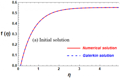
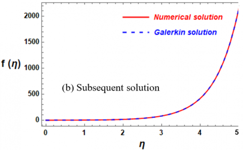
It is worth noting here that the system being dealt with represents a jerk model, which is a nonlinear differential equation. Therefore, it is difficult to obtain an exit solution, so we can conclude that our method maintains an error rate less than $X%$ that of numerical solutions. Although the accuracy of the analytical method used has been previously evaluated in numerous studies in the literature, this is the first time it has been used in such systems, where the boundary conditions contain infinity. Therefore, it was necessary to compare the solution obtained using Galerkin method with numerical solutions using the most reliable and common method for this type of problem, the shooting method. This is illustrated graphically in Figures 2(a), 2(b), 3(a), and 3(b). In addition, the error in the calculations between the numerical and analytical solutions is calculated in Tables 1 and 2 to demonstrate the extent of agreement between the results and provide confidence in the analytical method used for this type of fluid flow system. Figure 2(a) represents a comparison between the numerical and Galerkin initial solutions for the function $f\left( \eta \right)$. In this a (Galerkin) analytic solution (represented by the dashed blue line), whereas a numerical solution (represented by the solid red line). The solution $f\left( \eta \right)$ is represented on the vertical axis, spanning from 0 to above 0.6, in relation to the independent variable $\eta $ on the horizontal axis, which extends from 0 to 5. The great agreement between the Galerkin and Numerical solutions over the whole region of $\eta $ displayed is a remarkable aspect of this study. The answers are identical, as seen by the nearly perfect superimposition of the blue dashed line (Galerkin) and the red solid line (shooting). Furthermore, low $\eta $ Values ($\eta \simeq 0$ to $\eta \simeq 2$) are indicated by this diagram: The function f(η) shows a fast, non-linear exponential-like growth as $\eta $ grows, reaching values between 0 and 0.5 at $\eta \simeq 2$. The superposition of the two curves is preserved even in this area of significant amplitude and fast change. In the second case (subsequent solution), Figure 2(b) also shows a comparison between the numerical and the initial Galerkin solutions for the function $f\left( \eta \right)$. The vertical axis, which spans from 0 to over 2000, represents the function $f\left( \eta \right)$, while the horizontal axis, which spans from 0 to 5, represents the independent variable $\eta $. The function $f\left( \eta \right)$ exhibits rapid nonlinear growth with the growth of $\eta $. The high agreement between the Galerkin and numerical solutions, represented in blue and red, remains prominent throughout the entire range, even in this region of rapid change. Compared favorably to the numerical solution, this is an important observation that shows how accurate and robust the Galerkin approach is at capturing complex, high-magnitude non-linear phenomena.
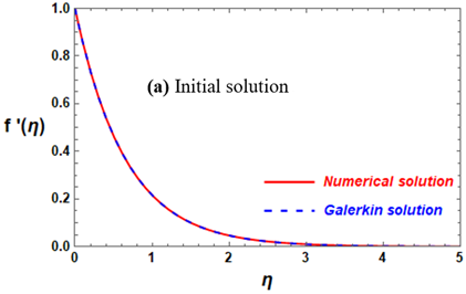
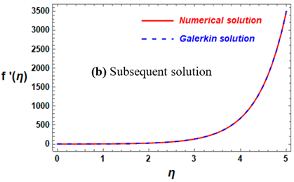
Additionally, Figure 3(a) and Figure 3(b) show comparisons of the numerically calculated and analytically calculated velocities $f'\left( \eta \right)$. This effective comparison, which clearly demonstrates the overlap between the analytically calculated velocity curves and their numerically calculated counterparts, is an important result that demonstrates the accuracy and robustness of the Galerkin technique in capturing the complex, high-volume nonlinear phenomena that occur in magneto-fluid flow problems in porous media. This technique has numerous applications in diverse fields, including hydrogeology (groundwater flow), petroleum engineering (oil and gas reservoir modeling), biomedical engineering (flow in biological tissues), and industrial applications (filters and heat exchangers).
Figure 2. A comparison between the Galerkin and numerical solutions for $f\left( \eta \right)$ at $\alpha =K=1,{{f}_{w}}=-0.1$, and $M=0.5$
Table 1 and Table 2 show the percentage of error resulting from comparing the outcomes of the solution $f\left( \eta \right)$ which was calculated analytically via Galerkin’s approach (23) and numerically using the well-known shooting technique for various values of $\eta $ at $K=1,~{{f}_{w}}=-0.1$, and $M=0.5$. The number of relative errors between the results of the two methods, whether in the first or second solution, is within a part per million, which expresses the accuracy of Galerkin’s strategy. The strong relationship supports the Galerkin method's usage as a trustworthy supplement or substitute for the numerical solution to this problem. The Galerkin method, a kind of weighted residual approach frequently used to discover approximate solutions to differential equations, appears to be successfully convergent to the genuine solution (represented here by the Numerical result) based on the minimal variation between the two solutions. When an analytical approximation is preferred over a purely numerical method, or for further study, these figures and tables effectively illustrate the excellent accuracy of the Galerkin solution and its safe use.
Figure 3. A comparison of the Galerkin and computational answers for $df/d\eta $ at $K=1,{{f}_{w}}=-0.1$, and $M=0.5$
Table 1. Relative error between the Galerkin and numerical first solution $f\left( \eta \right)$ for various values of $\eta $ at $K=1,{{f}_{w}}=-0.1$, and $M=0.5$
|
$\eta $ |
First Solution |
||
|
Galerkin’s Method Solution |
Computational Solution |
Percentage Error |
|
|
0.2 |
0.0782245 |
0.0782244 |
9.6 $\times {{10}^{-7}}$ |
|
0.4 |
0.219102 |
0.219102 |
1.4 $\times {{10}^{-6}}$ |
|
0.6 |
0.330459 |
0.330458 |
2.1 $\times {{10}^{-6}}$ |
|
0.8 |
0.418480 |
0.418479 |
3.0 $\times {{10}^{-6}}$ |
|
1.0 |
0.488057 |
0.488055 |
1.1 $\times {{10}^{-6}}$ |
|
1.2 |
0.543054 |
0.543051 |
5.2 $\times {{10}^{-6}}$ |
|
1.4 |
0.586527 |
0.586523 |
6.5 $\times {{10}^{-6}}$ |
|
1.6 |
0.620889 |
0.620884 |
7.9 $\times {{10}^{-6}}$ |
|
1.8 |
0.648051 |
0.648045 |
9.5 $\times {{10}^{-6}}$ |
|
2.0 |
0.669522 |
0.669514 |
1.1 $\times {{10}^{-5}}$ |
4.2 Computational illustrations
Fractal parameters provide a sophisticated, physically realistic way to characterize the microstructure of the porous medium. This characterization then feeds directly into the governing equations (like the momentum equation via permeability/drag) and indirectly affects the MHD-specific terms (like the Lorentz force) and transport phenomena (like heat and mass transfer), leading to distinct flow behaviors compared to idealized, non-fractal porous media models. Therefore, this discussion section interprets the stream function $\psi \left( x,y \right)$ (25) plot under the effect of fractal parameters $\alpha ~$and $\beta $, links the visual data to fundamental fluid mechanics concepts (velocity gradient). All calculations in this section have been done at $K=1,{{f}_{w}}=-0.1,M=0.5$, and $c=\nu =1$. The analytical results obtained from Galerkin’s approach, particularly the visualization of the stream function $\psi $ in Figures 4, 5, 6, and 7, provide clear insights into the development and characteristics of the internal fluid flow. The stream function contours represent the instantaneous streamlines of the flow, thereby elucidating both the qualitative flow patterns and the underlying velocity distribution.
Table 2. Relative error between the Galerkin and numerical second solution $f\left( \eta \right)$ for various values of $\eta $ at $K=1,{{f}_{w}}=-0.1$, and $M=0.5$
|
$\eta $ |
First Solution |
||
|
Galerkin’s Method Solution |
Computational Solution |
Percentage Error |
|
|
0.2 |
0.127831 |
0.127832 |
6.3 $\times {{10}^{-6}}$ |
|
0.4 |
0.421884 |
0.421886 |
4.9 $\times {{10}^{-6}}$ |
|
0.6 |
0.801405 |
0.801409 |
4.8 $\times {{10}^{-6}}$ |
|
0.8 |
1.29124 |
1.29124 |
4.8 $\times {{10}^{-6}}$ |
|
1.0 |
1.92344 |
1.92345 |
4.9 $\times {{10}^{-6}}$ |
|
1.2 |
2.73941 |
2.73942 |
4.8 $\times {{10}^{-6}}$ |
|
1.4 |
3.79254 |
3.79256 |
4.7 $\times {{10}^{-6}}$ |
|
1.6 |
5.15177 |
5.15180 |
4.5 $\times {{10}^{-6}}$ |
|
1.8 |
6.90608 |
6.90611 |
4.3 $\times {{10}^{-6}}$ |
|
2.0 |
9.17029 |
9.17033 |
4.0 $\times {{10}^{-6}}$ |
For the first solution, Figure 4 illustrates the impact of fractal parameter $\alpha $ on the stream function. Figure 4 clearly illustrates the development of the velocity profile over the stretching surface, in the range from $y=0$ and $y=3$. The contours corresponding to different $\psi \left( x,y \right)$ values are observed to be nearly parallel to the $x$-axis throughout the domain, confirming that the flow is predominantly unidirectional in the $x$-direction, in the range from $x=0$ and $x=10$. A crucial finding is the non-uniform spacing between the streamlines. According to fluid dynamics principles, the distance between adjacent streamlines is inversely proportional to the local flow velocity. A tight clustering of streamlines signifies high velocity, while wider spacing indicates slower movement. With decreasing the magnitude of $\alpha $, a decrease in the magnitude of the stream expression $\psi \left( x,y \right)$ is observed at a constant value for fractal parameter ($\beta =1$). For the second solution, Figure 5 also represents that as the magnitude of $\alpha $, a reduction in the magnitude of the stream function $\psi $ has occurred. However, comparing the results in the two cases in Figures 4 and 5, it can be observed that the impact of the fractal parameter$~\alpha $ on the stream function $\psi ~$in the second case is significantly greater than in the first case with the same constant parameters $K,{{f}_{w}},M$, and $\beta $.
On the other hand, Figures 6 and 7 demonstrate the influence of the fractal factor ($\beta $) regarding the behavior of the stream function $\psi $, both in first and second solutions, respectively, at a constant value of fractal parameter ($\alpha =1$). The shape of the curvature of the stream function $\psi $ gradually decreases and becomes smoother with increasing $\beta $, reaching a value of unity, which represents a continuous space state. This observation is more evident in the initial solution's case than in the subsequent solution's case. Consequently, by studying the effect of these fractal parameters on the stream function, we find that they have a significant impact on the fluid flow behavior. This demonstrates the effectiveness of incorporating the study of the effect of these parameters on movement and, subsequently, the investigation of motion in a fractal space.
In summary, the above Figures indicate that if the fractal parameter takes a value of unity (the normal case in which there are no fractals), the flow function reaches its highest value. That is, fractals function as forces resisting flow, similar in effect to the forces of the porous medium.
(a) $\alpha =0.5$
(b) $\alpha =0.7$
(c) $\alpha =1$
Figure 4. The influence of the concerning fractal factor $\alpha $ upon the stream function $\psi \left( x,y \right)$ (initial solution) at $K=1,{{f}_{w}}=-0.1,M=0.5$, and $\beta =1$
(a) $\alpha =0.5$
(b) $\alpha =0.7$
(c) $\alpha =1$
Figure 5. The influence of the concerning fractal factor $\alpha $ upon the stream function $\psi \left( x,y \right)$ (subsequent solution) at $K=1,{{f}_{w}}=-0.1,M=0.5$, and $\beta =1$
(a) $\beta =0.5$
(b) $\beta =0.7$
(c) $\beta =1$
Figure 6. The influence of the concerning fractal factor $\beta $ upon the stream function $\psi \left( x,y \right)$ (initial solution) at $K=1,{{f}_{w}}=-0.1,M=0.5$, and $\alpha =1$
(a) $\beta =0.5$
(b) $\beta =0.7$
(c) $\beta =1$
Figure 7. The influence of the concerning fractal factor $\beta $ upon the stream function $\psi \left( x,y \right)$ (subsequent solution) at $K=1,{{f}_{w}}=-0.1,M=0.5$, and $\alpha =1$
Dimension or scale is a fundamental issue when studying a problem. Various scales can provide various outcomes when one observes something. Two scales can be employed to address the most practical issues, and for handling discontinuous issues, an updated definition of a dual-scale dimension is presented in place of the fractal dimension. Although the dual-scale theory views every issue with dual scales - the big one for an approximate smooth problem where the classical calculus can be applied fully, in one case, the impact of regarding the porous structure's effect on the characteristics can be described. In this paper, we aim to derive dual analytical solutions for nonlinear fractional MHD models using dual-scale transformation and Galerkin’s approach, then verify them against numerical results. The proposed strategy can be summarized as follows:
Fractals act as forces resisting flow, similar in effect to the forces of the porous medium.
|
$c$ |
positive constant, s-1 |
|
$\left( u,v \right)$ |
velocity components along the $x$ and $y$ axes, m·s-1 |
|
$\left( x,y \right)$ |
cartesian coordinates along the surface and normal to it |
|
${{B}_{0}}$ |
magnetic field strength, kg‧m-2·s-1 |
|
$k$ |
permeability, m2 |
|
$\left( {{x}_{0}},{{y}_{0}} \right)$ |
lowest hierarchical $x$ and $y$ levels |
|
$M$ |
dimensionless magnetic parameter |
|
$K$ |
dimensionless permeability parameter |
|
${{f}_{w}}$ |
dimensionless mass transfer parameter, positive/negative sign for injection/suction |
|
$\left( X,Y \right)$ |
dual-scale transformation |
|
$\left( {{u}_{w}},{{V}_{w}} \right)$ |
horizontal and vertical velocities at the sheet, m·s-1 |
|
$R$ |
residual function |
|
${{C}_{~f}}$ |
coefficient of local skin fraction |
|
$R{{e}_{X}}$ |
Reynolds number at a local point |
|
Greek symbols |
|
|
$\left( \alpha ,\beta \right)$ |
fractal dimension parameters |
|
$\rho $ |
fluid density, kg·m-3 |
|
$\sigma $ |
electrical conductivity, m-1·s |
|
$\nu $ |
kinematic viscosity, m2·s-1 |
|
$\mu $ |
dynamic viscosity, (Pa‧s) kg. m-1·s-1 |
|
$\eta $ |
similarity variable |
|
$\psi $ |
stream function |
|
${{\tau }_{w}}$ |
shear stress |
[1] Kabeel, A.E., El-Said, E.M., Dafea, S.A. (2015). A review of magnetic field effects on flow and heat transfer in liquids: Present status and future potential for studies and applications. Renewable and Sustainable Energy Reviews, 45: 830-837. https://doi.org/10.1016/j.rser.2015.02.029
[2] Polo, J., Mackay, T., Lakhtakia, A. (2013). Electromagnetic Surface Waves: A Modern Perspective. Elsevier Inc. https://doi.org/10.1016/C2011-0-07510-5
[3] Huang, Z., Li, Z. (2000). The fractal dimension and fractal interval for freeway traffic flow. ITSC2000. 2000 IEEE Intelligent Transportation Systems, Proceedings, Dearborn, USA, pp. 1-4. https://doi.org/10.1109/ITSC.2000.881008
[4] Peli, T. (1990). Multiscale fractal theory and object characterization. Journal of the Optical Society of America A, 7(6): 1101-1112. https://doi.org/10.1364/JOSAA.7.001101
[5] Wang, K. (2021). A new fractal model for the soliton motion in a microgravity space. International Journal of Numerical Methods for Heat and Fluid Flow, 31(1): 442-451. https://doi.org/10.1108/HFF-05-2020-0247
[6] Tatekawa, T., Maeda, K.I. (2001). Primordial fractal density perturbations and structure formation in the universe: One-dimensional collisionless sheet model. The Astrophysical Journal, 547(2): 531-544. https://doi.org/10.3389/fphy.2019.00081
[7] Kumar, D., Baleanu, D. (2019). Fractional calculus and its applications in physics. Frontiers in Physics, 7: 81. https://doi.org/10.3399/978-2-88945-958-2
[8] Zhang, Y., Sun, H., Stowell, H.H., Zayernouri, M., Hansen, S.E. (2017). A review of applications of fractional calculus in Earth system dynamics. Chaos, Solitons and Fractals, 102: 29-46. https://doi.org/10.1016/j.chaos.2017.03.051
[9] Simpson, R., Jaques, A., Nuñez, H., Ramirez, C., Almonacid, A. (2013). Fractional calculus as a mathematical tool to improve the modeling of mass transfer phenomena in food processing. Food Engineering Reviews, 5(1): 45-55. https://doi.org/10.1007/s12393-012-9059-7
[10] Stanislavsky, A.A. (2010). Astrophysical applications of fractional calculus. Proceedings of the Third UN/ESA/NASA Workshop on the International Heliophysical Year 2007 and Basic Space Science: National Astronomical Observatory of Japan, pp. 63-78. https://doi.org/10.1007/978-3-642-03325-4_8
[11] Nonnenmacher, T.F., Metzler, R. (2000). Applications of fractional calculus techniques to problems in biophysics. Applications of Fractional Calculus in Physics, pp. 377-427. https://doi.org/10.1142/3779
[12] Li, J., Ostoja-Starzewski, M., Tarasov, V.E. (2019). Application of fractional calculus to fractal media. Applications in Physics, Part A, pp. 263-276. https://doi.org/10.1515/9783110571707-011
[13] Tarasov, V.E. (2011). Fractional dynamics: Applications of fractional calculus to dynamics of particles, fields and media. Springer Science and Business Media. https://link.springer.com/10.1007/978-3-642-14003-7
[14] Elgazery, N.S. (2020). A periodic solution of the Newell-Whitehead-Segel (NWS) wave equation via fractional calculus. Journal of Applied and Computational Mechanics, 6: 293-1300. https://doi.org/10.22055/JACM.2020.33778.2285
[15] El-Dib, Y.O., Elgazery, N.S., Khattab, Y.M., Alyousef, H.A. (2023). An innovative technique to solve a fractal damping Duffing-jerk oscillator. Communications in Theoretical Physics, 75(5): 055001. https://doi.org/10.1088/1572-9494/acc646
[16] El-Dib, Y., Elgazery, N.S., Alyousef, H.A. (2024). The up-grating rank approach to solve the forced fractal Duffing oscillator by non-perturbative technique. Facta Universitatis, Series: Mechanical Engineering, pp. 199-216. https://doi.org/10.22190/FUME230605035E
[17] Wu, P.X., Ling, W.W., Li, X.M., Xie, L.J. (2021). Variational principle of the one-dimensional convection–dispersion equation with fractal derivatives. International Journal of Modern Physics B, 35(19): 2150195. https://doi.org/10.1142/S0217979221501952
[18] Feng, G.Q. (2021). He’s frequency formula to fractal undamped Duffing equation. Journal of Low Frequency Noise, Vibration and Active Control, 40(4): 1671-1676. https://doi.org/10.1177/1461348421992608
[19] Ain, Q.T., Anjum, N., He, C.H. (2021). An analysis of time-fractional heat transfer problem using two-scale approach. GEM-International Journal on Geomathematics, 12(1): 18. https://doi.org/10.1007/s13137-021-00187-x
[20] Nadeem, M., He, J.H. (2022). The homotopy perturbation method for fractional differential equations: Part 2, two-scale transform. International Journal of Numerical Methods for Heat and Fluid Flow, 32(2): 559-567. https://doi.org/10.1108/HFF-01-2021-0030
[21] Ain, Q.T., He, J.H. (2019). On two-scale dimension and its applications. Thermal Science, 23(3 Part B): 1707-1712. https://doi.org/10.2298/TSCI190408138A
[22] Li, Z.B., Zhu, W.H., He, J.H. (2012). Exact solutions of time-fractional heat conduction equation by the fractional complex transform. Thermal Science, 16(2): 335-338. https://doi.org/10.2298/TSCI110503069L
[23] He, J.H., Ain, Q.T. (2020). New promises and future challenges of fractal calculus: From two-scale thermodynamics to fractal variational principle. Thermal Science, 24(2 Part A): 659. https://doi.org/10.2298/TSCI200127065H
[24] Tian, D., Ain, Q.T., Anjum, N., He, C.H., Cheng, B. (2021). Fractal N/MEMS: From pull-in instability to pull-in stability. Fractals, 29(2): 2150030. https://doi.org/10.1142/S0218348X21500304
[25] Tian, D., He, C.H., He, J.H. (2021). Fractal pull-in stability theory for microelectromechanical systems. Frontiers in Physics, 9: 606011. https://doi.org/10.3389/fphy.2021.606011
[26] Liu, H., Yao, S.W., Yang, H., Liu, J. (2019). A fractal rate model for adsorption kinetics at solid/solution interface. Thermal Science, 23(4): 2477-2480. https://doi.org/10.2298/TSCI1904477L
[27] Wang, K. (2021). A new fractal model for the soliton motion in a microgravity space. International Journal of Numerical Methods for Heat and Fluid Flow, 31(1): 442-451. https://doi.org/10.1108/HFF-05-2020-0247
[28] Zuo, Y. (2021). A gecko-like fractal receptor of a three-dimensional printing technology: A fractal oscillator. Journal of Mathematical Chemistry, 59(3): 735-744. https://doi.org/10.1007/s10910-021-01212-y
[29] Elias-Zuniga, A., Palacios-Pineda, L.M., Jimenez-Cedeno, I.H., Martinez-Romero, O., Olvera-Trejo, D. (2021). A fractal model for current generation in porous electrodes. Journal of Electroanalytical Chemistry, 880: 114883. https://doi.org/10.1016/j.jelechem.2020.114883
[30] Elias-Zuniga, A., Palacios-Pineda, L.M., Jimenez-Cedeno, I.H., Martinez-Romero, O., Olvera-Trejo, D. (2021). Analytical solution of the fractal cubic-quintic Duffing equation. Fractals, 29(4): 2150080. https://doi.org/10.1142/S0218348X21500808
[31] He, C. H., Liu, C., He, J.H., Gepreel, K.A. (2021). Low frequency property of a fractal vibration model for a concrete beam. Fractals, 29(5): 2150117. https://doi.org/10.1142/S0218348X21501176
[32] Wang, K.L., Wei, C.F. (2021). A powerful and simple frequency formula to nonlinear fractal oscillators. Journal of Low Frequency Noise, Vibration and Active Control, 40(3): 1373-1379. https://doi.org/101177/1461348420947832
[33] Deppman, A., Megías, E., Pasechnik, R. (2023). Fractal derivatives, fractional derivatives and q-deformed calculus. Entropy, 25(7): 1008. https://doi.org/10.3390/e25071008
[34] He, J.H., Ji, F.Y. (2019). Two-scale mathematics and fractional calculus for thermodynamics. Thermal Science, 23(4): 2131-2133. https://doi.org/10.2298//TSCI1904131H
[35] Elbarbary, E.M., Elgazery, N.S. (2004). Chebyshev finite difference method for the effect of variable viscosity on magneto-micropolar fluid flow with radiation. International Communications in Heat and Mass Transfer, 31(3): 409-419. https://doi.org/10.1016/j.icheatmasstransfer.2004.02.011
[36] Elshehawey, E.F., Eldabe, N.T., Elbarbary, E.M., Elgazery, N.S. (2004). Chebyshev finite-difference method for the effects of Hall and ion-slip currents on magneto-hydrodynamic flow with variable thermal conductivity. Canadian Journal of Physics, 82(9): 701-715. https://doi.org/10.1139/p04-038
[37] Eldabe, N.T., Elshehawey, E.F., Elbarbary, E.M., Elgazery, N.S. (2005). Chebyshev finite difference method for MHD flow of a micropolar fluid past a stretching sheet with heat transfer. Applied Mathematics and Computation, 160(2): 437-450. https://doi.org/10.1016/j.amc.2003.11.013
[38] El-Dib, Y.O., Elgazery, N.S., Alyousef, H.A. (2023). Galerkin’s method to solve a fractional time-delayed jerk oscillator. Archive of Applied Mechanics, 93(9): 3597-3607. https://doi.org/10.1007/s00419-023-02455-8
[39] Al-Arabi, T.H., Elgazery, N.S. (2024). Photocatalysis case study of wastewater treatment using magneto-radiative Williamson tri-hybrid nanofluid. Case Studies in Thermal Engineering, 60: 104715. https://doi.org/10.1016/j.csite.2024.104715
[40] Abu-Hamdeh, N.H., Basem, A., AL-bonsrulah, H.A., Khoshaim, A., Albdeiri, M.S., Alghawli, A.S. (2024). Galerkin method for simulating the solidification of water in existence of nano-powders. Journal of Thermal Analysis and Calorimetry, 149: 14163-14174. https://doi.org/10.1007/s10973-024-13740-1
[41] Moatimid, G.M., Elgazery, N.S., Mohamed, M.A., Elagamy, K. (2025). Magneto-blood ternary-hybrid nanofluid flow with microorganisms near a vertical plate: Prandtl prototype. Journal of Porous Media, 28(12): 81-119. https://doi.org/10.1615/JPorMedia.2025056655