Perumal Rajan Sakthivel*![]() | Lakshminathan Sivakami
| Lakshminathan Sivakami![]()
© 2025 The authors. This article is published by IIETA and is licensed under the CC BY 4.0 license (http://creativecommons.org/licenses/by/4.0/).
OPEN ACCESS
To date, numerous studies have been conducted on non-Newtonian fluids under various parameters, and their results have been documented and applied in many fields. This study investigates the changes in the MHD Casson fluid by the Laplace transform technique for multi-parameter coupling, such as pressure, heat source, chemical reaction, thermal reaction, etc., under the Dufour effect. The experiment considers a fast-moving plate, where the flow is confined to $x>0$, normal to the surface under fixed boundary conditions, and records the output. Analytically, the PDEs are solved, and the results are supported by the graphs conjoined using MATLAB. The output of the study is that the pressure is inversely proportional to velocity, and the Dufour effect is directly proportional to both velocity and temperature.
Dufour effect, heat source, Laplace transform, MHD, pressure gradient
Casson fluid has a wide range of applications across various practical and industrial sectors. Casson [1] established the flow model for pigment-oil dispersion, the ink used to print. The Casson fluid model better fits rheological properties for several materials. Alam [2] conducted an evaluation of the limitations of heat generation/absorption, Thermomigration, and transfer of mass, within the boundary layer’s movement via a leaning permeable sheet that stretches. Lone et al. [3] tested the layered flow of a non-Newtonian Casson fluid, which involves microbes on a stretchable plane along with activation energy. Silva et al. [4] looked into the magnetohydrodynamic dynamics of a Newtonian suspension utilizing the Laplace transform. Tai and Char [5] did a simulation on the impacts of thermal-diffusion and diffusion-thermo via the transmission of mass and heat in the independent convection flow of non-Newtonian solution along a straight line in a poriferous substrate, incorporating thermal radiation. Ramudu et al. [6] worked out the effectiveness of Soret and Dufour on the magnetohydrodynamic Casson fluid across an elongated region within convective-diffusive circumstances. Sahu and Deka [7] examined the potential dynamics of heating stratification and synthetic responses on MHD free convective flow in tandem with a propelled lateral board.
Ramalingeswara Rao et al. [8] inspected the radiation absorption effect of an unstable MHD, free convection in a Casson fluid flowing along a substantially indefinite lateral slab within a pory system. Živojin et al. [9] executed an analysis of the MHD flow involving a pair of insoluble solutions, while integrating potential effects of an applied electric field and a tilted magnetic field.
Jalili et al. [10] deduced the impact of thermo-diffusion, electric waves, and nonlinear heat rays. Swetha et al. [11] assessed the radiation and Soret effects on a floundering convective stream characterized by mass and heat displacement of incompressible substance over a level surface situated in a highly pervious base. Kataria and Patel [12] calculated the roles of thermal diffusion with heat creation upon the circulation of an MHD Casson fluid over a swaying straightened platter set inside a porous structure, while recording the output in account of chemical and thermal reactions. Mahboobtosi et al. [13] executed a research endeavour examining the influence of several parameters, such as the Schmidt quantity, Prandtl dosages, and permeation value, on the magnitude of acceleration, temp, and concentration. Turkyilmazoglu and Pop [14] handled an analytical validation of the mass migration and heat relevant to the erratic movement of a fluid with a capacity for electricity via a swiftly set up straight unlimited erect plat.
Sivakami et al. [15] examined factors including mass exchange, chemical responses, and energy sources, in addition to the control of Dufour on certain MHD concentric inert flow patterns in a straight path. A study by Yesodha et al. [16] examined the changes in the Soret and Dufour factors as well, the characteristics of heat transmission, mass transfer, and activation energy transfer for a reaction product in a viscous fluid in a concentric frame. Jiang et al. [17] validated the work by considering a comprehensive physical model that incorporates all coupling effects. Sheri et al. [18] measured the swinging of Hall Current, Dufour, and Soret effects on fluent flow concerning the slanted permeable surface. Sakthivel and Sivakami [19] predicted the result of the same model without the pressure medium, and in this current scenario, we have extended it to other metrics also. Bekezhanova and Goncharova [20] examined the Soret measure in the scenario for the vapor concentration and estimated the dosages based on the warmth stress and inclusion/exclusion of the thermos diffusion factor.
Where the previous studies haven’t systematically examined the pressure gradient interaction with the Dufour effect. This paper aims to study the Dufour effects on the Casson fluid flow, considering the pressure, heat source, chemical reaction, and various other parameters. Here in Section 2, we have done the mathematical formulation and worked out the solution. Section 3 examines the possibilities of varying many parameters, including velocity, temperature, and concentration gradients.
This study examines an unstable Casson fluid in motion in front of an accelerated plate, with the motion restricted to the region where to $x>0$, where x indicates the normal to the surface. At the earliest time t = 0, the plate moves in tandem with the fluid, maintaining identical concentration and temperature levels. The plate reaches a velocity of $u^{\prime}=A t$ when $t>0$, as the concentration C' and temperature T' of the plate are changed to $T_W^{\prime}$ and $C_W^{\prime}$.
The subsequent dimensional momentum, energy, and concentration equations regulate the flow:
$\rho \frac{\partial u^{\prime}}{\partial t^{\prime}}=\mu\left(1+\frac{1}{\gamma}\right) \frac{\partial^2 u^{\prime}}{\partial x^{\prime 2}}+\rho g \beta^{\prime\left(T^{\prime}-T_{\infty}^{\prime}\right)}-\sigma B_0^2 u^{\prime}-\frac{v}{K} u^{\prime}+\rho g \beta^*\left(C^{\prime}-C_{\infty}^{\prime}\right)+\frac{\partial p^{\prime}}{\partial x^{\prime}}$ (1)
$\rho C_P \frac{\partial T^{\prime}}{\partial t^{\prime}}=k \frac{\partial^2 T^{\prime}}{\partial x^{\prime 2}}+\frac{D_m K_T}{C_S} \frac{\partial^2 C^{\prime}}{\partial x^{\prime 2}}-Q_s\left(T^{\prime}-T_{\infty}\right)$ (2)
$\rho C_P \frac{\partial C^{\prime}}{\partial t^{\prime}}=D \frac{\partial^2 C^{\prime}}{\partial x^{\prime 2}}-K r^{\prime}\left(C^{\prime}-C^{\prime}{ }_{\infty}\right)$ (3)
With the earliest and confined conditions
$\begin{aligned} & u^{\prime}\left(x^{\prime}, 0\right)=0 ; \quad u^{\prime}\left(0, t^{\prime}\right)=A t ; \quad u^{\prime}\left(\infty, t^{\prime}\right)=0 ; \\ & T^{\prime}\left(x^{\prime}, 0\right)=T_{\infty}^{\prime} ; T^{\prime}\left(0, t^{\prime}\right)=T_w^{\prime} ; T^{\prime}\left(\infty, t^{\prime}\right)=T_{\infty}^{\prime} ; \\ & C^{\prime}\left(x^{\prime}, 0\right)=C_{\infty}^{\prime} ; C^{\prime}\left(0, t^{\prime}\right)=C_w^{\prime} ; C^{\prime}\left(\infty, t^{\prime}\right)=C_{\infty}^{\prime} ;\end{aligned}$ (4)
And by calculating non-dimensional quantities (1), (2), and (3) turn into dimensionless form:
$\begin{gathered}u=\frac{u^{\prime}}{(v A)^{\frac{1}{3}}}, t=\frac{t^{\prime A^{\frac{2}{3}}}}{v^{\frac{1}{3}}}, x=\frac{x^{\prime A^{\frac{1}{3}}}}{v^{\frac{2}{3}}}, T=\frac{T^{\prime}-T_{\infty}^{\prime}}{T_W^{\prime}-T_{\infty}^{\prime}}, C=\frac{C^{\prime}-C_{\infty}^{\prime}}{C_W^{\prime}-C_{\infty}^{\prime}}, M=\frac{\sigma B_0^2 v^{\frac{1}{3}}}{\rho A^{\frac{2}{3}}}, N=\frac{16 \sigma T_{\infty}}{3 k}, \operatorname{Pr}=\frac{\mu C_\rho}{k}, A=1+\frac{1}{\gamma}, \mu=\rho v, \\ G r=\frac{g \beta^{\prime}\left(T_W^{\prime}-T_{\infty}^{\prime}\right)}{A}, G c=\frac{g \beta^*\left(C_W^{\prime}-C_{\infty}^{\prime}\right)}{A}, D_f=\frac{D_m K_T\left(C_W^{\prime}-C_{\infty}^{\prime}\right)}{v C_S C_\rho\left(T_W^{\prime}-T_{\infty}^{\prime}\right)}, B=M+\frac{1}{k}, \lambda=\frac{P r}{1+N}, S_c=\frac{v}{D};\end{gathered}$ (5)
Now, by using the above parameters in (1)-(3). We will be able to get the dimensionless form of those equations, which are given by Eqs. (6)-(8).
$\frac{\partial u}{\partial t}=A \frac{\partial^2 u}{\partial x^2}+G r T-B u+G c C+p$ (6)
$\lambda \frac{\partial T}{\partial t}=\frac{\partial^2 T}{\partial x^2}-Q T+D_f \frac{\partial^2 C}{\partial x^2}$ (7)
$\frac{\partial C}{\partial t}=\frac{1}{S c} \frac{\partial^2 C}{\partial x^2}-K r C$ (8)
With earliest and confined conditions:
$\begin{aligned} & u(x, 0)=0 ; u(0, t)=a t ; u(\infty, t)=0 ; \\ & \mathrm{T}(x, 0)=0 ; T(0, t)=1 ; T(\infty, t)=0 ; \\ & C(x, 0)=0 ; c(0, t)=1 ; C(\infty, t)=0 ;\end{aligned}$ (9)
The analytical solution is done using the Laplace Transform:
$\frac{\partial^2 \bar{U}}{\partial x^2}+\frac{(s+B)}{A} \bar{U}=-R_1 \bar{T}-R_2 \bar{C}-R_3 \frac{1}{s}$ (10)
$\frac{\partial^2 \bar{T}}{\partial x^2}-\lambda s \bar{T}-Q \bar{T}=-D u \frac{\partial^2 \bar{C}}{\partial x^2}$ (11)
$\frac{\partial^2 \bar{C}}{\partial x^2}-\bar{C}(S c K r+S c s)=0$ (12)
where, the parameters used are:
$R_1=\frac{G r}{A}, R_2=\frac{G c}{A}, R_3=\frac{p}{A}, D_f=D u$
The inverse Laplace tactic has been implemented to solve (10), (11), and (12).
$C(x, t)=\frac{e^{k r t}}{2}\left\{e^{-x \sqrt{k r S c}} . \operatorname{erfc}\left(\frac{x \sqrt{S c}}{2 \sqrt{t}}-\sqrt{K r t}\right)+e^{x \sqrt{K r S c}} . \operatorname{erfc}\left(\frac{x \sqrt{S c}}{2 \sqrt{t}}+\sqrt{K r t}\right)\right\}$ (13)
$\begin{gathered}T(x, t)=\frac{e^{\frac{Q}{\lambda} t}}{2}\left\{e^{-x \sqrt{Q}} . \operatorname{erfc}\left(\frac{x \sqrt{\lambda}}{2 \sqrt{t}}-\sqrt{\frac{Q}{\lambda} t}\right)+e^{x \sqrt{Q}} . \operatorname{erfc}\left(\frac{x \sqrt{\lambda}}{2 \sqrt{t}}+\sqrt{\frac{Q}{\lambda} t}\right)\right\}+a_1 a_2 k r S c\left\{\frac{e^{\left(k r+\frac{1}{a_1}\right) t}}{2}\left[e^{-x \sqrt{\operatorname{sc}\left(k r+\frac{1}{a_1}\right)}} . \operatorname{erfc}\left(\frac{x \sqrt{\operatorname{Sc}}}{2 \sqrt{t}}-\sqrt{\left(k r+\frac{1}{a_1}\right) t}\right)\right.\right. \\ \left.\left.+e^{x \sqrt{\operatorname{sc}\left(k r+\frac{1}{a_1}\right)}} . \operatorname{erfc}\left(\frac{x \sqrt{\operatorname{Sc}}}{2 \sqrt{t}}+\sqrt{\left(k r+\frac{1}{a_1}\right) t}\right)\right]\right\}\end{gathered}$
$\begin{aligned} & +a_1 S c\left\{\frac{e^{\left(k r+\frac{1}{a_1}\right) t}}{2}\left[e^{-x \sqrt{s c\left(k r+\frac{1}{a_1}\right)}} . \operatorname{erfc}\left(\frac{x \sqrt{S c}}{2 \sqrt{t}}-\sqrt{\left(k r+\frac{1}{a_1}\right) t}\right)+e^{x \sqrt{s c\left(k r+\frac{1}{a_1}\right)}} . \operatorname{erfc}\left(\frac{x \sqrt{S c}}{2 \sqrt{t}}+\sqrt{\left(k r+\frac{1}{a_1}\right) t}\right)\right]\right\} \\ & +a_1 S c\left\{\frac{e^{\left(k r+\frac{1}{a_1}\right) t}}{2}\left[e^{-x \sqrt{s c\left(k r+\frac{1}{a_1}\right)}} . \operatorname{erfc}\left(\frac{x \sqrt{S c}}{2 \sqrt{t}}-\sqrt{\left(k r+\frac{1}{a_1}\right) t}\right)+e^{x \sqrt{s c\left(k r+\frac{1}{a_1}\right)}} . \operatorname{erfc}\left(\frac{x \sqrt{S c}}{2 \sqrt{t}}+\sqrt{\left(k r+\frac{1}{a_1}\right) t}\right)\right]\right\}\end{aligned}$
$\begin{gathered}+a_1 a_2 \lambda Q\left\{\frac{e^{Q t}}{2}\left[e^{-x \sqrt{\lambda Q}} \cdot \operatorname{erfc}\left(\frac{x \sqrt{\lambda}}{2 \sqrt{t}}-\sqrt{Q t}\right)+e^{x \sqrt{\lambda Q}} \cdot \operatorname{erfc}\left(\frac{x \sqrt{\lambda}}{2 \sqrt{t}}+\sqrt{Q t}\right)\right]\right\} \\ -a_1 a_2 \lambda Q\left\{\frac{e^{\left(Q+\frac{1}{a_1}\right) t}}{2}\left[e^{-x \sqrt{\lambda\left(Q+\frac{1}{a_1}\right)}} \cdot \operatorname{erfc}\left(\frac{x \sqrt{\lambda}}{2 \sqrt{t}}-\sqrt{\left(Q+\frac{1}{a_1}\right) t}\right)+e^{x \sqrt{\lambda\left(Q+\frac{1}{a_1}\right)}} \cdot \operatorname{erfc}\left(\frac{x \sqrt{\lambda}}{2 \sqrt{t}}+\sqrt{\left(Q+\frac{1}{a_1}\right) t}\right)\right]\right\}\end{gathered}$
$-a_2 \lambda\left\{\frac{e^{\left(Q+\frac{1}{a_1}\right) t}}{2}\left[e^{-x \sqrt{\lambda\left(Q+\frac{1}{a_1}\right)}} . {erfc}\left(\frac{x \sqrt{\lambda}}{2 \sqrt{t}}-\sqrt{\left(Q+\frac{1}{a_1}\right) t}\right)+e^{x \sqrt{\lambda\left(Q+\frac{1}{a_1}\right)}} . {erfc}\left(\frac{x \sqrt{\lambda}}{2 \sqrt{t}}+\sqrt{\left(Q+\frac{1}{a_1}\right) t}\right)\right]\right\}$ (14)
$-a_1=\frac{S c-\lambda}{S c k r-Q \lambda} ; a_2=\frac{D u}{S c-\lambda} ;$
$\begin{gathered}u(x, t)=a e^{A t}\left\{\left(\frac{t}{2}+\frac{x}{4 \sqrt{A B}}\right) e^{x \sqrt{\frac{B}{A}}} \cdot \operatorname{erfc}\left(\frac{x}{2 \sqrt{A t}}+\sqrt{B t}\right)+\right. \\ \left.\left(\frac{t}{2}-\frac{x}{4 \sqrt{A B}}\right) e^{-x \sqrt{\frac{B}{A}}} \cdot \operatorname{erfc}\left(\frac{x}{2 \sqrt{A t}}-\sqrt{B t}\right)\right\}-R_3\end{gathered}$
$+\frac{K_2}{K_1}\left\{\frac{e^{k r t}}{2}\left[e^{-x \sqrt{S c k r}} . \operatorname{erfc}\left(\frac{x \sqrt{S c}}{2 \sqrt{t}}-\sqrt{k r t}\right)+e^{x \sqrt{S c k r}} . \operatorname{erfc}\left(\frac{x \sqrt{S c}}{2 \sqrt{t}}+\sqrt{k r t}\right)\right]\right\}$
$-\frac{K_2}{K_1}\left\{\frac{e^{\left(k r-K_1\right) t}}{2}\left[e^{-x \sqrt{S c\left(k r-K_1\right)}} . \operatorname{erfc}\left(\frac{x \sqrt{S c}}{2 \sqrt{t}}-\sqrt{\left(k r-K_1\right) t}\right)+e^{x \sqrt{S c\left(k r-K_1\right)}} . \operatorname{erfc}\left(\frac{x \sqrt{S c}}{2 \sqrt{t}}+\sqrt{\left(k r-K_1\right) t}\right)\right]\right\}$
$+\frac{K_4}{K_3}\left\{\frac{e^{Q t}}{2}\left[e^{-x \sqrt{Q \lambda}} \cdot \operatorname{erfc}\left(\frac{x \sqrt{\lambda}}{2 \sqrt{t}}-\sqrt{Q t}\right)+e^{x \sqrt{Q \lambda}} \cdot \operatorname{erfc}\left(\frac{x \sqrt{\lambda}}{2 \sqrt{t}}+\sqrt{Q t}\right)\right]\right\}$
$-\frac{K_4}{K_3}\left\{\frac{e^{\left(Q-K_3\right) t}}{2}\left[e^{-x \sqrt{\left(Q-K_3\right) \lambda}} . \operatorname{erfc}\left(\frac{x \sqrt{\lambda}}{2 \sqrt{t}}-\sqrt{\left(Q-K_3\right) t}\right)+e^{x \sqrt{\left(Q-K_3\right) \lambda}} . \operatorname{erfc}\left(\frac{x \sqrt{\lambda}}{2 \sqrt{t}}+\sqrt{\left(Q-K_3\right) t}\right)\right]\right\}$
$+\frac{K_6 S c k r D u}{K_1}\left\{\frac{e^{K_1 t}}{2}\left[e^{-x \sqrt{S c K_1}} . \operatorname{erfc}\left(\frac{x \sqrt{S c}}{2 \sqrt{t}}-\sqrt{K_1 t}\right)+e^{x \sqrt{S c K_1}} . \operatorname{erfc}\left(\frac{x \sqrt{S c}}{2 \sqrt{t}}+\sqrt{K_1 t}\right)\right]\right\}$
$\begin{aligned} & -\frac{K_6 S c\left(k r-K_1\right) D u}{K_1}\left\{\frac{e^{\left(k r-K_1\right) t}}{2}\left[e^{-x \sqrt{S c\left(k r-K_1\right)}} . \operatorname{erfc}\left(\frac{x \sqrt{S c}}{2 \sqrt{t}}-\sqrt{\left(k r-K_1\right) t}\right)+e^{x \sqrt{S c K_1}} . \operatorname{erfc}\left(\frac{x \sqrt{S c}}{2 \sqrt{t}}+\right.\right.\right. \\ & \left.\left.\left.\sqrt{\left(k r-K_1\right) t}\right)\right]\right\}+\frac{K_6 Q \lambda D u}{K_3}\left\{\frac{e^{Q t}}{2}\left[e^{-x \sqrt{Q \lambda}} . \operatorname{erfc}\left(\frac{x \sqrt{\lambda}}{2 \sqrt{t}}-\sqrt{Q t}\right)+e^{x \sqrt{Q \lambda}} . \operatorname{erfc}\left(\frac{x \sqrt{\lambda}}{2 \sqrt{t}}+\sqrt{Q t}\right)\right]\right\}\end{aligned}$
$-\frac{K_6 \lambda\left(Q-K_3\right) D u}{K_3}\left\{\frac{e^{\left(Q-K_3\right) t}}{2}\left[e^{-x \sqrt{\left(Q-K_3\right) \lambda}} . \operatorname{erfc}\left(\frac{x \sqrt{\lambda}}{2 \sqrt{t}}-\sqrt{\left(Q-K_3\right) t}\right)+e^{x \sqrt{\left(Q-K_3\right) \lambda}} . \operatorname{erfc}\left(\frac{x \sqrt{\lambda}}{2 \sqrt{t}}+\sqrt{\left(Q-K_3\right) t}\right)\right]\right\}$ (15)
$K_1=\frac{A k r S c-B}{A S c-1} ; K_2=\frac{A R_2}{A S c-1} ; K_3=\frac{A Q \lambda-B}{A \lambda-1} ;$
$K_4=\frac{A R_1}{A \lambda-1} ; K_6=\frac{A R_1}{A S c-1}$
The consequence of parameters is calculated, and their effects are observed graphically. From these, we can deduce the outcomes on velocity profile, concentration, and temperature gradients. MATLAB is used for the numerical study of temperature, concentration, and velocity profiles.
3.1 Concentration profile
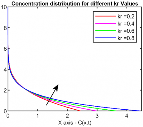
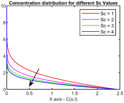
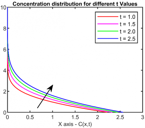
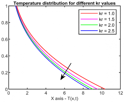
Figures 1 illustrates the link between of chemical response parameters on concentration; as the chemical reaction gains, so does the concentration. Figure 2 illustrates that as the Schmidt number jumps up in values, the concentration gradient drops, and Figure 3 clarifies the times impacts on the concentration, as concentration spikes in correspondence with time.
Figure 1. Response of chemical reaction parameter (Kr) on Concentration for Sc= and t=2
Figure 2. Response of the Schmidt number (Sc) on the Concentration for kr=0.2, t=2
Figure 3. Response of t in Concentration spectrum for Sc=1, kr=0.2
3.2 Temperature profile
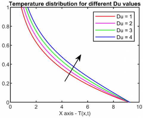
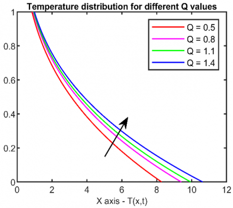
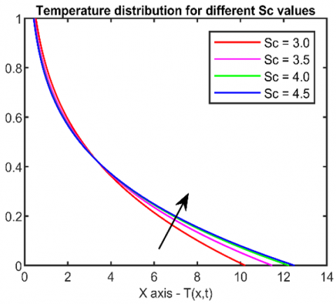
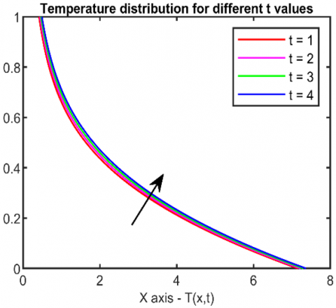
Figure 4 points out that any rise in the Dufour effect translates to the elevation of the temperature field. The Dufour effect is a coupling trend arising from heat flux generated by an applied concentration gradient. A higher value of Du brings about temperatures that are higher across. Figure 5 demonstrates the effete of chemical reaction (kr) on temperature, indicating that a fall in kr brings a decline in temperature. Figure 6 points out the indent of the heat source on temperature. Both are proportional to each other. The rise in heat source is attributed to the rise in temperature. Figure 7 gives the role of Schmidt number (Sc) on temperature, indicating that a climb in the Schmidt number corresponds to rise in temperature. Figure 8 depicts the resultant effect of time (t) over temperature. Over time, the temperature rises gradually.
Figure 4. Response of the Dufour effect (Du) on temperature profile for Q=1, λ=0.5, kr=1.2, Sc=3, t=0.33
Figure 5. Response of the chemical reaction parameter (Kr) on temperature for Q=1, λ=0.5, Du=1, Sc=3, t=0.33
Figure 6. Response of the heat source (Q) on temperature profile for Du=1, λ=0.5, kr=1.2, Sc=3, t=0.33
Figure 7. Response of the Schmidt number (Sc) on the temperature profile for Q=1, λ=0.5, kr=1.2, Du=1, t=0.33
Figure 8. Response of time(t) on temperature profile for Q=1, λ=0.5, kr=1.2, Sc=3, Du=1
3.3 Velocity profile
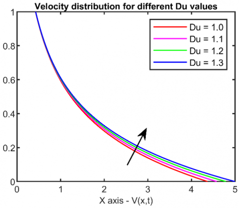
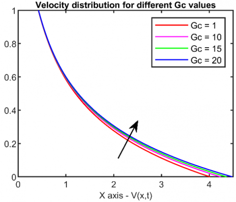
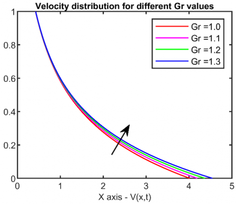
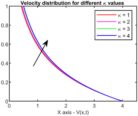
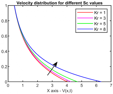
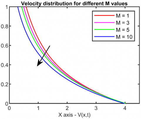
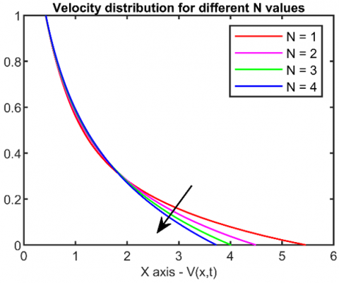
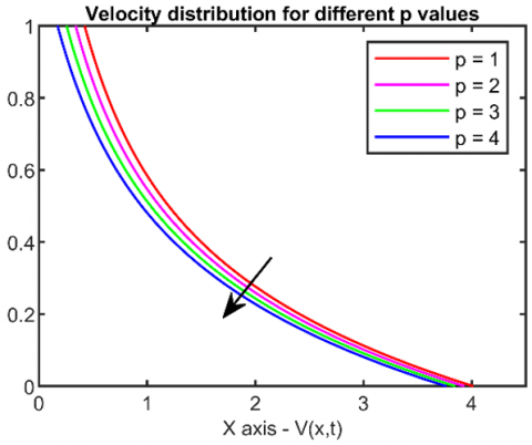
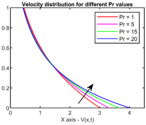
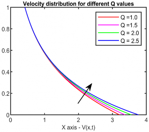
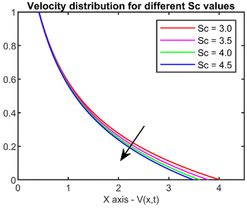
Figure 9 displays that as the Dufour effect (Du) jumps, the velocity profile also rises. Figure 10 illustrates that arise in the mass Grashof number (Gc) corresponds to a boost in the velocity. Any rise in Gc supports the concentration gradient, thereby augmenting the buoyancy forces. this, in turn, enhances fluid flow. Figure 11 gives the resultant that as the thermal Grashof number (Gr) elevates, it contributes to the acceleration of the fluid. Figure 12 illustrates that a growth in permeability k matches the growth in the velocity profile. Darcy's law confirms that the company of a penetrable substance reduces the flow resistance, thereby facilitating movement. Figure 13 reveals that an upsurge in the chemical reaction parameter (Kr) correlates with arise in velocity. Figure 14 gives the role of the Magnetic parameter (M). As the magnitude of the magnetic parameter expands, there is a swift decline in velocity, attributed to the Lorentz force that opposes fluid movement. Figure 15 highlights the negative effect of radiation parameters on velocity. We see that as the N value expands, the velocity gradient reduces. this is because the fluid emits heat to the plate, resulting from the radiation, leading to a lowering of fluid temperature and an upsurge in viscosity. Figure 16 indicates the correspondence between pressure and velocity. As pressure builds up, the velocity diminishes. In Figure 17, we have the effete of the Prandtl number on velocity. We see that as the Prandtl number jumps up, so does the velocity. Figure 18 gives the output of the heat source influence with the velocity profile. As the heat source value moves up, so does the velocity field. In Figure 19, we see how the Schmidt quantity affects the velocity domain. As the Schmidt value is enhanced, we can see a decline in the velocity profile.
Figure 9. Response of the Dufour effect (Du) on the velocity profile with Gr=1, Gc=1, Pr=20, Sc=3, kr=1, k=0.2, M=5, N=3, t=0.33, p =1 gamma=0.2, and Q=4
Figure 10. Response of the mass Grashof number (Gc) on the velocity with Gr=1, Du =1, Pr=20, Sc=3, kr=1, k=0.2, M=5, N=3, t=0.33, p=1, gamma=0.2, and Q=4
Figure 11. Response of the thermal Grashof number (Gr) on the velocity profile with Gc=1, Du =1, Pr=20, Sc=3, kr=1, k=0.2, M=5, N=3, t=0.33, p=1, gamma=0.2, and Q=4
Figure 12. Response of k on the velocity profile with Gr=1, Gc=1, Du =1, Pr=20, Sc=3, kr=1, M=5, N=3, t=0.33, p=1, gamma=0.2, and Q=4
Figure 13. Response of the chemical reaction parameter (Kr) on the velocity. With Gr=1, Gc=1, Du =1, Pr=20, Sc=3, k=0.2, M=5, N=3, t=0.33, p=1, gamma=0.2, and Q=4
Figure 14. Response of the Magnetic parameter (M) on the velocity profile with Gr=1, Gc=1, Du =1, Pr=20, Sc=3, Kr=1, k=0.2, M=5, N=3, t=0.33, p=1, gamma=0.2, and Q=4
Figure 15. Response of the N on the Velocity profile with Gr=1, Gc=1, Du =1, Pr=20, Sc=3, Kr=1, k=0.2, M=5, t=0.33, p=1, gamma=0.2, and Q=4
Figure 16. Response of the pressure gradient (p) on the velocity with Gr=1, Gc=1, Du =1, Pr=20, Sc=3, Kr=1, k=0.2, M=5, N=3, t=0.33, gamma=0.2, and Q=4
Figure 17. Response of the Prandtl number (Pr) on velocity profile with Gr=1, Gc=1, Du =1, Sc=3, Kr=1, k=0.2, M=5, N=3, t=0.33, p=1, gamma=0.2, and Q=4
Figure 18. Response of the heat source(Q) on the velocity profile with Gr=1, Gc=1, Du =1, Pr=20, Sc=3, Kr=1, k=0.2, M=5, N=3, t=0.33, p=1, and gamma=0.2
Figure 19. Response of the Schmidt number (Sc) on velocity profile with Gr=1, Gc=1, Du =1, Pr=20, Kr=1, k=0.2, M=5, N=3, t=0.33, p=1, gamma=0.2, and Q=4
From the current study, we determine the performance of an unsteady Casson fluid with the Dufour effect, along with other gradients like heat radiation, chemical reactions, pressure, and others. The outputs of the study is discussed below.
5.1 Future studies
The current investigation into unstable MHD Casson fluid along with chemical reaction, pressure, Dufour effect, and thermal radiation, in a porous substrate opens many other possibilities for future research:
1. Extend the study to Nanofluids and Hybrid Nanofluids.
2. Implement the flow models for turbulent and transitional flows.
3. Can incorporate more advanced geometries, and multi-scale modelling with different boundary conditions to understand the fluid behaviors.
5.2 Applications
The present study has various applications in numerous fields of science and engineering:
1. The Casson fluid model is one of the few that effectively describe the blood flow (e.g., in stenosed arteries) where the pressure, chemical reaction, and thermal radiation can assist in drug passage and delivery.
2. MHD Casson fluids with Dufour effects are used to simulate and design cooling systems and improve energy efficiency involving polymer, chemical, and energy systems.
3. In environmental engineering, this model is suitable for waste disposal and for detecting geothermal signatures.
|
$u^{\prime}$ |
velocity of the fluid in the x-direction |
|
g |
acceleration due to gravity, m.s-2 |
|
K |
permeability parameter, K d-2 |
|
$T^{\prime}$ |
temperature of the fluid near the plate |
|
$T_w^{\prime}$ |
the temperature of the plate at x=0 |
|
$C^{\prime}$ |
species concentration in the fluid, Kg m-3 |
|
$C_w^{\prime}$ |
species concentration at the plate x=0 |
|
$C_P$ |
specific heat at constant pressure, J. kg-1. K-1 |
|
$C_S$ |
concentration susceptibility |
|
$D_m$ |
effective mass diffusivity rate, m2. s-1 |
|
$q_r$ |
radiative heat flux (larger the value more is the radiation) |
|
$K_T$ |
thermal diffusion ratio, W.m-1. K-1 |
|
$B_0$ |
uniform magnetic field (tesla) |
|
p |
pressure, N.m-2 |
|
D |
mass diffusion coefficient |
|
$Q_s$ |
heat source |
|
$D_f$ |
Dofour number and |
|
$G r$ |
thermal Grashof number, (ratio of buoyancy force to viscous force) |
|
$G c$ |
mass Grashof number, |
|
$\mu$ |
the coefficient of viscosity |
|
Pr |
the Prandtl number, (ratio of momentum diffusivity to thermal diffusivity) |
|
Sc |
the Schmidt number, (ratio of momentum diffusivity (kinematic viscosity) and mass diffusivity) |
|
M |
the magnetic parameter (Ratio of Lorentz force to viscous force) |
|
Greek symbols |
|
|
$\gamma$ |
Casson parameter. |
|
$\beta^{\prime}$ |
volumetric coefficient of thermal expansion, K-1 |
|
$\beta^*$ |
volumetric coefficient of concentration expansion, m3. kg-1 |
|
$v$ |
kinematic viscosity, m2.s-1 |
|
$\rho$ |
fluid density |
|
$\mu$ |
dynamic viscosity, kg. m-1.s-1 |
|
$\sigma$ |
electrical conductivity, henry/meter |
|
$k$ |
thermal conductivity of the fluid, W m-1 K-1 |
[1] Casson, N. (1959). A flow equation for pigment-oil suspensions of the printing ink type. Rheology of Disperse Systems, 84-104.
[2] Alam, S. (2016). Mathematical modelling for the effects of thermophoresis and heat generation/absorption on MHD convective flow along an inclined stretching sheet in the presence of Dufour-Soret effects. Mathematical Modelling of Engineering Problems, 3(3): 119-128. https://doi.org/10.18280/mmep.030302
[3] Lone, S.A., Anwar, S., Saeed, A., Bognár, G. (2023). A stratified flow of a non-Newtonian Casson fluid comprising microorganisms on a stretching sheet with activation energy. Scientific Reports, 13(1): 11240. https://doi.org/10.1038/s41598-023-38260-0
[4] Silva, A.D.R., Costa, L.F.S.D., Lobato, B., Rodrigues, D.C.D.S., Sousa, F.B.D., Araújo, F.S.D., Oliveira, J.E.D., Costa, M.B.C. (2022). Study of the magnetohydrodynamic flow of a Newtonian fluid using Laplace transform / Estudo do escoamento magnetohidrodinâmico de um fluido Newtoniano via transformada de Laplace. Brazilian Journal of Development, 8(2): 12079-12098, https://doi.org/10.34117/bjdv8n2-242
[5] Tai, B.C., Char, M.I. (2010). Soret and Dufour effects on free convection flow of non-Newtonian fluids along a vertical plate embedded in a porous medium with thermal radiation. International Communications in Heat and Mass Transfer, 37(5): 480-483. https://doi.org/10.1016/j.icheatmasstransfer.2009.12.017
[6] Ramudu, A.C.V., Kumar, K.A., Sugunamma, V., Sandeep, N. (2021). Impact of Soret and Dufour on MHD Casson fluid flow past a stretching surface with convective–diffusive conditions. Journal of Thermal Analysis and Calorimetry, 147(3): 2653-2663. https://doi.org/10.1007/s10973-021-10569-w
[7] Sahu, D., Deka, R.K. (2024). Influences of thermal stratification and chemical reaction on MHD free convective flow along an accelerated vertical plate with variable temperature and exponential mass diffusion in a porous medium. Heat Transfer, 53(7): 3643-3666. https://doi.org/10.1002/htj.23106
[8] Ramalingeswara Rao, S., Vidyasagar, G., Deekshitulu, G.V.S.R. (2021). Unsteady MHD free convection Casson fluid flow past an exponentially accelerated infinite vertical porous plate through a porous medium in the presence of radiation absorption with heat generation/absorption. Materials Today: Proceedings, 42(3): 1608-1616. https://doi.org/10.1016/j.matpr.2020.07.554
[9] Živojin, S.M., Nikodijević, D.D., Blagojević, B.D., Savić, S.R. (2010). MHD flow and heat transfer of two immiscible fluids between moving plates. Transactions of the Canadian Society for Mechanical Engineering, 34(3-4): 351-372, https://doi.org/10.1139/tcsme-2010-0021
[10] Jalili, P., Azar, A.A., Jalili, B., Ganji, D.D. (2023). Study of nonlinear radiative heat transfer with magnetic field for non-Newtonian Casson fluid flow in a porous medium. Results in Physics, 48: 106371. https://doi.org/10.1016/j.rinp.2023.106371
[11] Swetha, R., Viswanatha Reddy, G., Vijaya Kumar Varma, S. (2015). Diffusion-thermo and radiation effects on MHD free convection flow of chemically reacting fluid past an oscillating plate embedded in porous medium. Procedia Engineering, 127: 553-560. https://doi.org/10.1016/j.proeng.2015.11.344
[12] Kataria, H.R., Patel, H.R. (2016). Soret and heat generation effects on MHD Casson fluid flow past an oscillating vertical plate embedded through porous medium. Alexandria Engineering Journal, 55(3): 2125-2137. https://doi.org/10.1016/j.aej.2016.06.024
[13] Mahboobtosi, M., Ganji, A.M., Jalili, P., Jalili, B., Ahmad, I., Hendy, A.S., Ali, M.R., Ganji, D.D. (2024). Investigate the influence of various parameters on MHD flow characteristics in a porous medium. Case Studies in Thermal Engineering, 59: 104428. https://doi.org/10.1016/j.csite.2024.104428
[14] Turkyilmazoglu, M., Pop, I. (2012). Soret and heat source effects on the unsteady radiative MHD free convection flow from an impulsively started infinite vertical plate. International Journal of Heat and Mass Transfer, 55(25-26): 7635-7644. https://doi.org/10.1016/j.ijheatmasstransfer.2012.07.079
[15] Sivakami, L., Govindarajan, A, Lakshmipriya, S. (2018). Dufour effects on unsteady MHD free convective flow of two immiscible fluid in a horizontal channel under chemical reaction and heat source. Journal of Physics: Conference Series, 1000: 012001. https://doi.org/10.1088/1742-6596/1000/1/012001
[16] Yesodha, P., Bhuvaneswari, M., Sivasankaran, S., Saravanan, K. (2021). Convective heat and mass transfer of chemically reacting fluids with activation energy along with Soret and Dufour effects. Materials Today: Proceedings, 42(2): 600-606. https://doi.org/10.1016/j.matpr.2020.10.878
[17] Jiang, N., Studer, E., Podvin, B. (2020). Physical modeling of simultaneous heat and mass transfer: Species interdiffusion, Soret effect, and Dufour effect. International Journal of Heat and Mass Transfer, 156: 119758. https://doi.org/10.1016/j.ijheatmasstransfer.2020.119758
[18] Sheri, S.R., Megaraju, P., Rajashekar, M.N. (2022). Impact of Hall Current, Dufour and Soret on transient MHD flow past an inclined porous plate: Finite element method. Materials Today: Proceedings, 59(1): 1009-1021. https://doi.org/10.1016/j.matpr.2022.02.279
[19] Sakthivel, P.R., Sivakami, L. (2024). Analytical solution of unsteady MHD immiscible fluid with thermal radiation and chemical reaction in a porous medium under heat source. Journal of Interdisciplinary Mathematics, 27(5): 1017-1027. https://doi.org/10.47974/JIM-1929
[20] Bekezhanova, V.B., Goncharova, O.N. (2020). Influence of the Dufour and Soret effects on the characteristics of evaporating liquid flows. International Journal of Heat and Mass Transfer, 154: 119696. https://doi.org/10.1016/j.ijheatmasstransfer.2020.119696