Olumide S. Adesina*![]() | Lawrence. O. Obokoh
| Lawrence. O. Obokoh![]()
© 2025 The authors. This article is published by IIETA and is licensed under the CC BY 4.0 license (http://creativecommons.org/licenses/by/4.0/).
OPEN ACCESS
Time series count data such as daily cases of Covid-19 requires adequate modelling and forecasting. Traditional time series models do not have limitations in modelling time series count data, also known as unbounded N-valued data. This study involved in-depth analyses of various models in fitting time unbounded N-valued data. Models such as the Zero-Inflated Poisson, zero-inflated Binomial, and ARIMA popularly used to fit time series count were compared with the integer-valued generalized autoregressive conditional heteroscedasticity (INGARCH) models. The investigation involved two critical aspects: simulation and real-life data analysis. First, we simulated the time series count data, modelled and compared the performance of the competing models. The simulation outcomes consistently favoured the Negative Binomial INGARCH models highlighting their suitability for count data modelling. Subsequently, we examined life data on Covid-19 data in Nigeria. The life data also yielded strong support for the NB INGARCH model. This study recommends further exploration of the NB INGARCH model, as it exhibits substantial promise in effectively modelling over-dispersed zero-inflated data. The current study contributes valuable insights into selecting appropriate models for time series count data, addressing the intricate challenges posed by this specialized data type. Also, the overall outcome of the study helps in national planning, and resource allocation for the people needing health intervention.
INGARCH, negative binomial, Poisson, zero-inflation, dispersion, unbounded data
Time series counts data are discrete time series which include zero and positive integers. There are dedicated models suitable for fitting a specific type of data, such as the Poisson regression, Negative Binomial, and other discrete distributions in the exponential class of family because of certain characteristics such as link function. In the same light, models such as Autoregressive Moving Average (ARMA), Autoregressive Integrated Moving Average (ARIMA) and extensions are suitable in fitting time series data. Time series count data are generated daily in various fields but not always treated as it should, example of such is daily admittance of patience or discharge in the health facilities [1], another is daily new cases of Covid-19 infected cases, to mention but a few. The traditional methods such as Ordinary Least Square (OLS) usually break down when used in fitting time series or count data. The OLS faces problems such as heteroskedasticity thereby causing overfitting when used to fit count data or time series data [2].
There are numerous alternative models that have been developed to address the problem of heteroscedasticity or overfitting. These models cover a wide range of statistical techniques, such as Discrete Weibull distributions, Dirichlet mixture models and COM-Poisson models [3]. The main goal is to offer robust methods for modelling count data that exhibit under- or over-dispersion. However, while these models have proven useful in a variety of contexts, their utility may not extend seamlessly to the domain of time series count data. The domain of count data analysis presents its own set of unique challenges and complexities, frequently necessitating the development of distinct modelling strategies and methodologies.
Addressing the complexities of zero-inflated count data presents an immense challenge in the realm of statistical analysis and time series modelling [4, 5]. These data, which are frequently distinguished by an excess of zero values and a non-standard distribution, are encountered in a variety of fields, ranging from epidemiology and finance to ecology and social sciences [6, 7]. Understanding and effectively modeling zero-inflated time series count data is a practical necessity, as it is used in predicting disease outbreaks [8], analyzing financial anomalies [9], and studying population dynamics [10], among many other domains.
Zero-inflation occurs in data when two distinct processes govern the observed counts: one that generates zeros more frequently than a standard distribution would predict, and another that generates non-zero counts [5]. These complexities necessitate the use of specialized modelling techniques to account for excess zeros, temporal dependencies, and other time series data-specific factors [11]. In this context, choosing an appropriate model is critical because it directly affects prediction accuracy and inference validity [12-14].
The critical task of comparing different models for fitting zero-inflated time series count data is considered in this study. The study objectives lie in modelling time series count data using the appropriate model which is often ignored and demonstrate its robustness and adequacy in fitting count data by using various model selection criteria and the scoring function. This study intends to provide useful insights for scholars, as well as practitioners dealing with zero-inflated time series count data by examining various methodologies and shedding light on the best practices for modelling.
This study evaluates several models, including ARIMA, zero-inflated binomial, zero-inflated Poisson, and Integrated generalized autoregressive conditional heteroscedasticity (INGARCH), and assesses their applicability to stock modelling based on based on distributions such as Poisson, the linear and quadratic negative binomial, the double Poisson and the generalized Poisson [15]. The selected models underwent a thorough assessment, considering their capacity to represent the data's zero-inflated nature, temporal dependencies, and produce precise forecasts.
The findings of this comparative study will help us better understand how to model zero-inflated time series count data and will also assist researchers in finding the best model for their particular use cases [16]. Navigating the wide range of modelling techniques available is crucial because the choice depends on the calibre and dependability of the insights obtained from the data [17]. This exploration of zero-inflated time series count data is expected to be enlightening, offering innovative perspectives on the opportunities within the field [18]. The remaining sections of the paper include the methodology in Section 2, the results in Section 3, Section 4 the discussion, and finally Section 5, the summary and conclusion.
2.1 The INGARCH models
In this session, we discuss the INGARCH $(p, q)$ model which has been developed to fit time series data.
If an Unbounded N-Valued is denoted by $\left\{Y_t: t \in \mathbb{N}\right\}$, and time-dependent $r$-dimensional covariate vector, $\left\{X_t: t \in \mathbb{N}\right\}$, say $X_t=\left(X_{t, 1}, \ldots, X_{t, r}\right)^T$. The conditional mean, $\mu_t=$ $E\left(Y_t \mid F_{t-1}\right)$, given that $\mu_t$ belongs to set of natural number, $\left\{\mu_t: t \in \mathbb{N}\right\}$. The general form of the model can be expressed as:
$g\left(\mu_t\right)=\beta_0+\sum_{k=1}^p \beta_k \tilde{g}\left(Y_{t-i_k}\right), i=1,2 \ldots$ (1)
$g(x)=\tilde{g}(x)=x$. The model (1) becomes
$\mu_t=\beta_0+\sum_{k=1}^p \beta_k Y_{t-k}+\sum_{l=1}^q \alpha_l \mu_{t-l}$ (2)
If $g$ and $\tilde{g}$ have equal identity, we can write $g(x)=$ $\log (x)$, and $\tilde{g}(x)=\log (x+1)$.
The $\alpha$ captures the impact of past shocks or innovations-the unexpected changes in the series. It represents the sensitivity of the conditional variance to the previous error term, which is the shock. The larger the alpha, the greater the influence of past shocks on future count uncertainty.
It mathematically represents how much of the past squared errors or innovations contribute towards the present conditional variance.
The $\beta$ represents the persistence of past conditional variance on the current volatility. It captures the effect of volatility in the previous period on volatility in the current period. The larger the beta, the higher the influence of past volatility on current volatility. If beta is near 1, it suggests that the volatility is highly persistent over time.
Setting $v_t=\log \left(\mu_t\right)$ , it follows that (2) can be further be expressed as
$v_t=\beta_0+\sum_{k=1}^p \beta_k \log \left(Y_{t-i_k}+1\right)+\sum_{l=1}^q \alpha_l v_{t-l}$ (3)
The Poisson model $Y_t \mid F_{t-1}\sim Poisson\left(\mu_t\right)$ can be expressed as
$P\left(Y_t=y \mid F_{t-1}\right)=\frac{\mu_t^y \exp \left(-\mu_t\right)}{y!}$ (4)
Poisson model being equi-dispersed, the conditional mean is equal to the conditional variance, $\operatorname{VAR}\left(Y_t \mid F_{t-1}\right)=$ $E\left(Y_t \mid F_{t-1}\right)$, and $\operatorname{VAR}\left(Y_t \mid F_{t-1}\right)=\mu_t+\mu_t^2 / \phi$.
Let us assume that $Y_t=y \mid F_{t-1} \sim {Negbin}\left(\mu_t, \phi\right)$ with $\phi \in$ $(0, \infty)$, where $\phi$ is the dispersion, the model can be expressed as follows:
$\begin{gathered}P\left(Y_t=y \mid F_{t-1}\right)=\frac{\Gamma(\phi+z)}{\Gamma(z+1) \Gamma(\phi)}\left(\frac{\phi}{\phi+\mu_t}\right)^\phi\left(\frac{\mu_t}{\phi+\mu_t}\right)^y \\ Z=0,1 \ldots .\end{gathered}$ (5)
2.2 Scoring condition
The scoring condition is an important aspect of the model. The scoring condition helps to obtain a better forecast, so the smaller a scoring value is, the better or accurate the forecast.
The importance of scoring conditions in time series counts INGARCH models are as follows:
(i) Model Estimation and Parameter Identification: Scoring conditions are mathematical preconditions that must be fulfilled for the estimation procedure to work. More precisely, scoring conditions are related to the first derivative of the likelihood function, i.e., the score function. Given any INGARCH model, proper scoring conditions will provide consistent and efficient estimates of parameters.
(ii) Conditional Mean and Variance: The scoring conditions ensure that these quantities are correctly modelled in that the conditional mean and conditional variance evolve appropriately, given the past count data and specified structure (autoregressive or moving average components). Violation of these conditions might result in incorrect or miscalculated time-varying volatility estimates, thus affecting the model's predictive capability.
(iii) Ensuring Proper Model Structure: INGARCH models are based on the premise that counts are a discrete-time stochastic process, and the scoring conditions ensure that the dependence structure of this process is correctly specified. It includes how the current count is influenced by the past counts and the past conditional variances. The typical distribution of the count process in an INGARCH model is either Poisson or Negative Binomial, and such assumptions are partly justified by the scoring conditions. If these assumptions are violated - for instance, due to overdispersion or autocorrelation - the model needs modification, and the scoring conditions help identify such issues.
(iv) Algorithm Convergence Consistency and Efficiency of the Estimators: Scoring conditions provide the basis for crucial asymptotic properties of the estimators. The estimators of the parameters are consistent-that is, for an increasing sample size, they converge to the true parameter values-and efficiency (they have minimum variance among all unbiased estimators)-provided the scoring conditions are met. The estimators may become inconsistent or inefficient without appropriate scoring conditions, with possible inaccurate conclusions concerning the process underlying the data.
For Time series count INGARCH models, scoring conditions are essential for satisfactory model estimation, hypothesis testing, and forecasting. This helps to ensure that the model parameters will be identified and estimated correctly so that the predictive performance of the model can be relied on and the statistical inferences drawn from the model are valid. Failure to satisfy the scoring conditions may result in unreliable estimates that may have unpleasant consequences for time series forecasting and predictive modelling.
In this study, the scoring value is obtained using the following six different scoring conditions:
a. Logarithmic score:
$log s\left(P_t, Y_t\right)=-log p_y$
b. Quadratic or Brier score:
$q s\left(P_t, Y_t\right)=-2 p_y+\|p\|^2$
c. Spherical score:
${sphs}\left(P_t, Y_t\right)=-\frac{p_y}{\|p\|}$
d. Ranked probability score:
${rps}\left(P_t, Y_t\right)=\sum_{t=1}^n\left(P_t(x)-1\left(Y_t \leq x\right)\right)^2$
e. Dawid-Sebastiani score:
$d s s\left(P_t, Y_t\right)=\left(\frac{Y_t-\mu p_t}{\sigma p_t}\right)^2+2 log \sigma p_t$
f. Normalized squared error score:
$n {ses}\left(P_t, Y_t\right)=\left(\frac{Y_t-\mu p_t}{\sigma p_t}\right)^2$
g. Squared error score:
${ses}\left(P_t, Y_t\right)={ses}\left(Y_t-\mu p_t\right)^2$
The aim is to determine best parametric model to fit the reported daily cases of COVID-19 data with minimal error.
2.3 Parameter estimation
The Quasi maximum likelihood (QML) in Liboschik et al. [19] was used for parameters estimation. It should be noted that if a Poisson distribution is assumed, then an ordinary maximum likelihood estimator is obtained. On the other hand, if we assume Negative Binomial, we obtain a quasi-ML estimator [20].
Let the vector of regression parameters be denoted by $\vartheta=$ $\left(\beta_0, \beta_1, \ldots, \beta_p, \alpha_1, \ldots \alpha_q\right)$, the parameter space for the INGARCH model in (2) can be expressed as
$\begin{array}{r}\Xi=\left\{\vartheta \in \mathbb{R}^{p+q+r+1}: \beta_0>0, \beta_1, \ldots, \beta_p, \alpha_1, \ldots \alpha_q\right. \left.\geq 0, \sum_{k=1}^p \beta_k+\sum_{l=1}^q \alpha_l<1\right\}\end{array}$ (6)
From Eq. (4), the conditional quasi log-likelihood function is given by
$\begin{gathered}\boldsymbol{\ell}(\vartheta)= \sum_{t=1}^n log p_t\left(y_t ; \vartheta\right)=\sum_{t=1}^n\left(y_t {In}\left(\mu_t(\vartheta)\right)-\mu_t(\vartheta)\right)\end{gathered}$ (7)
where $p_t\left(y_t ; \vartheta\right)=P\left(Y_t=y \mid F_{t-1}\right)$. The conditional score function from Eq. (7) is given as
$S_n(\vartheta)=\frac{\partial \ell(\vartheta)}{\partial \vartheta}=\sum_{t=1}^n\left(\frac{y_t}{\mu_t(\vartheta)}-1\right) \frac{\partial \mu_t(\vartheta)}{\partial \vartheta}$ (8)
The vector of partial derivatives $\partial \mu_t(\vartheta) / \partial \vartheta$ can be computed recursively. The conditional information matrix is given as
$\begin{gathered}G_n\left(\vartheta ; \sigma^2\right)=\sum_{t=1}^n\left(\left.\frac{\partial \mu_t(\vartheta)}{\partial \vartheta} \right\rvert\, F_{t-1}\right) =\sum_{t=1}^n\left(\frac{1}{\mu_t(\vartheta)}+\sigma^2\right)\left(\frac{\partial \mu_t(\vartheta)}{\partial \vartheta}\right)\left(\frac{\partial \mu_t(\vartheta)}{\partial \vartheta}\right)\end{gathered}$ (9)
If Poisson is assumed, $\sigma^2=0$ and if it is negative binomial $\sigma^2=1 / \phi$. The conditional information matrix for Poisson distribution is denoted by $G_n^*(\vartheta)=G_n(\vartheta ; 0)$. INGARCH Poisson and Negative Binomial was used to forecast the new Covid-19 cases based on conditional distribution and parametric bootstrap method. The analyses were carried out using software package by R Core Team [21], with some function in the package “tscount” [22] for estimation of parameters of the models.
3.1 Simulation
The simulation of integer valued count was conducted based on negative binomial distribution. The procedure involved generating five hundred (500) samples. The strength of the models is examined based on one simulated data. The intervention between 50 and 150, the delta chosen was 0.8, which shows that the intervention decays exponentially because it satisfies the condition $0<\delta<1$. Intervention can be determined where serial dependence is observed in data, where there was correlation with previous observations separated by some time delay. The summary statistics for the simulation is presented in Table 1.
Table 1. Descriptive statistics of simulated time series count
|
Min. |
Mean |
SD |
Skew. |
Max. |
Var. |
|
0.00 |
11.42 |
13.69 |
2.22 |
87.00 |
187.41 |
Table 1 show that the simulated data is positively skewed and over-dispersed with higher variance than the mean.
Results of fitting ARIMA ($p, d, q$), and the INGARCH models to the simulated data is presented in Table 2. $p$ is AR order, $d$ is no-seasonal differences, and $q$ is MA order. The software R auto-generates the suitable order of $\operatorname{arima}(p, d, q)$. Table 2 also shows the results for Zeroinflated Poisson (ZIP), the zero-inflated Negative Binomial (ZINB).
Table 2. Model selection criteria
|
Model Selection |
AIC |
BIC |
|
Poi INGARCH (1,1) |
7978.27 |
7999.343 |
|
ZINB |
3462.41 |
3487.698 |
|
ZIP |
8352.036 |
8360.466 |
|
NB INGARCH (1,1) |
3355.31* |
3367.95* |
|
ARIMA (1,0,1) |
3970.71 |
3987.57 |
The results in Table 2 show that Negative Binomial INGARCH $(1,1)$ outperformed both Poisson INGARCH, ZIP, ZINB, and ARIMA $(1,0,1)$ based on AIC and BIC, while ARIMA $(1,0,1)$ which agrees with the study [23]. This is an indication ZINB INGARCH performs excellently well on over-dispersed count data.
3.2 Life data
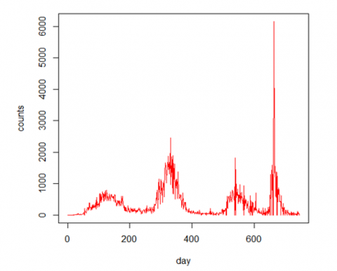
The data used in this study is obtained from. The site contains record of Covid-19 data for many countries, but our interest in this study is the record for Nigeria Covid-19 data. The Data covers 28th February 2020 to 14th March 2022, making a total count of 746. A time plot of the 746 data point on the daily cases of Covid-19 in Nigeria data is presented in Figure 1.
Figure 1. Time series plot of the life data
The descriptive statistics of the life data is presented in Table 3. It should be noted that the summary statistics in Table 3 would be useful in fitting the INGARCH model.
Table 3. Summary statistics of daily new cases of COVID-19 in Nigeria
|
Min. |
Mean |
SD |
Skew. |
Max. |
Var. |
|
0.00 |
341.81 |
44.94 |
4.20 |
6158 |
201546.5 |
Table 3 shows that the data is over-dispersed with higher variance (201546.5) than the mean (341.81).
From Table 3, the Covid-19 data is also positively skewed and over-dispersed just like the simulated data.
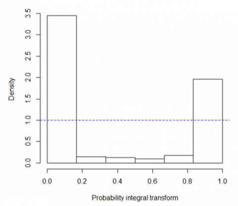
The Non-random Probability Integral Transform (PIT) histogram and Marginal calibration plot new daily cases of COVID-19 positive test in Nigeria for a period of 746 days after first difference is presented in Figure 2.
Figure 2. Non-randomized PIT histogram
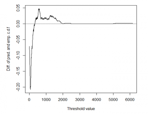
A PIT histogram is used to evaluate the consistency between the observation and the probability forecast. The PIT histogram is a diagnostic tool to assess the goodness-of-fit of probabilistic models. The histogram of a predictive distribution that is centered at the correct value will be uniform, while the occurrence of bin deviation can be thought of as a sign of potential problems with the model's specification, calibration, or fit to the data. If a PIT histogram is flat with no bin with an unusual low or high level, then the predictive distribution is ideal. However, Figure 2 shows the difference between the observations at each value between the highest and lowest observation and the average predictive cumulative distribution function is known as marginal calibration.
Figure 3 shows that the predictive distribution is ideal since the PIT histogram is flat with no bin with an unusual low or high level. The model is well-calibrated showing a curve that closely follows the diagonal line across all levels of predicted probabilities, indicating that the predicted probabilities accurately reflect the actual outcome frequencies across the entire range of predictions. On fitting the models under study to the Covid-19 data, the model selection criteria are presented in Table 4.
Figure 3. Marginal calibration plot
Table 4. Model selection criteria
|
Model |
AIC |
BIC |
QIC |
|
Pois INGARCH |
159564.6 |
159587.7 |
159564.6 |
|
NB INGARCH |
13202.2* |
13229.9* |
475376.7 |
|
ZIP |
280875.6 |
280884.8 |
- |
|
ZINB |
14956.4 |
14568.9 |
- |
|
ARIMA (1,0,1) |
110574.1 |
110686.9 |
- |
The information in Table 4 shows that NB INGRACH model based on model selection criteria outperformed Poisson INGARCH; hence, the NB INGARCH is the most reliable and appropriate for the Covid-19 data.
Results of parameter estimation obtained are presented in Table 5.
Table 5. Parameter estimation
|
|
Estimate |
S.E |
C.I (Lower) |
C.I (Upper) |
|
Intercept |
2.216 |
1.951 |
-1.608 |
6.040 |
|
beta_1 |
0.561 |
0.348 |
-0.122** |
1.243 |
|
alpha_27 |
0.057 |
0.252 |
-0.438 |
0.552 |
|
interv_1 |
0.295 |
0.728 |
-1.132 |
1.722 |
|
interv_2 |
-0.670 |
8.254 |
-16.847 |
15.507 |
|
sigmasq |
67.783 |
- |
- |
- |
From Table 5, the coefficient beta_1 is the regression on the previous observation. It shows that the impact of volatility on the current period was 0.561. If beta is near 1 than 0, it suggests that the volatility is somewhat highly persistent over time. As relating to the new cases of Covid-19 data, the beta is moderately persistent over time, meaning that the number of new cases of Covid-19 will be moderately persistent over time.
The coefficient alpha_27 is the regression values of the conditional mean of the twenty seventh unit back in time. It shows that the impact of the shock was 0.057 in the series. The small shows that the future uncertainty of new cases of Covid-19 will not be so much. The Intervention 1 (interv_1) was t=281 (observation) had 324 counts, while intervention 2 was t=366 (observation) had 341 counts. These are values of t that were close to the mean value of the data (342).
The estimation of the overdispersion coefficient, $\sigma^2$ is 67.783, and $\phi$, the dispersion parameter of Negative Binomial is $1 / \sigma^2$. Following the estimation in Table 5, the fitted model for the new cases of Covid-19 infection in the period $t$ given by $Y_t \mid F_{t-1} \sim {Negbin}\left(\mu_t, 0.015\right)$ is
$\begin{gathered}\mu_t=2.216+0.561 Y_{t-2}+0.057 Y_{t-27} \\ +0.295(t=281)-0.670(t=366)\end{gathered}$ (10)
Relating Table 5 to Eq. (10), the intercept is 2.216, the beta_1 is 0.561, beta_27 is 0.047, interv_1 is 0.295, and interv_2 is -0.670. The scoring function values were estimated and presented in Table 6.
Table 6. Scoring for INGARCH models
|
Score Function |
NB INGARCH (1,1) |
Poisson INGARCH (1,1) |
|
Value |
Value |
|
|
Logarithmic |
6.0470e+00 |
1.795114e+01 |
|
Quadratic |
-8.0477e-03 |
9.756911e-03 |
|
Spherical |
-6.8964e-02 |
-5.001848e-02 |
|
Rankprob |
6.7120e+01 |
5.913281e+01 |
|
Dawseb |
1.0890e+01 |
3.375576e+01 |
|
Normsq |
9.7435e-01 |
2.860757e+01 |
|
Sqerror |
8.9605e+03 |
5.439806e+05 |
The accuracy of the probabilistic predictions was assessed based on scoring function presented in Table 6. The model that gives a lower score function is preferred. INGARCH Binomial outperformed INGARCH Poisson except for “Rankprob”. Table 7 shows the twenty day-ahead predicted cases of Covid-19 data.
Table 7. Predicted cases
|
Day |
Predicted |
CI (Lower) |
CI (Upper) |
|
1 |
10 |
0 |
54 |
|
2 |
69 |
0 |
728 |
|
3 |
47 |
0 |
52 |
|
4 |
119 |
0 |
117 |
|
5 |
80 |
0 |
49 |
|
6 |
168 |
0 |
106 |
|
7 |
136 |
0 |
165 |
|
8 |
163 |
0 |
59 |
|
9 |
186 |
0 |
73 |
|
10 |
160 |
0 |
71 |
|
11 |
219 |
0 |
54 |
|
12 |
190 |
0 |
144 |
|
13 |
231 |
0 |
90 |
|
14 |
200 |
0 |
67 |
|
15 |
236 |
0 |
81 |
|
16 |
203 |
0 |
43 |
|
17 |
240 |
0 |
101 |
|
18 |
181 |
0 |
104 |
|
19 |
214 |
0 |
70 |
|
20 |
201 |
0 |
87 |
The second column of Table 7 shows the predicted cases, the third and fourth column are the 95% upper and lower confidence interval respectively for conditional distribution.
This study focuses on comparing various models for fitting zero-inflated time series count data, using Covid-19 statistics. The study addresses the challenge of modelling time series count data, which often involves over-dispersion and zero-inflation. Various models, including Poisson INGARCH, Negative Binomial INGARCH, Zero-Inflated Poisson, Zero-Inflated Binomial, and ARIMA, are assessed in terms of their suitability and performance. Two critical aspects of analysis are considered: simulation and real-life data.
In the simulation phase, it is observed that Negative Binomial INGARCH models perform exceptionally well, showing superiority over other models such as Poisson INGARCH, Zero-Inflated Poisson, Zero-Inflated Binomial, and ARIMA. This is evident from the AIC and BIC comparisons. In the life data analysis, using Covid-19 statistics, the study indicates that the Zero-Inflated Negative Binomial (ZINB) model demonstrates the best fit based on model selection criteria, particularly AIC and BIC. This result implies that the NB INGARCH model holds substantial promise in effectively modelling over-dispersed and zero-inflated data, which is characteristic of COVID-19 case counts. The results also show that the Covid-19 new cases will be consistent over a period. The implication of the study is that we could adopt a more reliable model for modelling unbounded N-valued integer, such as daily Covid-19 data. Such would help the policy makers to make adequate preparation for health facilities and the required funding. The study aligns with Sustainable Development Goal (SDG) 8 is focused on promoting sustained, inclusive economic growth. The limitation of the study lies in access to data of new Covid-19 cases in other countries for comparative studies.
These results emphasize the significance of choosing an appropriate model that accounts for over-dispersion and zero-inflation, which are common characteristics of count data in various contexts. Adesina et al. [24] showed the superiority of ARFIMA over ARIMA to model Covid-19 data, and future study can investigate the strength of such model against the INGARCH models. The current study offers superior modelling relative to Chan et al. [25] and Busari and Samson [26] who used count regression models, ARIMA, and other machine learning models without giving attention to the count part. Though the study found negative Binomial and ARIMA most appropriate respectively.
The study has demonstrated the superiority of Negative Binomial INGARCH (1,1) model over the competing models and contributes significant insights into the selection of appropriate models for time series count data, with a particular focus on zero-inflated data. The study's findings suggest that Negative Binomial INGARCH model performed well with both simulated and life data.
The study recommends future research to validate these findings with diverse simulation approaches and other real data sources. Additionally, it encourages the exploration of the NB INGARCH model, as it shows potential for being a robust and versatile choice for modelling over-dispersed zero-inflated time series count data, filling a notable gap in existing literature. This research, therefore, contributes valuable insights for both scholars and practitioners dealing with time series count data and offers a promising direction for future studies. Future research can also extend to the INGARCH to mixture models such as Dirichlet mixture models.
[1] Kakad, M., Utley, M., Dahl, F.A. (2023). Using stochastic simulation modelling to study occupancy levels of decentralised admission avoidance units in Norway. Health Systems, 12(3): 317-331. https://doi.org/10.1080/20476965.2023.2174453
[2] Cameron, A.C. (2005). Microeconometrics: Methods and Applications. Cambridge University.
[3] Adesina, O.S., Adekeye, K.S., Adedotun, A.F., Adeboye, N.O., Ogundile, P.O., Odetunmibi, O.A. (2023). On the performance of dirichlet prior mixture of generalized linear mixed models for zero truncated count data. Journal of Statistics Application Probability, 12(3): 1169-1178.
[4] Feng, C. (2020). Zero-inflated models for adjusting varying exposures: A cautionary note on the pitfalls of using offset. Journal of Applied Statistics, 49(1): 1-23. https://doi.org/10.1080/02664763.2020.1796943
[5] Feng, C.X. (2021). A comparison of zero-inflated and hurdle models for modeling zero-inflated count data. Journal of Statistical Distributions and Applications, 8: 8. https://doi.org/10.1186/s40488-021-00121-4
[6] Agarwal, D.K., Gelfand, A.E. Citron-Pousty, S. (2002). Zero-inflated models with application to spatial count data. Environmental and Ecological Statistics, 9: 341-355. https://doi.org/10.1023/A:1020910605990
[7] Adedotun, A.F., Adesina, O.S., Onasanya, O.K., Onos, E.S., Onuche, O.G. (2022). Count models analysis of factors associated with road accidents in Nigeria. International Journal of Safety and Security Engineering, 12(4): 533-542. https://doi.org/10.18280/ijsse.120415
[8] Lu, J., Meyer, S. (2022). A zero-inflated endemic-epidemic model with an application to measles time series in Germany. Biometrical Journal, 65(8): 2100408. https://doi.org/10.1002/bimj.202100408
[9] Shi, Y., Dai, W., Long, W. (2021). A new deep learning-based zero-inflated duration model for financial data irregularly spaced in time. Frontiers in Physics, 9: 651528. https://doi.org/10.3389/fphy.2021.651528
[10] Pittman, B., Buta, E., Krishnan-Sarin, S., O’Malley, S.S., Liss, T., Gueorguieva, R. (2020). Models for analyzing zero-inflated and overdispersed count data: An application to cigarette and marijuana use. Nicotine and Tobacco Research, 22(8), 1390-1398. https://doi.org/10.1093/ntr/nty072
[11] Adesina, O.S., Agunbiade, D.A., Oguntunde, P.E. (2021). Flexible Bayesian Dirichlet mixtures of generalized linear mixed models for count data. Scientific African, 13: e00963. https://doi.org/10.1016/j.sciaf.2021.e00963
[12] Hacker, R.S., Hatemi-J, A. (2022). Model selection in time series analysis: Using information criteria as an alternative to hypothesis testing. Journal of Economic Studies, 49(6), 1055-1075. https://doi.org/10.1108/JES-09-2020-0469
[13] Hasan, F.M., Hussein, T.F., Saleem, H.D., Qasim, O.S. (2024). Enhanced unsupervised feature selection method using crow search algorithm and Calinski-Harabasz. International Journal of Computational Methods and Experimental Measurements, 12(2): 185-190. https://doi.org/10.18280/ijcmem.120208
[14] Oluwadare, J.R., Adesina, O.S., Adedotun, A.F., Odetunmibi, O.A. (2024). Estimation techniques for generalized linear mixed models with binary outcomes: Application in medicine. International Journal of Computational Methods and Experimental Measurements, 12(3): 323-331. https://doi.org/10.18280/ijcmem.120312
[15] Aknouche, A, Almohaimeed, B.S. Dimitrakopoulos, S. (2022). Forecasting transaction counts with integer-valued GARCH models. Studies in Nonlinear Dynamics & Econometrics, 26(4): 529-539. https://doi.org/10.1515/snde-2020-0095
[16] Alwan, E.H., Al-Qurabat, A.K.M. (2024). Optimizing program efficiency by predicting loop unroll factors using ensemble learning. International Journal of Computational Methods and Experimental Measurements, 12(3): 281-287. https://doi.org/10.18280/ijcmem.120308
[17] Zhang, C., Han, J. (2021). Data Mining and Knowledge Discovery. In Urban Informatics, Springer, Singapore. https://doi.org/10.1007/978-981-15-8983-6_42
[18] Liu, M., Zhu, F., Li, J., Sun, C. (2023). A systematic review of INGARCH models for integer-valued time series. Entropy, 25(6): 922. https://doi.org/10.3390/e25060922
[19] Liboschik, T., Fokianos, K., Fried, R. (2017). Tscount: An R package for analysis of count time series following generalized linear models. Journal of Statistical Software, 82(5): 1-51. https://doi.org/10.18637/jss.v082.i05
[20] Christou, V., Fokianos, K. (2014). Quasi-likelihood inference for negative binomial time series models. Journal of Time Series Analysis, 35(1): 55-78. https://doi.org/10.1111/jtsa.12050
[21] R Core Team. (2013). R: A language and environment for statistical computing. Foundation for Statistical Computing, Vienna, Austria. https://www.gbif.org/tool/81287/r-a-language-and-environment-for-statistical-computing.
[22] Liboschik, T., Fried, R., Fokianos, K., Probst, P. (2020). tscount: Analysis of count time series. https://cran.r-project.org/web/packages/tscount/index.html.
[23] Malki, Z., Atlam, E.S., Ewis, A., Dagnew, G., Alzighaibi, A.R., ELmarhomy, G., Elhosseini, M.A., Hassanien, A.E., Gad, I. (2021). ARIMA models for predicting the end of COVID-19 pandemic and the risk of second rebound. Neural Computing and Applications, 33: 2929-2948. https://doi.org/10.1007/s00521-020-05434-0
[24] Adesina, O.S., Onanaye, S.A., Okewole, D., Egere, A.C. (2020). Forecasting of new cases of Covid-19 in Nigeria using autoregressive fractionally integrated moving average models. Asian Research Journal of Mathematics, 16(9): 135-146. https://doi.org/10.9734/arjom/2020/v16i930226
[25] Chan, S., Chu, J., Zhang, Y., Nadarajah, S. (2021). Count regression models for COVID-19. Physica A: Statistical Mechanics and its Applications, 563: 125460. https://doi.org/10.1016/j.physa.2020.125460
[26] Busari, S.I., Samson, T.K. (2022). Modelling and forecasting new cases of Covid-19 in Nigeria: Comparison of regression, ARIMA and machine learning models. Scientific African, 18: e01404. https://doi.org/10.1016/j.sciaf.2022.e01404