Yousra Kateb*![]() | Abdelmalek Khebli
| Abdelmalek Khebli![]() | Hocine Meglouli
| Hocine Meglouli![]()
© 2024 The authors. This article is published by IIETA and is licensed under the CC BY 4.0 license (http://creativecommons.org/licenses/by/4.0/).
OPEN ACCESS
Rolled steel is a major product of ferrous metalworking. It is a popular metal structure construction technology. Though a big amount of the finished product may be flawed, the process of manufacturing must be improved. It is critical to correctly classify hot-rolled strip faults. As a result, in recent years, numerous machine-learning-based automated visual inspection (AVI) systems have been created. However, these approaches lack several critical components, such as insufficient RAM, which causes complexity and slowness during implementation. Long execution durations, in general, cause the process to be delayed or completed later than expected. A shortage of faulty samples is also a significant difficulty in steel defect detection, as the imbalance between the huge number of non-defective photos and the defective ones causes the algorithm to be unfair in categorization. To address these three issues, a deep CNN model is created in this study. The backbone architecture is a pre-trained NasNet-Mobile that has been fine-tuned with particular parameters to be compatible with the required data. Despite having 27 times less data than other articles' datasets, the model detects steel surface photos with six defects with 99.51% accuracy, exceeding earlier methodologies. This study is useful for surface fault classification when the sample size is small, the software is not quite as effective, or time is limited. Avoiding these issues will help the steel industry improve safety and end product quality while also saving time and money.
few samples, image classification, NasNet-mobile, pre-trained CNN, steel surface inspection
Hot-rolled strip steel is widely utilized in automobile manufacture, aircraft, and light industries as one of the steel industry's key products [1, 2]. One of the most important indications of strip steel's market competitiveness is surface quality. Because of the raw material's influence, the strip steel surface will unavoidably change due to the materials, rolling method, and external environment. In the manufacturing process, oxide scale, inclusions, scratches, and other imperfections emerge that are not visible. It not only has a negative effect on appearances, but it also decreases fatigue resistance. However, these faults cannot be completely avoided by improving the technique over time [3]. Therefore, the surface fault categorization may be utilized as a reference throughout the production operation. The objective of increasing yield and minimizing manufacturing costs is achieved through suitable adjustment. A lot of issues arise during the real-time examination of steel surfaces. Some of these issues include the following:
Hazardous location: Putting inspection equipment (illumination system, camera, and certain signal processing equipment) in hot rolling mills is extremely dangerous. The presence of dust, grease, grime, water droplets, and vapor is common. Furthermore, the lighting system and cameras must be protected from stress and vibration. On a daily, monthly, and annual basis, heavy equipment is moved in and out of the site. The aforementioned concerns necessitate the adoption of appropriate physical and environmental safeguards for site equipment.
Operation speed: The high working speed of surface inspection equipment is generally 20 m/s for flat steel goods and 100 m/h for long products, necessitating the use of sophisticated image processing equipment and software with a short execution time.
Surface defect types: Surface flaws in steel merchandise are quite diverse, with nine primary classes and 29 subclasses. These flaws are not governed by norms, and their features and categorization differ between factories and operators, as well as their appearance, which might alter according to variances in the manufacturing process.
HRC (hot roll coil) is the most common finished steel form in the world and an important raw material for manufacturers. It is a vital substance that necessitates precise and quick spot pricing and analysis. Many factors, ranging from raw material costs to global trade agreements, eventually influence the pricing of the carbon steel products customers purchase. The three main factors are described:
Firstly, steel starts with iron ore, scrap, coking coal, and natural gas. These resources' prices are influenced by the producing countries and traded on exchanges such as CME (Chicago Mercantile Exchange). Secondly, the macro-economic factors influencing supply and demand dynamics have a significant effect. For example, when the US administration imposed a 25% tax on steel in early 2018, the price of HRC increased in the United States. Thirdly, depending on the end-use of a product, HRC is subjected to a variety of mill treatments, many of which add value but come at an additional expense.
Steel surface inspection currently falls into two categories: conventional techniques and deep learning techniques. In the traditional category, features are extracted using Support Vector Machine (SVM) [4], Random Forest [5], k-nearest neighbor (KNN) [6], and many different other classifiers. However, because there are no obvious guidelines for the distribution of flaws on the steel images, extracting the features is challenging, resulting in difficulties utilizing the detection algorithm as well as poor recognition accuracy. The deep learning approaches are mainly based on convolutional neural networks; these CNNs are used to classify defective surfaces on steel products [7]. Here, features are extracted directly from the image, which results in high accuracy, high speed, and more adaptability [8].
As a consequence, improving surface defect classification accuracy in hot-rolled strips in order to minimize the frequency of human intervention in defect classification may result in considerable economic and social benefits. On the one hand, quality inspectors may avoid working late at night, which is good for their health. On the other hand, mistakes caused by fatigue and other variables of quality inspectors will be significantly minimized, boosting the performance and productivity of the strip steel and offering higher advantages to the steel factory. In brief, the paper's contributions are as follows:
Significance of the research:
The key objective of this study is to assist small industries in pursuing the defect detection process using such little software and a few samples of defected images in a shorter time. This will lead to the good development of small mills and fewer potential operators. This research would be carried out with more improvement according to the client’s needs.
Experts tended to identify problems manually, which was imprecise and error-prone [9]. Furthermore, as a result of the identical flaws, various expert judgments will be formed, leading to incorrect types and classes of strip steel flaws, diminishing defect detection reliability. Recognition results based on researchers' subjective judgments are generally inadequate [10, 11].
To overcome the limitations of manual identification, researchers have addressed a number of solutions based on machine learning technology.
Meta-learning-based method. It trains a meta model to acquire the knowledge of multiple tasks, such as the Model-Agnostic Meta-Learning algorithm (MAML) proposed by Finn et al. [12] and the Long Short Term Memory network (LSTM) developed by Ravi and Larochelle [13]. Existing meta-learning algorithms often use an LSTM or Recurrent Neural Network (RNN) structure within the model, however these algorithms have significant temporal complexity and sluggish running speed. As a result, it is inappropriate for industrial use.
The Grayscale Covariance Matrix (GLCM) as well as the Discrete Shear Transform were used to suggest a classification approach [14]. (DST). After obtaining multi-directional shear characteristics from the pictures, a GLCM calculation is done. It then performs an important aspect analysis involving high-dimensional feature vectors before being passed into a support vector machine (SVM) to identify surface faults in strip steel. The fundamental disadvantage of the GLCM technique is its large matrix dimensionality, which necessitates the use of highly capable software.
In the study [15], The authors presented a unique multi-hyper-sphere SVM with extra information (MHSVM+) approach for revealing hidden information in defective data sets using an additive learning model. It has a higher classification accuracy on defect datasets, particularly damaged datasets. However, SVM algorithm underperforms in large data sets with noise and overlapping target classes, and underperforms when features exceed training data samples.
The authors [16] designed a one-class classification technique made up of generative adversarial networks (GAN) [17] and SVM. It trains an SVM classifier with GAN-generated features. It further enhances the loss function, thereby improving the stability of the model. Regrettably, the aforementioned standard Machine Learning techniques often need substantial feature engineering, which greatly raises costs [18].
Traditional machine learning-based algorithms, as previously indicated, are frequently impacted by defect size and noise. Furthermore, this method's accuracy is insufficient to fulfill the practical criteria of automated defect identification. Some elements must be created by hand, as well as the scope of the application is highly limited.
Deep learning-based techniques, notably convolutional neural networks (CNN), have experienced great success in image classification tasks in recent years [19, 20]. CNN has great characterization capabilities [21, 22] and is very successful at recognizing strip surface flaws [6, 8, 17].
Authors [23] built on GoogLeNet [24] and improved it slightly by including identity mapping. To minimize overfitting, the dataset was augmented using the data augmentation approach.
SqueezeNet [25] was applied in the study [26] to present an end-to-end effective model. The multiple receptive field scheduling, which may provide scale-related high-level features, was added to SqueezeNet. It is beneficial to low-level feature training and it can classify strip steel surface faults fast and consistently. One of SqueezeNet's key disadvantages is its low accuracy when compared with larger and more complicated models.
Authors [27] proposed a modified AlexNet [28] and SVM-based intelligent surface defect inspection system for hot-rolled steel strip pictures. Due to receptive field limitations, CNN-based classification models have excellent fitting ability but poor global representation ability. Obtaining a significant number of fault samples in complicated industrial situations is difficult, therefore increasing the dataset has become a pressing issue that must be addressed. The attention mechanism, on the contrary, has been shown to enable the model to focus on more significant information, resulting in higher recognition accuracy. In contemporary research, however, attention mechanisms are rarely used to define strip steel surface defects [29].
Traditional Machine Learning methods often require considerable feature engineering, which raises the cost significantly.
Our strategy consists of four main stages:
Step 1: we preprocess the data and organize it into six types of defects (patches, crazing, pitted surface, scratches, rolled in scale, inclusion). This dataset is available on the NEU Steel detection competition website [30].
Step 2: we use the pre-trained CNN called NasNet-Mobile as the backbone of the model with which we extract the image features; the top layers will be frozen to use the ImageNet saved weights. The last block is then fully erased and replaced with an entirely new one (global average pooling, dropout, exponential linear unit (ELU) to represent the dense layers, as well as a Softmax function for the prediction and classification layer).
Step 3: we fine-tune the model with the obtained weights and switch between optimizers (ADAM optimizer, ADAMAX optimizer) to get the best results.
Step 4: we make the comparison to pick up the best fine-tuned model (we take into consideration the three metrics: Accuracy vs. Executing time vs. Model lightness).
3.1 Steel surface defect dataset
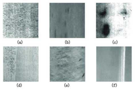
The NEU surface defect database includes six types of hot-rolled steel strip surface flaws: rolled-in scale (RS), inclusion (In), patches (Pa), crazing (Cr), pitted surface and (PS) and scratches (Sc) [30]. The database contains 1800 photos (300 for each surface fault type). Figure 1 depicts sample photos of various common faults. The dataset collection was chosen because it contains fewer photos than other databases, allowing us to compare the performance of our technique with this little quantity of data to other papers' datasets (Table 1).
A part of 80% of the data was randomly selected (there are 240 photos for each fault type.) in the NEU dataset to form the training data. The other rest (20%) is used to validate the classification of the network. All data was augmented using “Image-Data-Generator” in Tensorflow [31] and Keras [32] libraries. Rotation (0°, 45°, 90°, 180°), horizontal flipping, shearing (0.2) and zooming (0.2). Each image's pixel values were adjusted to fall within the range of [-1; 1] before being fed into our network.
Table 1. Summary of number of data in previous works
|
Proposed Algorithm |
Image Modality |
Number of Images |
|
Deep residual neural network [22] |
Severstal: Steel Defect Detection |
87704 |
|
DenseNet, ResNet,U- Net [33] |
Severstal: Steel Defect Detection |
12568 |
|
ResNet-50, ResNet-152 [34] |
Severstal: Steel Defect Detection, NEU steel database |
9385 |
|
Our model: NASNet-Mobile |
NEU: Steel Defect Dataset |
1800 |
Figure 1. Several metallic surface fault samples. (a) Crazing. (b) Inclusion. (c) Patches. (d) Pitted surface. (e) Rolled in scale. (f) Scratches [35]
3.2 Classification model—Improved NASNet-Mobile
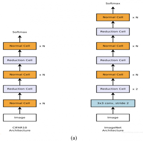
The technique of automating the construction of neural network topology in order to get the best outcomes on a certain job is known as Neural Architecture Search (NAS). The task is to develop the architecture with few resources and as little human help as possible. Authors [36] created the NasNet architecture, a neural architecture search network that trains to obtain the most correct parameters from produced architecture using a recurrent neural network (RNN) and reinforcement learning. Designing a CNN architecture requires a long time when the material is large, for instance the ImageNet dataset. They subsequently developed an CNN framework capable of searching for the best architecture in a small set of data and then transferring the best architecture to be trained on huge datasets; this architecture is known as "learning transferable architectures". The NASNet-Mobile architecture may be scaled based on data volume.
• Identity
• 1 × 7 then 7 × 1 convolution
• 3 × 3 average pooling
• 5 × 5 max pooling
• 1 × 1 convolution
• 3 × 3 depthwise-separable convolution
• 7 × 7 depthwise-separable convolution
• 1 × 3 then 3 × 1 convolution
Figure 2. (a) CIFAR10 dataset (left) and ImageNet (right) dataset architectures (b)Normal cell (left) and reduction cell (right) [36]
• 3 × 3 dilated convolution
• 3 × 3 max pooling
• 7 × 7 max pooling
• 3 × 3 convolution
• 5 × 5 depthwise-separable convolutions [36]
3.2.1 Depthwise and pointwise convolutions
The NasNet-Mobile framework is based on depthwise separable convolutions [37], a sort of factorized convolution in which a conventional convolution is divided into a depthwise convolution and also a 1 x 1 convolution known as a pointwise convolution. NasNet-Mobile use depthwise convolution in order to apply an individual filter for each input channel. The pointwise convolution then combines the depthwise convolution outputs with a 1 x 1 convolution. A conventional convolution filters and mixes inputs in a single step to generate a new set of outputs. This is divided into two layers by the depthwise separable convolution, one for filtering and another for combining. This factorization significantly reduces processing and model size. Depthwise separable convolutions are made up of two layers, which are depthwise and pointwise. We use depthwise convolutions (input depth) to set up a single filter for each input channel. The depthwise layer output is then linearly mixed using pointwise convolution, which is a basic 1 x 1 convolution (Eq. (1)).
$G_{k, l, m}=\sum_{i, j} \hat{k}_{i, j} * F_{k+i-1, i+j-1, m}$ (1)
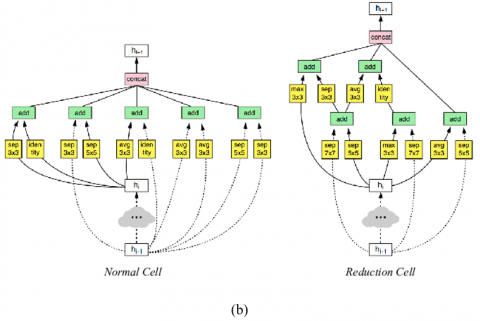
$\mathrm{K}$ is the depthwise convolutional kernel with a size of $\mathrm{D}_{\mathrm{k}} \mathrm{X}$ $\mathrm{D}_{\mathrm{k}} \times \mathrm{M}$ Where the $\mathrm{m}^{\text {th }}$ filter in $K^{\wedge}$ is applied to the $\mathrm{m}^{\text {th }}$ channel in $\mathrm{F}$ to output the $\mathrm{m}^{\text {th }}$ channel of the filtered output feature map G. As shown in Figure 2(a) and Figure 2(b), RNN merges two hidden layers to move on to the following hidden layer.
Figure 3. Convolution cell block acquired via RNN exploration
We study modifications in architectural configuration of each reference structure empirically (Section II). We use transfer learning from network models trained on ImageNet [38] in the simplified CNN framework by removing the block and replacing it with a new block containing global average pooling, dropout, dense, as well as a Softmax function for the last prediction layer to forecast the steel defect class (Figure 3). For the first part of training (before fine-tuning), the whole architecture is frozen except for the final created block. Following that, we unfreeze the model's top so that it may train again to the desired goal (steel fault classification). This avoids the network from over-fitting throughout training and allows its model to learn quicker and for a longer period of time, resulting in improved generalization. Using the light-weight NasNet architecture provides various advantages, including improved model training, being less prone to short dataset over-fitting, and being deployable in other embedded systems.
3.2.2 NASNet-Mobile-based defect classification
There are three main reasons of taking this CNN as the backbone of our model. Firstly, its lightness as it takes only 23 MB in the memory which is too smaller in comparison with other models (VGG16 takes 549 MB, ResNet52 takes 232 MB, NASNet-Large takes 343 MB…etc.). Secondly, the number of parameters, this model is built with only 5.3 million parameters which is comparatively very small (for example the VGG16 is built with 143.7 million parameters, it is then 27 times larger than our NASNet-Mobile model). The last reason is that this model takes only 27 ms per inference step in a CPU and 6.7 ms per inference step in a GPU, it is then 60 times less than the EfficientNetB7 (with 1578.9 ms per inference step).
Figure 4. General structure of the proposed approach
NasNet-Mobile's basic model is pre-trained with 1,056 output channels for ImageNet [38] recognition. This architecture's core experimentation is around the amount of regular cells in the model. We employed three reduction cells with three regular cells in our modified NASNet-Mobile design (Figure 4). The total number of parameters is 4,376,022, of which only 106,306 (2.42% are trainable) and the rest are frozen.
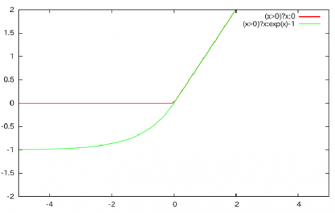
We use the pre-trained NASNet-Mobile framework as the backbone building design, which consist six cells (reduced and normal), followed by a newly constructed defect classification block that includes a convolution layer, dropout, dense, and global average pooling. The activation function is "ELU" rather than "ReLU" in the first dense layer. ELU, or Exponential Linear Unit, is a function that converges cost to zero faster and produces more accurate results [39]. In contrast to other activation functions, ELU contains an extra alpha constant that needs to be positive, as seen in Eq. (2).
$R(z)= \begin{cases}z & \text { when } z>0 \\ \alpha \cdot(\exp (z)-1) & \text { when } z<0\end{cases}$ (2)
ELU is extremely similar to RELU, with the exception of the negative inputs. They are both in identity function form for non-negative inputs. ELU, on the other hand, smoothies progressively until their output equals $-\alpha$, whereas RELU smoothies substantially (Figure 5). The reason for using ELU instead of ReLU as an activation function is because ELU smoothes out gradually till it reaches $\alpha$, whereas RELU smoothes out dramatically. Furthermore, unlike ReLU, ELU can provide negative outputs.
The ELU is a continuous and differentiable activation function that offers faster training times compared to other linear non-saturating functions like ReLU with its other different versions (Leaky-ReLU (LReLU) and Parameterized-ReLU (PReLU).). It doesn't suffer from dying neurons, exploding or vanishing gradients. As compared to other activation functions like ReLU, Sigmoid, and Hyperbolic Tangent, it achieves more accuracy.
Steel surface defect classifier variables can be updated by reducing a multi-class loss function known as Categorical crossentropy (Eq. (3)).
LOSS $=-\sum_{i=1}^{\text {output size }} y_i * \log \hat{y}_i$ (3)
where, yi represents the i-th scalar value in the model output, yi indicates the equivalent goal value, and output size refers to the number of scalar values in the output of the model.
Figure 5. Graph showing the difference between ELU (green) and ReLU (red) activation functions [39]
Following the development of the basic NasNet-Mobile model for steel surface defect inspection, we propose many viable strategies for improving accuracy and reducing execution time. First, data augmentation is used to get more features to be learnt by the model. Second, a new block, which we already defined, is added at the bottom of the model for the prediction part, this block will help improve accuracy and reduce model parameters and executing time. Third, we switch between optimizers to find the best one (ADAM and ADAMAX). Finally, the learning rate is reduced using the exponential decay as in Eq. (4) then we apply the early stopping when the model accuracy cannot improve anymore. The model restores the best weights.
$y=a(1-b)^x$ (4)
where, y represents the final value, a represents the initial value, b represents the decay factor, in addition x is the value of time that has elapsed.
4.1 Model implementation
Our method is deployed under the publicly available Python framework from Google Colaboratory [40]. Tesnorflow [31], Keras, Matplotlib, NumPy, and Glob are the main libraries used in this implementation. We took 80% of the photos in the NEU (NEU) collection as training data (240 images for every single fault category) and 20% as validation data. Before as well as after fine-tuning the network, performance is evaluated. Table 2 shows the values of the hyperparameters used to train this CNN.
The experiments were performed with Windows 10 Professional on the Intel® Core (TM) i5 7200U, 64-bit platform with 8GB of RAM and NVIDIA RTX 2070, as we took advantage of the free available GPU on the Google Colab Platform. The training with the surface defect dataset was so fast. It took only 3414 seconds (56 minutes and 54 seconds) to train the model before fine-tuning and 528 seconds after fine-tuning (8 minutes and 48 seconds).
Table 2. Hyperparameters used to train the NasNet-Mobile convolutional neural network
|
Hyperparameters |
Before Fine-Tuning |
After Fine-Tuning |
|
Number of epochs |
20 |
100 |
|
Steps per epoch |
6 |
6 |
|
Number of trainable parameters |
106,306 |
4,376,022 |
|
Learning rate mode |
Max |
Exponential decay |
|
Restore best weights |
True |
True |
|
Learning rate value |
Min = 1 e-8 Max = 0.01 Patience = 3 Factor = 25% |
Min = 0.01 Max = 0.1 Steps = 20 Factor 50% |
|
Early stopping |
Patience = 10 Min delta = 0.005 |
Patience = 10 |
|
Loss |
Categorical crossentropy |
Categorical crossentropy |
|
Optimizer |
ADAM |
ADAMAX |
Table 3. Performance metrics of NasNet-Mobile in the training and validation dataset before fine-tuning
|
Metrics |
Training Dataset |
Validation Dataset |
|
Accuracy |
99.51% |
97.78% |
|
Loss |
0.028 |
0.064 |
|
Precision |
99.51% |
98.60% |
|
Recall |
99.51% |
97.78% |
|
Area under the curve AUC |
100% |
99.96% |
4.2 Model evaluation
Our model was running twice, once without fine-tuning the parameters and again with fine-tuning the parameters. The following deep learning metrics are used to assess the model: accuracy, loss, recall, AUC, FP, FN, TP, TN, and precision. With different datasets for training and validation, we compare these measures before and after fine-tuning.
The results are shown in the following tables and graphs, along with an analysis of each one.
The metrics in Table 3 show very promising results in both the training and validation datasets. We can note a slight decrease between them, and this is because the model learns from the training data, which makes it more reliable, but according to the validation data, we know that it has only 20% of the total data, and the model has never learned from it. Since evaluating the model on the training dataset might produce in biased results, it is tested using a held-out sampling to offer an impartial evaluation of its competence. Strategies that may be utilized to mitigate the difference in performance include model fine-tuning and dataset augmentation to ensure the model can learn additional features.
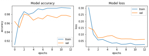
Figure 6. Accuracy and loss curves before fine-tuning the NasNet-Mobile
Figure 6 displays the training as well as validation curves of the optimization for NasNet-Mobile developed with the previously stated dataset of 1800 photos enhanced through Image Data Generator (These findings were achieved before to fine tuning). The training spanned 20 epochs, including a break at the 12th. We can notice a declining trend as the number of epochs grows, which is followed by validation loss and training loss (Figure 7). During the learning phase, the model appears to identify the visual prominence of the reference picture and the candidate image. As a result, the loss attained during training tends to decrease. The images were chosen at random during the testing phase. These images are from a different class that has never been shown to the network during training. Consequentially, we observe that as the training steps progress, the accuracy of the set to be tested follows that of the set used for training while remaining only slightly inferior. This shows that the algorithm, which was trained on cases of the training set, predicts the cases that weren't in the training set correctly.
Figure 7. Precision and accuracy curves before fine-tuning the NasNet-Mobile
Precision is the proportion of properly classified examples (5), while recall (also known as sensitivity) is the proportion of recovered relevant instances (6). Relevance thus determines precision and recall.
Precision $=\frac{\mathrm{TP}}{\mathrm{TP}+\mathrm{FP}}$ (5)
Recall $=\frac{\mathrm{TP}}{\mathrm{TP}+\mathrm{FN}}$ (6)
Accuracy $=\frac{\mathrm{TP}+\mathrm{TN}}{\mathrm{TP}+\mathrm{TN}+\mathrm{FP}+\mathrm{FN}}$ (7)
As we can see in the previous curves (Figure 8) and in (Table 3), the best-achieved precision is about 99.51% in the training and 98.6% for the validation. The recall is about 99.51% for training and 97.78% for validation dataset. These results were obtained before the fine-tuning.
Table 4. Performance metrics of NasNet-Mobile in the training and validation dataset after fine-tuning
|
Metrics |
Training Dataset |
Validation Dataset |
|
Accuracy Loss |
100% 0.0245 |
98.06% 0.0729 |
|
Precision |
100% |
98.04% |
|
Recall |
100% |
97.50% |
|
Area under the curve AUC |
100% |
99.44% |
Figure 8. Training with validation loss
Figure 9. Accuracy (left) and loss (right) curves for fine-tuned NasNet-Mobile CNN
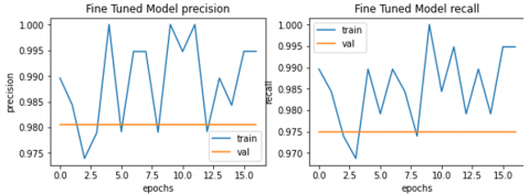
Figure 10. Precision and recall loss in the fine-tuned model
The training process was early stopped, as shown in Figure 9, because there was no improvement during three consecutive epochs. We can clearly see the instability of both accuracy and loss in the training and validation datasets, as shown in Table 4, even though the accuracy of the model can reach 100%, which is very good compared with such a small amount of data (only 300 images per class, whereas 240 for training and 60 for validation). This instability is caused by the absence of batch normalization in the experiments (Figures 9 and 10). Batch normalization enhances the training process by reducing internal covariate shifts, improving stability, and optimizing the model. It also improves generalization by normalizing layer activations, reducing overfitting, and reducing initial weight sensitivity. Batch normalization also allows for higher learning rates, accelerating the training phase as well as minimizing the need for precise initialization (no batch normalization layer was included in our architecture in the first experiment). To overcome this issue, we should address model fine-tuning, like adding different batch normalization layers and training the model again.
4.3 Comparative study
In this part, we will compare our model to prominent steel surface inspection methodologies already in use. We take into consideration not only the accuracy but also the terms of execution time, model lightness (number of parameters), and data size.
Table 5. The classification accuracy (%) for several state-of-the-art steel surface fault classifiers taking into account the triplet model lightness vs. running time vs. data size
|
Method |
Accuracy |
Model Lightness (nbr of prmtrs) |
Time (ms) Per Inference step |
Data Size |
|
[34] |
96.91% |
25.6 million |
58.2 |
87704 |
|
[33] |
98.56% |
25.6 million |
77.1 |
12568 |
|
[41] |
97.27% |
60 million |
10.3 |
26334 |
|
Our method (Developed NasNet-Mobile) |
99.51% |
5.3 million |
27.0 |
1800 |
Table 6. The evaluation of classification error depending on various activation functions, the model uses the name of the activation function wrapped in parenthesis
|
Method |
Error Rate (%) |
|
CNNs (Sigmoid) |
12.8721 |
|
CNNs (Hyperbolic Tangent) |
18.1129 |
|
CNNs (ReLUs) Recall |
9.5018 |
|
CNN (LUs) |
0.6292 |
|
Our method (ELUs) |
0.028 |
According to Table 5, we can obviously say that our model beats the aforementioned models regard to accuracy, while it achieves a 99.51%, which is higher in comparison with other accuracies. The proposed NasNet-Mobile can reach very satisfying results with lower model parameters and running time, as well as it doesn’t require large data: 48 times lower than the model [34], 7 times lower than the model [33] and 14 times lower than the model [41]. Our model seems to be the lighter (only 5.3 million parameters which is so low compared to DeCAF model [41] with 60 million parameters and 25.6 million parameters of residual neural network [22].
Finally, the running time of our network is faster than the other's executing time. As we can see, it is three times less than the model [33] and 2.5 times less than the model [22]. The error rate of our model is the lowest compared to other models error rates. In Table 6, the error rate of our model is 0.028, which is 22 times less than the CNN method with LU’s activation function. This means that our model can learn better with fewer errors and better accuracy.
In this paper, we have suggested a novel method based on the pre-trained NASNet-Mobile CNN to classify defects in steel sheets. Here are the main findings of the research:
The issue of accurate classification when the memory is insufficient is set using the NASNet-Mobile network, which has a small number of parameters compared to other CNNs (5.3 million parameters). The top layers of this CNN were frozen, which helped to use less memory and calculations without losing weight. The long executing time dilemma is fixed using the free GPU available on the Google Colab Platform. The problem of dataset scarcity is addressed in this paper and solved due to the potency of this CNN, which can get the necessary features of the image due to its long depth (389 layers), which can extract more features even though the dataset number is tiny.
The modification of hyper-parameters gave an improvement to the model when fine-tuned. We found out that the ADAMAX optimizer is better than the ADAM optimizer in this modified NasNet-Mobile architecture. Thus, we could note a slight improvement in both accuracy and error rate. The Adam optimizer adjusts weights in inverse proportion to the scaled L2 norm of previous gradients, whereas AdaMax expands this to the infinite norm of previous gradients.
The model has been justified, and the last block was entirely removed and outright replaced with a new block. Hence, other modifications were adopted to match the requirements of steel image features. An ELU activation function was set in the convolution layers. We meant to use this activation function, and this is to exploit its advantages. This activation function helps solve the dying RELU problem where the gradient value is 0 on the graph's negative side. As a consequence, the weights and biases of certain neurons are not updated throughout the backpropagation process. This can result in dead neurons that are never triggered. By inserting a log curve for negative input values, ELU can address the RELU dying problem. It then assists the network in adjusting weights and biases in the proper direction. The ELU activation function can increase model performance and network robustness. It likewise gradually smoothies until its output equals zero, whereas RELU dramatically smoothes.
A dropout (0.2) was added after each fully connected layer, and a global average pooling was placed before the dense layer, which helped minimize time and memory during the model implementation. Learning rate scheduling enables us to make use of larger steps for the first couple epochs, then gradually lower the number of steps as the weights approach their ideal value.
More improvements can be achieved by gathering more training data and/or strengthening the network's architecture and fine-tuning its hyper-parameters instead of raising the training epochs under the present structure, which might result in overtraining.
In general, we can conclude that the suggested algorithm can be adopted in image processing tasks such as classification tasks to overcome the main three challenges : time consumption, memory insufficiency, and limited data confronts in small mills and non-powerful operators.
This work is supported by the GOOGLE Colaboratory, free provided GPU, PYTHON community as well as open access GITHUB and Kaggle databases.
|
AI |
Artificial Intelligence |
|
CNN |
Convolutional neural network |
|
DNN |
Deep neural network |
|
TP |
True positive |
|
TN |
True negative |
|
FP |
False positive |
|
FN |
False negative |
|
CPU |
Central Processing Unit |
|
GPU |
Graphic Processing Unit |
[1] Yi, L., Li, G., Jiang, M. (2017). An end-to-end steel strip surface defects recognition system based on convolutional neural networks. Steel Research International, 88(2): 1600068. https://doi.org/10.1002/srin.201600068
[2] Kateb, Y., Meglouli, H., Khebli, A. (2020). Steel surface defect detection using convolutional neural network. Algerian Journal of Signals and Systems, 5(4): 203-208. https://doi.org/10.51485/ajss.v5i4.122
[3] Neogi, N., Mohanta, D.K., Dutta, P.K. (2014). Review of vision-based steel surface inspection systems. EURASIP Journal on Image and Video Processing, 2014(1): 1-19. https://doi.org/10.1186/1687-5281-2014-50
[4] Zhang, M., Zheng, H.F., Hao, N.I. (2019). Ultrasonic image defect classification based on support vector machine optimized by genetic algorithm. Acta Metrologica Sinica, 40: 887-892.
[5] Du, P., Samat, A., Waske, B., Liu, S., Li, Z. (2015). Random forest and rotation forest for fully polarized SAR image classification using polarimetric and spatial features. ISPRS Journal of Photogrammetry and Remote Sensing, 105: 38-53. https://doi.org/10.1016/j.isprsjprs.2015.03.002
[6] Kim, C., Choi, S., Kim, G., Joo, W. (2006). Classification of surface defect on steel strip by KNN classifier. Journal of the Korean Society for Precision Engineering, 23(8): 80-88.
[7] Wang, J., Luo, L., Ye, W., Zhu, S. (2020). A defect-detection method of split pins in the catenary fastening devices of high-speed railway based on deep learning. IEEE Transactions on Instrumentation and Measurement, 69(12): 9517-9525. https://doi.org/10.1109/TIM.2020.3006324
[8] Li, Z., Tian, X., Liu, X., Liu, Y., Shi, X. (2022). A two-stage industrial defect detection framework based on improved-YOLOv5 and optimized-inception-resnetv2 models. Applied Sciences, 12(2): 834. https://doi.org/10.3390/app12020834
[9] Vannocci, M., Ritacco, A., Castellano, A., Galli, F., Vannucci, M., Iannino, V., Colla, V. (2019). Flatness defect detection and classification in hot rolled steel strips using convolutional neural networks. In: Rojas, I., Joya, G., Catala, A. (eds) Advances in Computational Intelligence. IWANN 2019. Lecture Notes in Computer Science(), vol 11507. Springer, Cham. https://doi.org/10.1007/978-3-030-20518-8_19
[10] Wu, C., Ju, B., Wu, Y., Lin, X., Xiong, N., Xu, G., Li, H., Liang, X. (2019). UAV autonomous target search based on deep reinforcement learning in complex disaster scene. IEEE Access, 7: 117227-117245. https://doi.org/10.1109/ACCESS.2019.2933002
[11] Luo, Q., He, Y. (2016). A cost-effective and automatic surface defect inspection system for hot-rolled flat steel. Robotics and Computer-Integrated Manufacturing, 38: 16-30. https://doi.org/10.1016/j.rcim.2015.09.008
[12] Finn, C., Abbeel, P., Levine, S. (2017). Model-agnostic meta-learning for fast adaptation of deep networks. In International Conference on Machine Learning, pp. 1126-1135.
[13] Ravi, S., Larochelle, H. (2016). Optimization as a model for few-shot learning. In International conference on learning representations. International Conference on Learning Representations.
[14] Ashour, M.W., Khalid, F., Abdul Halin, A., Abdullah, L.N., Darwish, S.H. (2019). Surface defects classification of hot-rolled steel strips using multi-directional shearlet features. Arabian Journal for Science and Engineering, 44: 2925-2932. https://doi.org/10.1007/s13369-018-3329-5
[15] Gong, R., Wu, C., Chu, M. (2018). Steel surface defect classification using multiple hyper-spheres support vector machine with additional information. Chemometrics and Intelligent Laboratory Systems, 172: 109-117. https://doi.org/10.1016/j.chemolab.2017.11.018
[16] Liu, K., Li, A., Wen, X., Chen, H., Yang, P. (2019). Steel surface defect detection using GAN and one-class classifier. 2019 25th International Conference on Automation and Computing (ICAC), Lancaster, UK, pp. 1-6. https://doi.org/10.23919/IConAC.2019.8895110
[17] Goodfellow, I., Pouget-Abadie, J., Mirza, M., Xu, B., Warde-Farley, D., Ozair, S., Courville, A., Bengio, Y. (2020). Generative adversarial networks. Communications of the ACM, 63(11): 139-144. https://doi.org/10.1145/3422622
[18] Li, S., Wu, C., Xiong, N. (2022). Hybrid architecture based on CNN and transformer for strip steel surface defect classification. Electronics, 11(8): 1200. https://doi.org/10.3390/electronics11081200
[19] Krapac, J., Meglouli, H. (2021). Représentations d'images pour la recherche et la classification d'images. Doctoral dissertation, Automatique Appliquée et Traitement du Signal, Université M'hamed Bougara - Boumerdes Algeria.
[20] Kateb, Y., Meglouli, H., Khebli, A. (2023). Coronavirus diagnosis based on chest X-ray images and pre-trained DenseNet-121. Revue d'Intelligence Artificielle, 37(1): 23-28. https://doi.org/10.18280/ria.370104
[21] Meglouli, H., Bentabet, L., Airouche, M. (2019). A new technique based on 3D convolutional neural networks and filtering optical flow maps for action classification in infrared video. Journal of Control Engineering and Applied Informatics, 21(4): 43-50.
[22] Konovalenko, I., Maruschak, P., Brezinová, J., Viňáš, J., Brezina, J. (2020). Steel surface defect classification using deep residual neural network. Metals, 10(6): 846. https://doi.org/10.3390/met10060846
[23] Liu, Y., Geng, J., Su, Z., Zhang, W., Li, J. (2019). Real-time classification of steel strip surface defects based on deep CNNs. In: Jia, Y., Du, J., Zhang, W. (eds) Proceedings of 2018 Chinese Intelligent Systems Conference. Lecture Notes in Electrical Engineering, vol 529. Springer, Singapore. https://doi.org/10.1007/978-981-13-2291-4_26
[24] Szegedy, C., Liu, W., Jia, Y., Sermanet, P., Reed, S., Anguelov, D., Erhan, D., Vanhoucke, V., Rabinovich, A. (2015). Going deeper with convolutions. In Proceedings of the IEEE Conference on Computer Vision and Pattern Recognition, pp. 1-9.
[25] Iandola, F.N., Han, S., Moskewicz, M.W., Ashraf, K., Dally, W.J., Keutzer, K. (2016). SqueezeNet: AlexNet-level accuracy with 50x fewer parameters and< 0.5 MB model size. arXiv preprint arXiv:1602.07360. https://doi.org/10.48550/arXiv.1602.07360
[26] Fu, G., Sun, P., Zhu, W., Yang, J., Cao, Y., Yang, M.Y., Cao, Y. (2019). A deep-learning-based approach for fast and robust steel surface defects classification. Optics and Lasers in Engineering, 121: 397-405. https://doi.org/10.1016/j.optlaseng.2019.05.005
[27] Boudiaf, A., Benlahmidi, S., Harrar, K., Zaghdoudi, R. (2022). Classification of surface defects on steel strip images using convolution neural network and support vector machine. Journal of Failure Analysis and Prevention, 22(2): 531-541. https://doi.org/10.1007/s11668-022-01344-6
[28] Krizhevsky, A., Sutskever, I., Hinton, G.E. (2012). Imagenet classification with deep convolutional neural networks. Communications of the ACM, 60(6): 84-90. https://doi.org/10.1145/3065386
[29] Hao, Z., Li, Z., Ren, F., Lv, S., Ni, H. (2022). Strip steel surface defects classification based on generative adversarial network and attention mechanism. Metals, 12(2): 311. https://doi.org/10.3390/met12020311
[30] Song, K., Yan, Y. (2022). Steel Surface: NEU-CLS. https://www.kaggle.com/kaustubhdikshit/neu-surface-defect-database.
[31] Girija, S.S. (2016). Tensorflow: Large-scale machine learning on heterogeneous distributed systems. Software, 39(9). http://arxiv.org/pdf/1603.04467.pdf.
[32] Keras. GitHub. (2015). GitHub. https://github.com/fchollet/keras.
[33] Damacharla, P., Rao, A., Ringenberg, J., Javaid, A.Y. (2021). TLU-net: A deep learning approach for automatic steel surface defect detection. In 2021 International Conference on Applied Artificial Intelligence (ICAPAI), Halden, Norway, pp. 1-6. https://doi.org/10.1109/ICAPAI49758.2021.9462060
[34] Konovalenko, I., Maruschak, P., Brevus, V., Prentkovskis, O. (2021). Recognition of scratches and abrasions on metal surfaces using a classifier based on a convolutional neural network. Metals, 11(4): 549. https://doi.org/10.3390/met11040549
[35] Lv, X., Duan, F., Jiang, J.J., Fu, X., Gan, L. (2020). Deep metallic surface defect detection: The new benchmark and detection network. Sensors, 20(6): 1562. https://doi.org/10.3390/s20061562
[36] Zoph, B., Vasudevan, V., Shlens, J., Le, Q.V. (2018). Learning transferable architectures for scalable image recognition. In Proceedings of the IEEE Conference on Computer Vision and Pattern Recognition, Salt Lake City, UT, USA, pp. 8697-8710. https://doi.org/10.1109/CVPR.2018.00907
[37] Howard, A.G., Zhu, M., Chen, B., Kalenichenko, D., Wang, W., Weyand, T., Andreetto, M., Adam, H. (2017). Mobilenets: Efficient convolutional neural networks for mobile vision applications. arXiv preprint arXiv:1704.04861. https://doi.org/10.48550/arXiv.1704.04861
[38] Deng, J., Dong, W., Socher, R., Li, L.J., Li, K., Fei-Fei, L. (2009). Imagenet: A large-scale hierarchical image database. In 2009 IEEE Conference on Computer Vision and Pattern Recognition, Miami, FL, USA, pp. 248-255. https://doi.org/10.1109/CVPR.2009.5206848
[39] Ide, H., Kurita, T. (2017). Improvement of learning for CNN with ReLU activation by sparse regularization. In 2017 International Joint Conference on Neural Networks (IJCNN), Anchorage, AK, USA, pp. 2684-2691. https://doi.org/10.1109/IJCNN.2017.7966185
[40] Van Rossum, G., Drake, F.L. (1995). Python Reference Manual (Vol. 111, pp. 1-52). Amsterdam: Centrum voor Wiskunde en Informatica.
[41] Ren, R., Hung, T., Tan, K.C. (2017). A generic deep-learning-based approach for automated surface inspection. IEEE Transactions on Cybernetics, 48(3): 929-940. https://doi.org/10.1109/TCYB.2017.2668395