Huda Asaad*![]() | Saad S. Hreshee
| Saad S. Hreshee![]()
© 2023 IIETA. This article is published by IIETA and is licensed under the CC BY 4.0 license (http://creativecommons.org/licenses/by/4.0/).
OPEN ACCESS
The combination of antenna arrays with optimization algorithms aims to minimize SLL, Linear antenna arrays are an extensively used electromagnetic system in modern wireless communication. The improvement algorithms are the genetic algorithm GA, the flower pollination algorithm FPA, and the grey wolf optimization GWO. This has been implemented to reduce SLL and communicate the signal to the right place and the highest efficiency with the greatest amount of energy and by reaching the best solution. antenna arrays engineering was arranged in linearity and implemented in different numbers of elements, i.e.8,16,32,64,128, and 256 elements, Each algorithm has criteria that affect the reduction of SLL, In GA when considering the influential parameters represented by iteration, population size, and max stall iteration, the best effect is iteration where SLL is reduced to -32.9523dB and at 16-element at iteration 50.FPA has many influential parameters representing iteration, population size, probability, and flower attraction rate. The best of these effects is iteration. SLL reduced to -35.0696dB at iteration 300 and at 64-element. In GWO the influential parameters are iteration and population size the best effect, it was concluded, is iteration as well, which has reduced SLL to -32.8479dB at 8-element in iteration 140.
linear antenna arrays, genetic algorithm, flower pollination algorithm, grey wolf optimization, side lobe level
Over the past few years, Numerous requests have been made to develop modern wireless communication engineering and a variety of systems, such as the artificial intelligence system of the neural network and the swarm intelligence optimization system, in order to gain access to optimal solutions through the use of various techniques [1, 2].
Recent research in the field of wireless communications has demonstrated a significant interest in the problem of enhancing swarm intelligence in general and the effect of parameters in particular on the performance of meta-heuristics algorithms used to control swarm behavior. The swarm is utilized in a variety of applications, including wireless communication, drones, wireless sensor networks, and mobile robotics, among others [3].
The objective of these studies is to enhance the performance of population-based meta-heuristics swarms by enhancing the collective intelligence of individual swarm members and their interaction [4]. The effectiveness of swarms is affected, among other things, by the parameters used by algorithms to regulate swarm behavior. These parameters include, for instance, the population size of the swarms, their rate of movement, their rate of refreshment, and the level of communication between its individuals [5].
Studies analyze the effect of these parameters and evaluate them to determine the optimal values that improve swarm performance and boost collective intelligence. Multiple methods, such as mathematical modeling, simulation, and practical experiments, can be used to investigate this issue and analyze the results [6].
Using these studies and suggestions are used to minimize SLL, using a genetic algorithm, flower pollination algorithm, and grey wolf optimization when they are combined with linear antenna arrays and comparison between them. the effectiveness and applications of swarms can be enhanced in many areas, contributing to the development of wireless communications and their technology where they are used with antennas of circular, random, and linear arrays [7].
In this paper, will be touched on the effect of a parameter for each algorithm and for different numbers of elements of linear antenna arrays. The parameters are meant as the iteration rate, population size, the likelihood of attracting swarms, and others that change to reduce the side lobes and each element of the linear antenna arrays. Changing algorithm parameters can have different effects depending on the specific algorithm and parameters being modified.
However, modifying algorithm parameters can affect the performance, behavior, and output of the algorithm. Here are some common effects that variable parameters and others can have, all of which when connected to linear matrices aim to reduce lateral lobes at any small change in each value of the parameters.
In addition, GA [8], FPA [9], and GWO [10] swarm intelligence optimization algorithms and the impact of each algorithm's parameters after linking them to linear antenna arrays will be analyzed, as it is well-known that in various methods of improvement, the parameters have a significant impact on performance. Compatibility and cooperation differ between parameters for different types of optimal exploitation problems [11].
Due to the fact that these parameters are not required to be identical, some algorithms have basic parameters that have a significant impact when used to improve the solution. Although there are difficult criteria for identification, this is an important issue. However, the parameters of each algorithm must be determined based on the nature of the problem to be solved [12].
The objectives of this paper are to reach the optimal solution by minimizing SLL by using altering the parameters of each algorithm at a certain number of antenna elements.
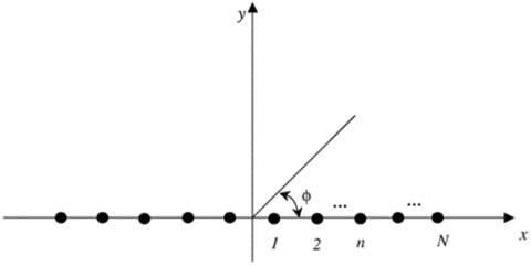
An antenna array is a collection of multiple antennas arranged in a particular pattern to accomplish desired characteristics such as enhanced gain, directivity, or beamforming. Figure 1 depicts a linear antenna array, which comprises of antennas arranged in a straight line [13].
When designing a linear antenna array, it is important to consider the spacing between the antennas, as this affects the array's performance. The spacing between adjacent antennas is typically chosen based on the desired radiation pattern and operating frequency [14].
Figure 1. Linear antenna array geometry
In antenna arrays, the array factor, also known as the radiation pattern or radiation field, describes how the radiated or received electromagnetic waves propagate in different directions from an antenna array. It represents the spatial distribution of the electromagnetic field strength or power radiation pattern in different directions.
The array factor is calculated by summing the contributions from each individual antenna element, taking into account the element's position, amplitude weight, and phase weight. The array factor is typically expressed as a function of the angle of radiation or direction of arrival [15].
For an LAA, the array factor can be represented mathematically as [16]:
$A F_{L A A}\left(I^L, \emptyset\right)=\sum_{n=-N_{L A A}}^{N_{L A A}} I_n^L \cos \left(k d_n^L \cos (\emptyset)\right)+\varphi_n^L$ (1)
where $\varphi_n, I_n, k$, and $x_n$ are the phase, excitation amplitude, wavenumber, and location of the $n^{\text {th }}$ element respectively. If we additionally assume that there is uniform amplitude and phase excitation $\varphi_n=0$ and $I_n=0$, It is possible to express the array factor as:
$A F(\varnothing)=2 \sum_{n=1}^N \cos \left[k x_n \cos (\varnothing)\right]$ (2)
The array factor equation considers the position of each antenna element and applies the appropriate phase shift based on the desired direction. The amplitude weights account for the relative strength or contribution of each antenna element to the overall radiation pattern.
By adjusting the amplitude weights and phase shifts of the individual antenna elements, it is possible to shape the radiation pattern of the linear antenna array. This allows for various applications such as steering the main beam in a specific direction, creating nulls or voids in certain directions to reduce interference, or achieving beamforming to focus the energy in a desired direction, the array factor provides valuable insights into the overall behavior of the linear antenna array and is an essential tool in antenna array design and analysis [17]. By minimizing the side lobes, a linear antenna array with Metaheuristics algorithms was used to achieve the best results [18]. This is accomplished by adjusting the parameters of each algorithm to specific values and preparing various antenna elements; the goal is to reduce the side lobes by varying the parameter values.
The SLL is a measure of the power or field strength in the sidelobes of the antenna's radiation pattern. sidelobes are lobes or peaks in the radiation pattern that occur in directions other than the main lobe (the primary direction of radiation). SLL quantifies the level of radiation in these sidelobes relative to the main lobe and is usually expressed in decibels (dB).
The objective of using an LAA is to enhance the beam pattern and decrease SLL. This is accomplished by identifying the optimal set of exciting currents for LAA elements, which is impossible without calculating the fitness function given by the following equation:
$ Fitness=\min \left(\max \left(20 \times \log _{10}\right)|A F(\emptyset)|\right)$ (3)
In the context of optimization algorithms, a fitness function is a mathematical function shown in Eq. (3). The performance of a linear antenna array is often evaluated based on its ability to focus or direct radiation in a specific direction (main lobe) while minimizing radiation in unwanted directions sidelobes. High-performance antenna arrays are designed to have low SLL, meaning that they minimize the power radiated in the sidelobes. The lower the SLL, the more focused and directional the antenna becomes, which is generally desirable for applications like radar, wireless communication, and beamforming [15].
The SLL is directly related to the characteristics of the array factor. Specifically, the SLL is a measure of the level of radiation in the sidelobes of the array factor. A low SLL indicates that the sidelobes of the array factor are suppressed, resulting in a more focused and directional main lobe.
In summary, the array factor, SLL, and the performance of a linear antenna array are interconnected. The design of the array, including element spacing and excitation, directly affects the radiation pattern and, consequently, the SLL. Minimizing SLL is essential for applications where precise beamforming and radiation control are critical [18].
Minimizing side lobes in the radiation pattern of an antenna is important for several reasons, and it provides several benefits, particularly in communication, radar, and other applications where precise radiation control is essential.
There are many algorithms that are used in different applications and in this paper the effect of the parameters of GA, FPA, and GWO algorithms will be recognized and the parameters changed when different numbers of antenna elements to minimize SLL.
3.1 Genetic algorithm
The genetic algorithm is an artificial evolution-based research algorithm [19]. Adopted research mechanisms frequently depend on the formulation and seek for adaptations involving alterations made to the initial algorithm, the effectiveness of this algorithm is dependent on these formulations.
Its operational mechanism comprises a collection of classified symbols and a token in the form of chromosomes, which collectively ascertain optimal solutions for groups in a more efficient manner than employing each symbol in isolation [20]. John Holland, a physicist, devised and proposed this evolutionary technology. The stages delineated are as follows: reconstruction initiation, evaluation, and selection. The principal phases comprise the last three. The initial stage involves the stochastic selection of chromosomes to ascertain the population size. Subsequently, an evaluation is conducted, during which the distinct fitness of each individual is ascertained and reassembled. This reassembling process identifies the progenitors and, based on the fitness of the progeny, the new chromosome. While mutation and crossover are considered crucial aspects in genetic algorithms, further clarification on these concepts can be provided at a later stage.
The Three values characterize θ venom, $\varnothing$ longitude, and radial distance, R (equivalent to the Earth's radius of approximately 6378100 meters), Utilized to ascertain the Coordinates in a sphere of a given point. Applying the following formula [21]:
$X=R \times \sin \theta \times \cos \emptyset$ (4)
$Y=R \times \sin \theta \times \sin \emptyset$ (5)
$Z=R \times \cos \theta$ (6)
X, Y, and Z are distinct chromosomal parameters that, when converted to 2D Fourier, generate images. For the purpose of enhancing the array composition, reference [22] utilized u-v with n(n-1) antennas by further enhancing frequency and decreasing SLL for the evolutionary algorithm. The first stage of the genetic algorithm consists of arbitrarily constructing chromosomes between longer and shorter at-length points to ensure appropriate annexation. After that, the process of evaluating the necessary level of physical fitness begins. The likelihood of crossover and mutation occurring in the subsequent generation is considered, and the identification and reconstruction procedure are subsequently determined using a subset of the chromosomes between them.
Crossover: A new chromosome is produced through the arbitrary severance of chromosomes at one or more positions (X, Y, or Z) by the crossover operator. At one or more points, the intersection may materialize. There is no new material production as a consequence of the intersection. It augments the mean fitness of subsequent generations within the population through the fusion of two pre-existing chromosomes, thus producing new chromosomes.
Mutation: The mutation that the evolutionary algorithm arbitrarily induces in the chromosome gene may affect X, Y, Z, or multiple ones. By introducing additional chromosomes into the population, the mutation expands the solution space. Randomly modifying genes on chromosomes [20].
This algorithm features a range of strengths and weaknesses. the strengths are: Wide Application, Global Search, Population Diversity, and Crossover and Mutation. Weaknesses are Computational Intensity, Parameter Sensitivity, and Convergence Speed.
GA with LAAs was used to reduce the side lobes and reach the optimal solution in regard to a variant sum of antenna elements by changing the values of the parameters of GA which include Generation, Maximum Stall Generation, and Population Size as they affect the decrease of SLL and will be given a simple glimpse of each.
3.1.1 Generation
In a GA, generations, also known as iterations or epochs, play a crucial role in the evolutionary process. Each iteration represents a cycle of selection, reproduction, and genetic operators that simulate the natural process of evolution to find an optimal solution to a problem.
The number of iterations affects the balance between exploration and exploitation in a GA. In the early iterations, the algorithm focuses more on exploration. As iterations progress, the algorithm gradually shifts towards exploitation, refining, and improving solutions within the promising regions already discovered [23].
It also affected the convergence with each iteration, the initial population contains a diverse set of individuals, and through the selection and reproduction process, the algorithm gradually narrows down the search space to the fittest individuals. As iterations proceed, the population typically converges towards a region of the solution space that contains optimal or near-optimal solutions. If the algorithm is allowed to run for too few iterations, it may not reach an optimal solution and may terminate prematurely.
The quality of solutions found by a GA generally improves with more iterations creating new offspring with potentially better fitness values. Through genetic operators like crossover and mutation, the algorithm introduces diversity and helps in exploring new regions of the solution space [23].
The number of iterations directly impacts depends on the complexity of the problem, computational resources, and the desired trade-off between solution quality and time constraints.
3.1.2 Population size
The population size is a critical parameter in a genetic algorithm, representing the number of individuals (candidate solutions) present in each generation. The population size has a significant effect on the performance and behavior of a genetic algorithm, the effects are Convergence Speed, Generally, a larger population size increases the convergence speed of a genetic algorithm. The algorithm can exploit more promising regions of the search space, leading to faster convergence toward optimal or near-optimal solutions. However, increasing the population size also incurs a higher computational cost per generation [14].
Exploration and exploitation are influential factors in GA, larger population size increases the diversity of the solutions explored in the search space. It allows for a broader exploration of the solution landscape. On the other hand, a smaller population size promotes exploitation by focusing on the fitter individuals and converging towards local optima. In addition. The population size directly affects the computational resources required to execute the genetic algorithm. As the fitness evaluation and genetic operators need to be applied to a larger number of individuals [24].
The population size influences the genetic diversity within the population. A larger population tends to maintain higher diversity since there are more individuals and a wider range of genetic information. This diversity can be advantageous, especially in complex optimization problems where maintaining diverse solutions can help avoid premature convergence and find better solutions. It is often recommended to start with a moderate population size and then adjust it based on performance analysis and convergence behavior [25].
3.1.3 Maximum stall generations
In a genetic algorithm, the maximum stall iterations (also known as stagnation iterations) refer to the maximum number of consecutive generations in which there is no improvement in the fitness of the population. It is used as a termination criterion to stop the algorithm if it is unable to make progress. the effect of the maximum stall iterations parameter in a genetic algorithm can vary depending on the specific problem and the characteristics of the population [26].
One of the important influences is termination, when the maximum stall iterations limit is reached, the algorithm terminates, considering that further iterations are unlikely to yield better results. This helps in stopping the algorithm from running indefinitely and saves computational resources. Performance can be an influential factor in Setting the maximum stall iterations too low can lead to premature termination, preventing the algorithm from finding good solutions. Conversely, setting it too high can result in unnecessary computational effort if the population has truly stagnated. It is important to strike a balance between exploration and exploitation based on the problem at hand [27].
To determine the appropriate value for the maximum stall iterations, it is often helpful to consider the characteristics of the problem domain, the expected convergence rate, and the computational resources available.
3.2 Flower pollination algorithm
Yang [28], introduced this algorithm as one of the metaheuristics methods that incorporates the propagation of blossoming plants as a determining factor. It has been widely implemented and is founded upon four foundational principles: Local inoculation utilizes subjective and biological pollination as opposed to bioavailability and cross-vaccination, which are global vaccination strategies, probability p, that signifies a proportion of localized immunization substituted for immunization global.
FPA comprises core parameters of Levy-flights based step size $L(\beta)$, population size $(N)$, scaling factor $\gamma$, Switching Probability $p$, and $\varepsilon \in[0,1]$, and a uniform distribution is commonly employed in local inoculation [9].
Random number selection determines global and local inoculation. If the switching probability p is low, a global inoculation is administered; otherwise, an administration of a local inoculation occurs.
The subsequent equations provide a mathematical illustration of flower uniformity and global pollination:
$x_i^{t+1}=x_i^t+\gamma L\left(g_{\text {best }}-x_i^t\right)$ (7)
where, $x_i^t$ is the solution vector $x_i$ at iteration $t, \gamma$ is a scaling factor to control step size, and $g_{\text {best }}$ is the current best solution. L This number represents the Levy flights-based step size; it is an estimate of the pollination intensity. The following mathematical expression represents local pollination:
$x_i^{t+1}=x_i^t+\varepsilon\left(x_i^t-x_k^t\right)$ (8)
where $x_k^t$ and $x_j^t$ are pollen from several blooms belonging to the same kind of plant. If $x_j^t$ and $x_k^t$ are chosen from the same population, this is comparable to a local random walk as $\varepsilon$ comes from a uniform distribution in $[0,1]$.
This algorithm features a range of strengths and weaknesses. the strengths are: Global Exploration, Parallelism, and ease of Implementation. Weaknesses are: Limited Local Search, Convergence Speed, and Sensitivity to Parameters.
There are many ways used to minimize side lobes, FPA with LAA is used to reduce SLL and energy concentration on the main lobe. A range of parameters can be changed for more than one value and for different antenna elements, namely, the number of iterations, population size, probability of switch for FPA, and flower attraction rate.
3.2.1 Iterations
Iterations, in the FPA, refer to the number of times the algorithm goes through the main steps of the optimization process. Each iteration involves the evaluation of the fitness of the flowers, pollen dissemination among the flowers, and updating the flower population based on the obtained fitness values.
The number of iterations influences the balance between exploration (diversification) and exploitation (intensification) of the search process. Initially, a higher number of iterations tend to favor exploration, allowing the algorithm to search a broader space. As the iterations progress, the focus gradually shifts towards exploitation, refining the solutions in promising regions. The proper balance depends on the problem and should be determined through experimentation [29].
The number of iterations can be used as a stopping criterion in the FPA. For instance, the algorithm may be terminated after reaching a predefined number of iterations or when a certain convergence criterion is met. The stopping criteria can be based on the improvement in the objective function value. Increasing the number of iterations directly affects the computational time required for the optimization process.
While more iterations may lead to better solutions. In practice, in an FPA, it is often necessary to experiment with different iteration counts to find an optimal balance between exploration and exploitation.
3.2.2 Population size
The population size in an FPA, refers to the number of flowers or potential solutions that exist in each generation of the algorithm. The population size is a crucial parameter in the FPA, and it has a significant impact on the algorithm's performance and convergence behavior. Here are some effects of population size in a flower pollination algorithm.
The population size directly affects the computational resources required by the algorithm. With a larger population, the algorithm needs to evaluate fitness values for more solutions and perform additional operations such as pollen dissemination and flower updating. This can result in increased computational time and memory requirements.
A small population size increases the risk of premature convergence. If the population size is too small, there may be limited diversity among the solutions, leading to convergence to local optima and hindering the algorithm's ability to explore the search space effectively. It is important to choose a population size that allows for sufficient exploration to avoid premature convergence [9]. The population size influences the balance between exploration and exploitation. A larger population size allows for more diverse solutions, promoting exploration of the search space. On the other hand, a smaller population size favors exploitation by focusing on refining and intensifying the search around promising solutions.
Determining the optimal population size for a flower pollination algorithm involves considering the necessity to experiment with different population sizes and assess their impact on convergence speed, solution quality, and computational efficiency to find the most suitable value [28].
3.2.3 Probability of switch for FPA
In an FPA, the probability parameter determines the likelihood of a flower undergoing pollination or interaction with other flowers. This probability, often referred to as the pollen transfer probability or pollination rate, here are some effects of the probability parameter in an FPA [9].
The probability parameter influences the balance between exploration and exploitation. A higher probability promotes more extensive exploration by increasing the chances of pollen transfer between flowers. This allows for a wider search of the solution space. On the other hand, a lower probability favors exploitation by focusing on intensifying the search around promising solutions, potentially leading to convergence to better optima.
The probability parameter influences the diversity of the population. A higher probability enhances diversity by promoting frequent interactions between flowers, which can prevent premature convergence and improve solution quality. Lower probabilities, however, may limit the diversity and increase the risk of convergence to suboptimal solutions. While the probability parameter indirectly affects the computational resources required by the algorithm [10].
The probability parameter affects the convergence speed of the algorithm. Higher probabilities facilitate faster convergence as they encourage more interactions and information exchange between flowers. This can lead to faster convergence towards better solutions. while the probability parameter is a tunable parameter that needs to be calibrated for specific optimization problems. In summary, the optimal choice of probability depends on the problem at hand, and finding the right value often requires empirical analysis and experimentation.
3.2.4 Flower attraction rate
In an FPA, the flowers' attraction rate is a parameter that determines the strength of attraction between flowers during the pollination process. This parameter influences how flowers exchange information and move towards potentially better solutions. Here are some effects of the flowers' attraction rate in an FPA. The rate of attraction impacts the convergence speed of the algorithm. A greater attraction rate facilitates a quicker convergence, as flowers are powerfully attracted to superior solutions. This can expedite the algorithm's convergence to optimal solutions, particularly when the search landscape contains steep gradients.
The attraction rate plays a role in achieving a proper balance between exploitation and exploration. Higher attraction rates tend to prioritize exploitation, which can be beneficial in problems where local optima are common. Lower attraction rates emphasize exploration, which can help in problems with complex landscapes and multiple global optima. In addition, the attraction rate is a tunable parameter that requires careful calibration for each specific problem. It is crucial to experiment with different values of the attraction rate to find the optimal setting that suits the problem's characteristics [10].
In summary, the optimal choice of the attraction rate depends on the problem's characteristics and the desired search behavior. It is important to experiment and fine-tune this parameter to achieve the best performance for a particular optimization problem.
3.3 Grey wolf optimizer
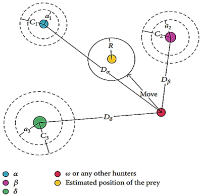
GWO is a metaheuristic algorithm that simulates the social hierarchy and hunting mechanisms of grey wolves. The order of grey wolf species is as follows: The male and female leaders are known as alphas $(\alpha)$. The second level of the wolf hierarchy consists of beta $(\beta)$ wolves, followed by delta $(\delta)$ wolves, and the lowest-ranking grey wolves are omega $(\omega)$. Mathematically, the hierarchy of grey wolves is modeled by considering $\alpha$ to be the optimal solution, the second in sequence $\beta$, followed by $\delta$, respectively. It is supposed that the candidate solutions are ω.
Consist of the primary phases of grey wolf hunts [29], Tracking, pursuing, and moving on the prey, and then pursuing, surrounding, and harassing the target until it ceases to move. finally, the predator attacks the prey. The behavior of encircling is mathematically represented by Eq. (10) [30]:
$\vec{D}=\left|\vec{C} \cdot \overrightarrow{X_p(t)}-\overrightarrow{X(t)}\right|$ (9)
$\vec{X}(t+1)=\overrightarrow{X_p}(t)-\vec{A} \cdot(\vec{D})$, (10)
where, $\vec{A}$ and $\vec{C}$ are vectors of coefficients, $\vec{X}$ represents the vector position of a grey wolf, $t$ denotes the current iterations, and $\overrightarrow{X_p}$ is the vector representing the position of the prey. Calculating the vectors $\vec{A}$ and $\vec{C}$ using:
$\vec{A}=2 \vec{a} \cdot \overrightarrow{r_1}-\vec{a}$, (11)
$\vec{C}=2 \cdot \overrightarrow{r_2}$, (12)
where, component of $\overrightarrow{r_1}, \overrightarrow{r_2}$ are random vectors in $[0,1]$ and $\vec{a}$ iteratively decrease linearly from 2 to 0 . In the GWO algorithm, $\alpha, \beta$, and $\delta$ guide the hunting (optimization). The canines $\omega$ are following these three wolves. The $\alpha, \beta$, and $\delta$ wolves are believed to have a greater understanding of the prospective locations of prey. Therefore, the first three best solutions are preserved, and the other search agents update their positions based on the best search agent's position. For this purpose, the following equations are utilized [30]:
$\begin{gathered}\overrightarrow{D_\alpha}=\left|\overrightarrow{C_1} \cdot \overrightarrow{X_\alpha}-\vec{X}\right|, \\ \overrightarrow{D_\beta}=\left|\overrightarrow{C_2} \cdot \overrightarrow{X_\beta}-\vec{X}\right|, \\ \overrightarrow{D_\delta}=\left|\overrightarrow{C_3} \cdot \overrightarrow{X_\delta}-\vec{X}\right|, \\ \overrightarrow{X_1}=\overrightarrow{X_\alpha}-\overrightarrow{A_1} \cdot\left(\overrightarrow{D_\alpha}\right), \\ \overrightarrow{X_2}=\overrightarrow{X_\beta}-\overrightarrow{A_2} \cdot\left(\overrightarrow{D_\beta}\right), \\ \overrightarrow{X_3}=\overrightarrow{X_\delta}-\overrightarrow{A_3} \cdot\left(\overrightarrow{D_\delta}\right), \\ \vec{X}(t+1)=\frac{\overrightarrow{X_1}+\overrightarrow{X_2}+\overrightarrow{X_3}}{3},\end{gathered}$ (13)
Using Eq. (13), a search agent adjusts its position according to $\alpha, \beta$, and $\delta$ in the n-dimensional search space as depicted in Figure 2. In addition, the final position would be at a random location within the search space defined by the coordinates of $\alpha, \beta$, and $\delta$. Consequently, estimate the position of the prey, whereas other wolves update their coordinates arbitrarily around the prey [30].
Figure 2. Position update in GWO
This algorithm features a range of strengths and weaknesses. the strengths are: Effective Exploration, Fewer Parameters, and Fast Convergence. Weaknesses are: Limited Research, Lack of Diversity, and Limited Application.
This algorithm has been used with LAA which is used to reduce the side lobes and make the largest amount of energy be in the main lobe as well as the role of fitness objective function the effect of parameters plays an important role in the decrease of SLL.
3.3.1 Iterations
The number of iterations in the GWO algorithm, also known as the maximum number of generations, is a crucial parameter that affects the algorithm's performance. Generally, increasing the number of iterations allows the algorithm to explore the search space more extensively, potentially leading to better solutions [10].
The optimal number of iterations can vary depending on the complexity of the problem being solved. Simple problems may converge quickly, requiring fewer iterations, while highly complex problems may need a larger number of iterations to reach satisfactory solutions.
The GWO algorithm aims to strike a balance between exploration (searching the solution space for promising regions) and exploitation (refining the solutions around the identified regions). Increasing the number of iterations allows for more exploration, but there's a risk of spending excessive time searching unfruitful areas without sufficient exploitation [31].
Typically, the GWO algorithm exhibits convergence behavior, meaning that the quality of solutions improves with iterations initially and then reaches a relatively stable state. Once the algorithm converges, further iterations may not significantly improve the solutions.
In summary, the number of iterations in the GWO algorithm plays a significant role in the algorithm's performance. Finding the optimal number of iterations often involves experimentation, considering the problem's complexity and available computational resources.
3.3.2 Population size
The population size is a critical parameter in the GWO algorithm, as it determines the number of candidate solutions or "wolves" in each generation. The population size can have a significant impact on the algorithm's performance and convergence characteristics.
The population size directly affects the memory consumption of the GWO algorithm. As the population size increases, the memory requirement to store the candidate solutions also increases. On the other hand, a very large population size can lead to premature convergence, where the algorithm settles around a suboptimal solution too early in the optimization process. This occurs when the wolves in the population converge too quickly and do not explore the search space effectively [32].
Increasing the population size in the GWO algorithm directly affects the computational time required for each generation. With more wolves, the fitness evaluation of the candidate solutions and the update process becomes computationally more expensive.
Determining an appropriate population size for the GWO algorithm involves considering experiments with different population sizes and analyzing the convergence behavior and solution quality to find the optimal value for a particular problem.
In conclusion, the choice between GA, FPA, GWO, depends on the specific characteristics of the optimization problem at hand. GAs is versatile and widely applicable but require careful parameter tuning. FPA is simple and efficient for global exploration but may lack precision in local search. GWO offers fast convergence but may not perform well in all problem domains. Successful application often depends on the problem's nature, available computational resources, and the need for global or local optimization.
Each algorithm is influenced by a set of parameters that in turn affect the performance of the algorithm. Each parameter was tested separately and for a different number of antenna elements (N = 8,16,32,64,128,256) to see its impact on the performance of the algorithm, how much SLL attrition and the concentration of the greatest amount of energy on the main lobe, using the simulation software MATLAB version 2020.
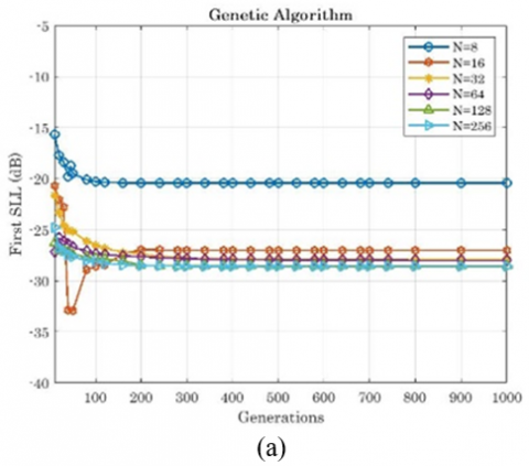
One of the most important influential parameters in GA is the generation shown in Figure 3(a), where it has been tested for a range of different values and found at N = 8 The effect of the iteration is very little on the decrease of SLL so that it is best valued at iteration 240 and SLL is reduced by -20.4335dB. At N = 16 starts, the effect is very small at generation 35, but after this generation, there is a fluctuation of SLL to the maximum at iteration 50 and a value of -32. 9533dB.
When (N = 32,64,128,256) the effect of iteration is very low, there is a slight, negligible oscillation so that it is the best SLL at iterations 900,680,1000 and with values of -27.8764dB, -28.0044dB, -28.5568dB, -28.6204dB respectively.
Another effect is the population size Figure 3(b), which influences the SLL values and is found at N = 8, A slight fluctuation occurs when the population size is 120 and beyond, that is when the population size is 140, there is the greatest decrease of SLL to -21.8781dB. At N = 16 the effect of population size 280 is the best because it has a decrease of -27.1949dB and before that the effect is minimal.
At (N = 32,64,128,256) the effect is negligible and the largest decrease has been SLL at 200 population size and at -27.8764dB, -28.0044dB, -28.5568dB and-28.6204dB respectively. They are the same values when generation 1000.
Maximum stall generation is an influencer in GA as shown in Figure 3(c) in N = 8,32 found to be the best diminishing SLL when Max stall generation is 13 and valued at -20.4335dB, -27.8756dB respectively.
At N = 16 SLL decreases to a maximum of -28. 5039dB at Max stall generation is 7. At N = 64,256 the best SLL values are -28.0044dB and-28.6204dB respectively and at Max stall generation 50.
Figure 3. (a). Iteration, (b). Population size, (c). Maximum stall iterations
Table 1. Shows the best results of SLL reduction by GA
|
Max Peak SLL |
Number of Elements |
Parameter Effects |
|
-32.9523 dB |
16 |
Generation 50 |
|
-28.6204 dB |
256 |
Population size 200 |
|
-28.6204 dB |
256 |
Max stall generation 50 |
Table 1 shows the impact of parameters on the reduction of SLL to the maximum extent possible. This effect has proven that the signal will be highly efficient and with the greatest amount of signal-to-noise ratio.
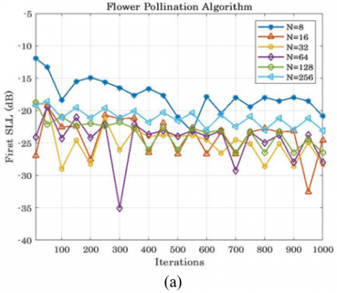
In FPA, many tests were conducted to determine the impact of the parameters on each. iteration is an important effect. It was tested on more than one value and for a different number of antenna elements.
Figure 4. (a) Iteration, (b) Population size, (c) Probability, (d) flower attraction rate
Figure 4(a) shows At N = 8, the best iteration was found at 550, where he reduced SLL to -23.2012dB. At N = 16,32, SLL was found to have decreased to the greatest amount, at 950 and 100 in the values of -32.5694dB and -29.0334 dB, respectively. At N = 64,128,256, the best values for SLL were at iterations of 300,700,100, reducing it to -35.0696dB, -26.4663dB, and -23.0646dB, respectively.
The population size of the parameters tested with a set of values is found at N = 8,16 SLL decreased to the maximum at the population size of 80 and 160 at -23.3463dB and -34.5790dB respectively. For other population sizes, it has a slight effect. At N = 32,64, the best test for population size was at 100 and 200, where SLL was reduced to -28.5110dB and -28.0148dB respectively. At N = 128,256, SLL decreased to the best amount at a population size of 200,280 and -26.4663dB and -25.4162dB respectively. As see in Figure 4(b).
The probability is one of the parameters on which the tests were performed and the use of more than infinite as shown in Figure 4(c) at N = 8,16 at first, the probability effect is very small, but at probability 1 and 0.7 the SLL is the best value at -34.9451dB and-31.6000dB respectively. either at N = 32,64, the amount of change is very little and the best values of SLL are at probability 0.8 and at values -28.3071dB and -28.0148dB respectively.
At N = 128,256 the probability has a very slight effect and is negligible except when the probability is 0 .1 and 0.2 the SLL has decreased to -27.8910dB and-25.1216dB respectively.
In Figure 4(d) the flower attraction rate is well influenced in N = 8,16,32. The effect is found to be good and its best value at 3,0.5,0.5 and SLL decreased to -26,9941dB -33.2830dB and-28.8755dB respectively.
When N = 64,128,256 flower attraction effect is wobbly, find that the best values of SLL are -28.0148dB, -26.4663dB, -24.0355dB and at the rate of attracting flowers 1, 1.5 and 1.5 respectively.
Table 2. Shows the best results of SLL reduction by FPA
|
Max Peak SLL |
Number of Elements |
Parameter Effects |
|
-35.0696 dB |
64 |
Iteration 300 |
|
-34.5790 dB |
16 |
Population size 160 |
|
-34.9451 dB |
8 |
Probability 1 |
|
-33.2830 dB |
16 |
Attraction flower rate 0.5 |
Table 2 shows the impact of parameters on the reduction of SLL to the maximum extent possible. This effect has proven that the signal will be highly efficient and with the greatest amount of signal to noise ratio
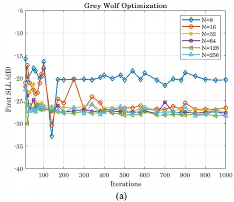
In GWO several tests were conducted to see the impact of parameters on the performance of the algorithm. In the iteration effect a number of values were tested and for a different of antenna elements in N = 8,16 was found to have a varying effect up to 100 iterations either at repeat 140 SLL dropped to a maximum amount of -32.8479dB, -30.4126dB respectively. At N = 32.64 the effect of repetition is oscillating as SLL is reduced to -27.3854dB, and -27.8503dB at repeat 1000 and 660 respectively. At N = 128,256, SLL has been minimized at 20, 850dB to -30.0366dB and -28.3399dB respectively.as shown in Figure 5(a).
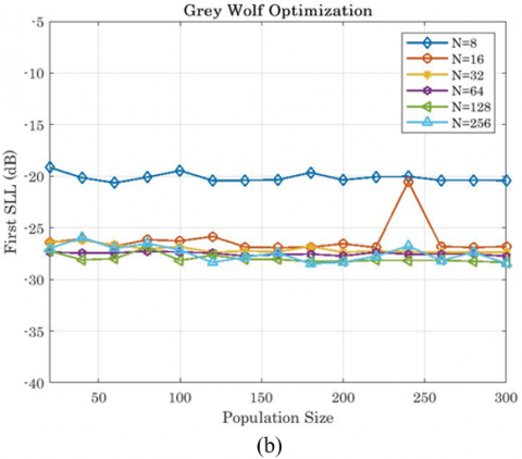
The size of the population as shown in Figure 5(b) at N = 8 has a varying effect at the size of the population 60 reduced SLL to -20.6427dB. At N = 16,32 the effect of population size at 160 and 280 is oscillating, reducing SLL to -26.9255dB and -27.3898 respectively. At N = 64,128,256, SLL was maximized at values -27.7516dB, -28.3581dB, and -28.4846dB at population sizes 300,300,180 respectively.
Figure 5. (a). Iteration, (b). Population size
Table 3. Shows the best results of SLL reduction by GWO
|
Max Peak SLL |
Number of Elements |
Parameter Effects |
|
-32.8479 dB |
8 |
Iteration 140 |
|
-28.4846 dB |
256 |
Population size 180 |
Table 3 shows the impact of parameters on the reduction of SLL to the maximum extent possible. This effect has proven that the signal will be highly efficient and with the greatest amount of signal-to-noise ratio.
Achieving lower SLL values is essential in various applications where precise control of signal directionality, reduced interference, improved signal quality, and compliance with regulatory standards are important. Lower SLL values can enhance the overall performance and reliability of communication, radar, and other systems that rely on antenna radiation patterns.
Table 4 shows the difference between the results presented in this paper and the results of previous literature and shows that the results of this paper are best caused by the difference of objective function or the different order of arrays as well as the different number of antenna elements and different values of parameters for each algorithm, so this research is continuing because it didn't limit changing parameters to a certain number, but it is compared between them to get to the best solution by reducing SLL to the maximum amount.
Table 4. Illustrates the results of previous literature
|
Ref. |
Algorithms |
Effects Parameters |
Number of Elements |
Best Reduction SLL |
|
[32] |
GA |
Iteration 200 |
N=20 |
-9.9776 dB |
|
[33] |
GA GWO |
Iteration 10 Iteration 10 |
N=52 N=24 |
-29.0200 dB -48.9600 dB |
|
[34] |
FPA |
Iteration 500 Population size 40 Probability 0.5 |
N=16 |
-35.2100 dB |
By implementing the three algorithms GA, FPA, and GWO on an antenna array comprising varying numbers of elements, it is feasible to deduce that energy can be concentrated in the main lobe, thereby preventing misdirection of energy into the side lobes.
The best value when using GA and when repeat is the effect is at 16-element SLL decreases to -32.9523dB and at 50 iterations. When using the FPA and the parameter itself is the influencer, 64-element is the best as SLL reduced to -35.0696dB at iteration 300. When using GWO and iteration is the effect the best iteration is 140 where SLL is reduced to -32.8479dB and at 8-element.
When the population size is taken as an influential parameter and using GA, the best value is at 256-element where SLL is reduced to -28.6204dB and at the size of the population of 200. When using FPA, the best values are at 16-element -34.5790dB and a population size of 160. In GWO the best values are at 256-element at 180 population size where SLL is reduced to -28.4846dB.
When it is the max stall iteration of an influencer, then GA has the best values at 256-element -28.6204dB and at max stall iteration 50. The probability is an influential parameter in FPA. It was concluded that the best values are at probability 1 at 8-element, where SLL reduced to -34.9451dB. As for the effect of the flower attraction rate, the best values at the rate of 0.5 and the reduction of SLL to 33.2830dB at 16-element
Studies continue to this day to see the impact of parameters and the possibility of changing their values as well as the changing function of fitness on the performance of algorithms.
Use other algorithms to know the impact of their parameters on SLL reduction.
Using the objective function is different because its difference affects the reduction of SLL and therefore changes the impact of parametrizes on them.
I would like to thank prof. Dr. Saad S. Hreshee supporting my work.
|
AF |
Array factor |
|
γ |
Scaling factor |
|
L |
Levy Figurehts |
|
gbest |
current best solution |
[1] Schmidhuber, J. (2015). Deep learning in neural networks: An overview. Neural Networks, 61: 85-117. https://doi.org/10.1016/j.neunet.2014.09.003
[2] Blum, C., Merkle, D. (Eds.). (2008). Swarm intelligence: Introduction and applications. Springer Science & Business Media.
[3] Luo, X., Wang, J., Li, X. (2017). Joint grid network and improved particle swarm optimization for path planning of mobile robot, In 2017 36th Chinese Control Conference (CCC), Dalian, China, pp. 8304-8309. https://doi.org/10.23919/ChiCC.2017.8028672
[4] Clerc, M. (2010). Particle swarm optimization. Vol. 93. John Wiley & Sons.
[5] Shi, Y., Eberhart, R. (1998). A modified particle swarm optimizer. In 1998 IEEE international conference on evolutionary computation proceedings. IEEE World Congress on Computational Intelligence, Anchorage, AK, USA, pp. 69-73. https://doi.org/10.1109/ICEC.1998.699146
[6] Dorigo, M., Maniezzo, V., Colorni, A. (1996). Ant system: optimization by a colony of cooperating agents. IEEE Transactions on Systems, Man, and Cybernetics, Part B (Cybernetics), 26(1): 29-41. https://doi.org/10.1109/3477.484436
[7] Yang, X.S. (2010). Nature-inspired metaheuristic algorithms. Luniver Press.
[8] Sun, G., Liu, Y., Li, H., Liang, S., Wang, A., Li, B. (2018). An antenna array sidelobe level reduction approach through invasive weed optimization. International Journal of Antennas and Propagation, 1-16. https://doi.org/10.1155/2018/4867851
[9] Saxena, P., Kothari, A. (2016). Linear antenna array optimization using flower pollination algorithm. SpringerPlus, 5: 1-15. https://doi.org/10.1186/s40064-016-1961-7
[10] Mirjalili, S., Mirjalili, S.M., Lewis, A. (2014). Grey wolf optimizer. Advances in Engineering Software, 69: 46-61. https://doi.org/10.1016/j.advengsoft.2013.12.007
[11] Srinivas, M., Patnaik, L.M. (1994). Adaptive probabilities of crossover and mutation in genetic algorithms. IEEE Transactions on Systems, Man, and Cybernetics, 24(4): 656-667. https://doi.org/10.1109/21.286385
[12] Das, S., Suganthan, P.N. (2010). Differential evolution: A survey of the state-of-the-art. IEEE transactions on evolutionary computation, 15(1): 4-31. https://doi.org/10.1109/TEVC.2010.2059031
[13] Balanis, C.A. (2016). Antenna theory: Analysis and design. John Wiley & Sons.
[14] Israa, M., Hreshee, S.S. (2018). Reduction of side lobe level in a time-modulated linear array using invasive weed optimization and particle swarm optimization. Journal of Engineering and Applied Sciences, 13: 11048-11054.
[15] Asaad, H., Hreshee, S.S. (2022). A review about the optimization algorithm for SLL reduction in PAA. 2022 3rd information technology to enhance e-learning and other application (IT-ELA), Baghdad, Iraq, pp. 215-221. https://doi.org/10.1109/IT-ELA57378.2022.10107948
[16] Sharaqa, A., Dib, N. (2014). Design of linear and elliptical antenna arrays using biogeography based optimization. Arabian Journal for Science and Engineering, 39: 2929-2939. https://doi.org/10.1007/s13369-013-0794-8
[17] Lafta, N.A., Hreshee, S.S. (2021). Wireless sensor network’s localization based on multiple signal classification algorithm. International Journal of Electrical and Computer Engineering, 11(1): 498-507. https://doi.org/10.11591/ijece.v11i1.pp498-507
[18] Andersen, J. B. (2000). Antenna arrays in mobile communications: Gain, diversity, and channel capacity. IEEE antennas and Propagation Magazine, 42(2): 12-16. https://doi.org/10.1109/74.842121
[19] Sampson, J.R. (1976). Adaptation in Natural and Artificial Systems (John H. Holland). https://doi.org/10.1137/1018105
[20] Katoch, S., Chauhan, S.S., Kumar, V. (2021). A review on genetic algorithm: Past, present, and future. Multimedia tools and applications, 80: 8091-8126. https://doi.org/10.1007/s11042-020-10139-6
[21] Kiehbadroudinezhad, S., Noordin, N.K., Sali, A., Abidin, Z.Z. (2014). Optimization of an antenna array using genetic algorithms. The Astronomical Journal, 147(6): 147. https://doi.org/10.1088/0004-6256/147/6/147
[22] Eiben, A.E., Smith, J.E. (2015). Introduction to evolutionary computing. Springer-Verlag Berlin Heidelberg.
[23] Guo, J., Xue, P., Zhang, C. (2021). Optimal design of linear and circular antenna arrays using hybrid GWO-PSO algorithm. In 2021 3rd International Academic Exchange Conference on Science and Technology Innovation (IAECST) Guangzhou, China, pp. 138-141. https://doi.org/10.1109/IAECST54258.2021.9695624
[24] Goldberg, D.E. (1989). Genetic algorithms in search, optimization, and machine learning. Addison-Wesley Professional. Chapter 4.1 Explores the Relationship Between Population size and Convergence Speed.
[25] Smith, J.D., Johnson, A.B. (2018). Stagnation detection and termination criteria for genetic algorithms. IEEE Transactions on Evolutionary Computation, 22(2): 282-293.
[26] Holland, J.H. (1992). Adaptation in natural and artificial systems: An introductory analysis with applications to biology, control, and artificial intelligence. MIT Press.
[27] Yang, X.S., Karamanoglu, M., He, X. (2014). Flower pollination algorithm: A novel approach for multiobjective optimization. Engineering Optimization, 46(9): 1222-1237. https://doi.org/10.1080/0305215X.2013.832237
[28] Yang, X.S. (2012). Flower pollination algorithm for global optimization. In International Conference on Unconventional Computing and Natural Computation, Orléans, France, pp. 240-249. https://doi.org/10.1007/978-3-642-32894-7_27
[29] Bairwa, S.K., Kumar, P., Baranwal, A.K. (2016). Enhancement of radiation pattern for linear antenna array using Flower Pollination Algorithm. In 2016 International Conference on Electrical Power and Energy Systems (ICEPES) Bhopal, India, pp. 1-4. https://doi.org/10.1109/ICEPES.2016.7915896
[30] Cai, Z., Gu, J., Luo, J., Zhang, Q., Chen, H., Pan, Z., Li, Y., Li, C. (2019). Evolving an optimal kernel extreme learning machine by using an enhanced grey wolf optimization strategy. Expert Systems with Applications, 138: 112814. https://doi.org/10.1016/j.eswa.2019.07.031
[31] Salgotra, R., Singh, U., Sharma, S. (2020). On the improvement in grey wolf optimization. Neural Computing and Applications, 32: 3709-3748. https://doi.org/10.1007/s00521-019-04456-7
[32] Shen, G., Liu, Y., Sun, G., Zheng, T., Zhou, X., Wang, A. (2019). Suppressing sidelobe level of the planar antenna array in wireless power transmission. IEEE Access, 7: 6958-6970. https://doi.org/10.1109/ACCESS.2018.2890436
[33] Rezagholizadeh, H., Gharavian, D. (2018). A thinning method of linear and planar array antennas to reduce SLL of radiation pattern by GWO and ICA algorithms. AUT Journal of Electrical Engineering, 50(2): 135-140. https://doi.org/10.22060/eej.2018.13697.5182
[34] Almagboul, M.A., Shu, F., Qian, Y., Zhou, X., Wang, J., Hu, J. (2019). Atom search optimization algorithm based hybrid antenna array receive beamforming to control sidelobe level and steering the null. AEU-International Journal of Electronics and Communications, 111: 152854. https://doi.org/10.1016/j.aeue.2019.152854