Abdelhak Ouanane*![]() | Nacereddine Djelal
| Nacereddine Djelal![]() | Fares Bouriachi
| Fares Bouriachi![]()
© 2023 IIETA. This article is published by IIETA and is licensed under the CC BY 4.0 license (http://creativecommons.org/licenses/by/4.0/).
OPEN ACCESS
Cardiovascular diseases pose a significant global health challenge, emphasizing the need for improved techniques in early detection and diagnosis. This study focuses on enhancing the classification of cardiovascular diseases by optimizing an LSTM-based model using the Ant-lion algorithm. In order to achieve this, we utilize the Local Binary Patterns (LBP) technique for feature extraction, which captures important patterns in electrocardiography (ECG) data. The Ant-lion algorithm is then employed to optimize the LSTM model and improve its performance. To evaluate the proposed methodology, we selected the widely used MIT-BIH Arrhythmia Dataset. This dataset contains a variety of heart disease cases, enabling comprehensive testing and validation. In addition to accuracy, we assess various quantitative metrics such as precision, recall, and F1-score to provide a more comprehensive evaluation of the model's performance. This research contributes to the field of ECG classification by highlighting the potential of combining deep learning models with meta-heuristic algorithms. The findings validate the effectiveness of our approach on the MIT-BIH Arrhythmia Dataset, reinforcing the importance of further exploring such optimization techniques in cardiovascular disease diagnosis and management.
electrocardiogram, heart disease, LBP, LSTM, ALOA, meta-heuristic
The heart, an integral organ, acts as the fulcrum that propels the functionality of the human organism. Its role in ensuring the circulation of oxygen and nutrients via the bloodstream is paramount. Yet, it is not impervious to certain conditions that can impede its normal functionality. According to the World Health Organization, cardiovascular diseases have emerged as the primary cause of mortality worldwide, with an estimated 17 million deaths recorded annually. These diseases are predominantly associated with the following factors:
·Hypertrophy of the myocardium.
·The increase in blood pressure.
·Irreversible anemia due to kidney problems.
There is thus an urgent need to give serious thought to the development of more appropriate techniques to assist cardiologists, to screen for possible heart disease and/or to search for diseases that are not yet recognized and to adopt available solutions.
Electrocardiography is one of the medical sciences, to record and interpret the electrical activity of the patient's heart. This electrical activity is linked to potential changes in heart cells. Many researchers have been interested in the diagnosis using image-processing techniques.
Mohamed et al. [1] proposes a real-time ECG image classification system using Haar-like features and artificial neural networks. The authors use a training set of 100 ECG images and a test set of 50 ECG images. The system achieves a classification accuracy of 99% on the test set. The authors also evaluate the system's performance in terms of speed and robustness. The system is able to classify ECG images in real time and is robust to noise and variations in the ECG signal.
Zubair et al. [2], proposes an automated ECG beat classification system using convolutional neural networks (CNNs). The authors use a CNN to extract features from ECG signals. The CNN is then trained on a dataset of ECG signals with known beat types. The authors evaluate the performance of the CNN on a test set of ECG signals. The CNN achieves an accuracy of 97% in classifying ECG beats. Acharya et al. [3] introduces a deep CNN model designed to classify different types of heartbeats in ECG signals automatically. With high accuracy in diagnostic classification, the model shows promise for efficiently identifying arrhythmic heartbeats, making it a valuable tool for screening purposes. The study emphasizes the effectiveness of the proposed CNN model in accurately detecting and categorizing various types of heartbeats in ECG signals. Kachuee et al. [4] presents a deep learning approach for classifying ECG heartbeats. The authors use a deep transfer learning model to classify ECG heartbeats. The model is trained on a dataset of ECG heartbeats with known labels. The authors evaluate the performance of the model on a test set of ECG heartbeats. The model achieves an accuracy of 98% in classifying ECG heartbeats. Izci et al. [5] presents a deep learning technique for detecting cardiac arrhythmias from 2D ECG images. The authors use a convolutional neural network (CNN) to extract features from the ECG images. The CNN is then trained on a dataset of ECG images with known arrhythmias. The authors evaluate the performance of the CNN on a test set of ECG images. The CNN achieves an accuracy of 98% in detecting cardiac arrhythmias.
Serhani et al. [6] provides a review of ECG monitoring systems. The authors discuss the different types of ECG monitoring systems, their architectures, and their processes. The authors also discuss the key challenges in ECG monitoring systems. Bharti et al. [7] presents a machine learning and deep learning approach for predicting heart disease. The authors use a combination of logistic regression, support vector machines, and deep neural networks to predict heart disease from a dataset of patient medical records. The authors evaluate the performance of the models on a test set of patients. The models achieve an accuracy of 92% in predicting heart disease.
Building upon the existing foundation, recent works in cardiovascular disease research employ deep learning techniques to further enhance diagnostic accuracy and improve prediction capabilities. These advancements contribute to the ongoing efforts of addressing the challenges in cardiovascular disease diagnosis and offer promising avenues for improved patient care.
Khan et al. [8] investigate the prediction of cardiovascular diseases using machine learning algorithms. They propose a novel approach that combines different machine learning techniques to improve prediction accuracy. The study explores the application of these algorithms in the context of healthcare, aiming to enhance early detection and prevention of cardiovascular diseases.
Subramani et al. [9] presents a research study on the prediction of cardiovascular diseases using a combination of machine learning and deep learning techniques. The authors leverage the power of deep learning algorithms to extract meaningful patterns from large-scale medical data and integrate them with traditional machine learning algorithms for accurate disease prediction. The paper highlights the potential of incorporating deep learning methods in cardiovascular disease prediction and emphasizes the importance of early diagnosis for effective intervention.
Garcia-Ordás et al. [10], employ feature augmentation to enhance the predictive capabilities of their deep learning model. By integrating a diverse set of features and leveraging the power of deep learning algorithms, the study aims to improve the accuracy and reliability of heart disease risk prediction. The paper highlights the potential of deep learning techniques for risk assessment in cardiovascular health.
Zhao [11] provides a comprehensive review of transformer-based deep learning models in the context of ECG diagnosis for cardiovascular disease detection. The author explores the capabilities of transformer architectures in capturing temporal dependencies and extracting relevant features from ECG signals. The review discusses the advantages, limitations, and potential applications of transformer-based models for improving the accuracy and efficiency of cardiovascular disease diagnosis using ECG data.
In the light of the aforementioned state of the art, we can propose our main contribution as follow:
·We have used the LBP technique to extract geometric and local features.
·LBP features are fed the LSTM-based model.
·LSTM-based model to predict diseases classes taking into account the estimation of the waves P, R, Q, S, T.
Improving the optimizer of the LSTM using meta-heuristic algorithms.
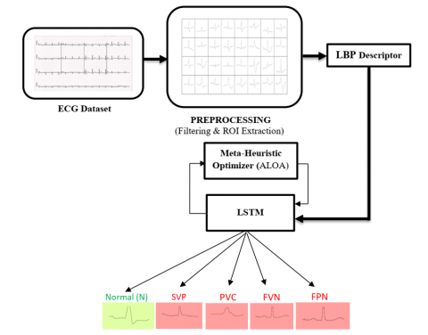
The proposed early diagnosis system is illustrated in Figure 1 and consists of five main phases:
The first phase describes the ECG standard dataset. The second is the preprocessing phase, which focuses on improving image quality, extracting and resizing the region of interest. The third stage involves features extraction using the LBP algorithm to generate ECG signatures. These serve as input vectors to train the LSTM-based model which combined with a meta-heuristic algorithm to optimize its convergence and improve its performance. Finally, various tests will be carried out in order to categorize the diseases classes and perform the proposed system using various metrics.
Figure 1. Synoptic scheme of the proposed system
2.1 Dataset
In order to validate the proposed diagnosis system, we have used MIT-BIH Arrhythmia Dataset [12, 13], which is composed of 109445 ECG images. The dataset contains five classes: Normal (N), Supra-ventricular premature (SVP), Premature ventricular contraction (PVC), Fusion of ventricular and normal (FVN) and Fusion of paced and normal (FPN) according to the association for the advancement of medical instrumentation recommendations (AAMI).
2.2 Pre-processing
The different images of over-mentioned dataset contain noises and insignificant objects and textures like the profiling header, dates and digits must be removed in order to extract the region of interest (ROI) which only contains the ECG signal. First, an Otsu binarization technique is performed to extract the mask where its coordinates are predefined beforehand and then the original image is overlaid with the mask to extract the region of interest resized to 128x128 of resolution. Then, a median filter is used to enhance the image quality.
2.3 LBP descriptor
LBP is a descriptor that used to describe the local features of an image. LBP has important advantages such as grayscale stability and spin stability. It was proposed by Ojala et al. [14, 15]. Due to the easy calculation and accurate impact of LBP functions, they have been extensively used in lots of fields of computer vision. Application, LBP feature comparison is a well-known application for face recognition and target detection.
Consider the 3×3 binary mask as shown in Figure 2. The value of the center must be compared to the neighbored pixel values if the value of the adjacent pixel is greater than the central pixel, the new value becomes 1, and otherwise it is 0. These 8-bit binary numbers are organized in collection to shape a binary number. This binary number is the LBP value of the central pixel. The LBP value of the middle pixel reflects the texture information of the area around the pixel.
Figure 2. LBP process
The LBP can be described as follow:
$\operatorname{LBP}\left(x_c, y_c\right)=\sum_{P=0}^{P-1} 2^P S\left(i_P-i_c\right)$ (1)
where, (xc, yc): Denotes central pixel, ic: The pixel intensity, ip: Presents the neighbor pixel intensity.
The sign function is given by:
$S(x)=\left\{\begin{array}{lr}1 & \text { if } x \geq 0 \\ 0 & \text { else }\end{array}\right.$ (2)
The LBP features for each extracted ECG image can be summarized into a signature vector. The latter, need to be normalized and rescaled to the range [-1, 1] to fed the LSTM model.
2.4 LSTM model
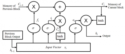
A long-short term memory [16] is a specific type of recurrent neural network [17]. It avoids the problem of long-term dependency through intentional design unlike to all RNNs that have a sequential form of repeating neural network units.
In standard RNN, this repeating unit has a very simple structure, such as the Tanh layer. LSTM has the same architecture, but the repeating modules have a different architecture. Unlike to a single neural network layer, there are four layers, which interact in a very special way as mentioned in Figure 3.
Figure 3. LSTM Architecture
where, ht: Output of the current layer, ht-1: Denotes output of the previous layer, xt: is the current input, Ct: Denotes the cell state of the current layer, Ct-1: Denotes the cell state of the previous layer, ft: Denotes the forget gate layer, $\tilde{C}_t$: Denotes the candidate vector.
We can define the system by introducing the forget gate layer given by:
$f_t=\sigma\left(W_f \cdot\left[h_{t-1}, x_t\right]+b_f\right)$ (3)
where, σ: is the sigmoid function, Wf: is the weights of the forget layer, bf: is the bias of the forget layer.
Then we update the input layer using the following equations:
$i_t=\sigma\left(W_i \cdot\left[h_{t-1}, x_t\right]+b_i\right)$ (4)
where, it: is the output of the input gate layer, Wi: is the weights of the input gate layer, bi: is the bias of the input gate layer.
$\widetilde{C}_t=\tanh \left(W_C \cdot\left[h_{t-1}, x_t\right]+b_C\right)$ (5)
where, $\tilde{C}_t$: is the output of the input candidate layer, tanh: is the output of the input candidate layer, WC: is the hyperbolic tangent function, bC: is the bias of the candidate layer
The output layer given ass follow:
$o_t=\sigma\left(W_o \cdot\left[h_{t-1}, x_t\right]+b_o\right)$ (6)
where, ot: is the output of the output gate layer, Wo: is the weights of the output gate layer, bo: is the bias of the output gate layer.
The output of the output gate layer given by:
$h_t=o_t * \tanh \left(C_t\right)$ (7)
The current cell state can be given by:
$C_t=f_t * C_{t-1}+i_t * \widetilde{C}_t$ (8)
First, the previous hidden layer ht-1 and the current input xt are combined to form a combined vector. The vector built into the forget gate ft, through a sigmoid function σ, enters zero forget, one memory. Then the built vector enters the input gate it, and the cell value is updated through the sigmoid, Tanh gets a value between -1 and 1, which is used to adjust the neural network, and the sigmoid decides what information to keep from Tanh. Then, the state of the cell is updated.
The cell state is multiplied point by point by the forget vector, and then the output is obtained from the input gate it, added point by point, and the cell state is updated to the neural network. A new relevant value, get a new cell state.
Finally, the output gate ot determines the state of the next hidden layer. First, the state of the previous hidden layer and the current input are passed into a sigmoid function, and the state of the new cell is multiplied by the output of the sigmoid through Tanh to determine the state of the output hidden layer.
2.5 Ant-lion optimizer
The Ant Colony Optimization (ACO) [18], is an optimization algorithm that mimics the foraging behavior of ants to solve combinatorial optimization problems. It utilizes pheromone trails and heuristic information to guide the search for optimal solutions.
Where, the probability pheromone update can be defined by:
$P_i\left[\frac{F_i^n}{\sum_i F_i^n}\right]$ (9)
where, Pi: is the probability of selection for each path, $F_i^n$: is the pheromone intensity on each path.
The Figure 4 illustrates the flowchart of the Ant algorithm.
Figure 4. Ant flowchart
However, Ant Colony Optimization has certain limitations when applied to continuous optimization problems. This is where the Ant-lion Algorithm [19] comes into play. ALO draws inspiration from the hunting behavior of antlions and is specifically designed for continuous optimization tasks. By simulating the movement of ants and antlions within a search space, ALO offers a different approach that can potentially overcome the limitations of ACO in continuous optimization scenarios.
In this study, we use the Ant-lion algorithm as an optimizer for an LSTM model, we can adapt the movement equations of the algorithm to update the weights and biases of the LSTM model during the optimization process. The objective is to find the optimal values for the model's parameters that minimize the loss function and improve its performance. Here's an explanation of how this can be done:
1) Initialization:
Initialize the LSTM model with random weights and biases.
Set the number of ants (N) and antlions (M).
Initialize the position of ants randomly within the search space.
Initialize the position of antlions randomly within the search space.
Set the maximum number of iterations (MaxIter).
2) Fitness evaluation:
Evaluate the fitness of each ant and antlion using the objective function, which is typically the loss function of the LSTM model.
3) Movement of ants:
Each ant moves randomly within a hypersphere around the nearest antlion.
The movement of ants is governed by the following equations:
$c_i(t)={Antlion}_j(t)+l c(t)$ (10)
$q_i(t)={Antlion}_j(t)+h q(t)$ (11)
where, ci(t) and qi(t) are the lowest and highest values of the ith ant at time t, Antlionj(t) is the position of the jth antlion at time t, lc(t) is the lowest value among all variables at time t, and hq(t) is the highest value among all variables at time t.
4) Movement of antlions:
Each antlion moves towards the fittest ant within its capture radius.
The movement of antlions is governed by the following equation:
${Antlion}_j(t+1)={Antlion}_j(t)+{rand}() .\left({Antlion}_j(t)-X_f\right)$ (12)
where, rand() is a random number between 0 and 1, and Xf is the position of the fittest ant within the capture radius of the jth antlion.
5) Building trap:
The fittest antlions are selected using a roulette wheel selection method based on their fitness values.
The selected antlions are used to update the weights and biases of the LSTM model within their capture radius.
6) Update:
The position of each ant and antlion is updated based on the movement equations.
The weights and biases of the LSTM model are updated using the updated positions of the antlions.
The fitness of each ant and antlion is re-evaluated using the updated LSTM model.
7) Termination:
The algorithm terminates when the maximum number of iterations is reached or a stopping criterion is met.
where, N: number of ants, M: number of antlions, MaxIter: maximum number of iterations, lc(t): lowest value among all variables at time t.
2.6 Implement process
The algorithm 1, written in python, describe a predictive model for classifying diseases using the MIT-BIH Arrhythmia Dataset. The dataset consists of electrocardiogram (ECG) images, and the code utilizes the Local Binary Patterns (LBP) technique to extract geometric and local features from these images. The LBP descriptors capture texture information around the ECG waves P, R, Q, S, T. These LBP features serve as the input layer for the Long Short-Term Memory (LSTM) model. The LSTM model is configured with 64 units and a softmax activation function for multi-class classification. To optimize the LSTM model, the code employs the Ant Lion Optimizer (ALO), a metaheuristic algorithm inspired by the behavior of ant lions. The ALO algorithm is applied during the model's training process, with specific hyperparameters such as the number of iterations is 100, the number of ant lions is 10.
|
Algorithm 1: Pseudo-Code of ECG Classifier |
|
# Load and preprocess the MIT-BIH Arrhythmia Dataset dataset x_train, x_test, y_train, y_test = train_test_split(dataset, labels, test_size=0.2, random_state=42) # Normalize the data scaler = StandardScaler() x_train = scaler.fit_transform(x_train) x_test = scaler.transform(x_test) # Extract LBP features from the dataset radius = 3 n_points = 8 * radius x_train_lbp = np.zeros_like(x_train) x_test_lbp = np.zeros_like(x_test) for i in range(len(x_train)): x_train_lbp[i]=local_binary_pattern(x_train[i], n_points, radius, method='uniform').reshape(-1) for i in range(len(x_test)): x_test_lbp[i] = local_binary_pattern(x_test[i], n_points, radius, method='uniform').reshape(-1) # Define the LSTM-based model model = Sequential() model.add(LSTM(units=64,input_shape=(time_steps, num_features))) model.add(Dense(units=num_classes, activation='softmax')) # Define the Ant Lion Optimizer optimizer=AntLionOptimizer(num_iter=100, num_antlion=10, num_dimensions=model.count_params()) # Compile the model model.compile(optimizer=optimizer, loss='categorical_crossentropy', metrics=['accuracy']) # Train the model model.fit(x_train_lbp,y_train,epochs=num_epochs, batch_size=batch_size) # Evaluate the model loss, accuracy = model.evaluate(x_test_lbp, y_test) # Make predictions predictions = model.predict(x_test_lbp) |
As mentioned above, a MIT-BIH Arrhythmia Dataset is used to categorize the five classes of ECG heartbeat. In this work, we have used 91455 beatheart samples as a training set and 18000 beatheart samples as a testing set (test_size=0.2). The Table 1 show the training and testing sets for each ECG disease class.
The chosen hyperparameters for our experiments include an input shape of 128x128 pixels. The LSTM model is configured with 64 units and utilizes a softmax activation function for multi-class classification. We trained the model with a learning rate of 0.001, 100 epochs, and a batch size of 36.
To conduct our experiments, we utilized the following hardware and software requirements: an Intel Core i7-6500U CPU processor with a clock speed of 2.50GHz and 8 GB of RAM memory. These resources provided the necessary computational power for our experiments.
During the testing phase, we evaluated the performance of the LSTM-based model for categorizing different disease classes. The model was trained on a portion of the dataset and then tested on the remaining 20% to assess its performance. We calculated the outcomes using a confusion matrix, which provided measures such as true positive, true negative, false positive, and false negative. Precision, recall, and F1-Score were used as metrics to evaluate the performance of the ECG categorization and classification model.
The used metrics and measures can be calculated using the following four parameters:
True Positive (TP): are the correct predicted positive values, which means that the actual class value is yes and the predicted class value is also yes.
True Negative (TN): are the correctly predicted negative values that mean that the actual class value is no and predicted class value is also no.
False Positive (FP): When the actual class is no and the predicted class is yes.
False Negative (PN): If the true class is yes, but the predicted class is no.
We note that the Precision, Recall and F1-score are described as written by the following equations:
Precision $=\frac{T P}{T P+F P}$ (13)
Recall $=\frac{T P}{T P+F N}$ (14)
$F 1-$ score $=2 \times \frac{\text { Precision } \text {. Recall }}{\text { Precision }+ \text { Recall }}$ (15)
The Table 1 shows the distribution of the ECG dataset into training and testing sets for various cardiac disease classes. Each class has the same number of samples in both the training and testing sets, with 18,291 samples for training and 3,600 samples for testing. The total dataset consists of 91,455 samples, with 18,000 samples reserved for testing purposes.
This balanced distribution of data across the disease classes helps ensure that the model is trained and evaluated on an equal number of samples from each class, which is important for accurate classification and assessment of the model's performance.
By having a sufficient number of samples in both the training and testing sets, the model can learn patterns and generalize well to unseen data during the training phase. The testing set allows for unbiased evaluation of the model's performance on new, unseen samples.
Table 1. ECG training and testing set
|
Disease Cardiac Classes |
Training Set |
Testing Set |
|
Normal beat (N) |
18291 |
3600 |
|
Supra-ventricular premature (SVP) |
18291 |
3600 |
|
Premature ventricular contraction (PVC) |
18291 |
3600 |
|
Fusion of ventricular and normal (FVN) |
18291 |
3600 |
|
Fusion of paced and normal (FPN) |
18291 |
3600 |
|
Total |
91455 |
18000 |
The confusion matrix, presented in Table 2, provides an overview of the classification outcomes for the five ECG classes. It allows us to assess the variations in performance between these classes. By examining the values of true positives (TP), false positives (FP), and false negatives (FN) for each class, we can gain insights into the observed results and understand the discrepancies in performance across the different classes:
Normal beat (N):
True Positives (TP): The model correctly classified 3528 samples as the normal beat class. This indicates a high accuracy for this class.
False Positives (FP): There were a few misclassifications with 16, 28, 8, and 20 samples being wrongly classified as the normal beat class, resulting in a lower precision for this class. These samples may have had features similar to the normal beat class, leading to the misclassification.
Supra-ventricular premature (SVP):
True Positives (TP): The model correctly classified 3456 samples as the SVP class. This demonstrates good accuracy for this class.
False Positives (FP): There were some misclassifications with 58, 31, 23, and 32 samples being incorrectly classified as the SVP class. These misclassifications may have occurred due to similarities in features between the SVP class and other classes.
Premature ventricular contraction (PVC):
True Positives (TP): The model correctly classified 3528 samples as the PVC class, indicating a high accuracy for this class.
False Positives (FP): There were a few misclassifications with 16, 13, 26, and 17 samples being wrongly classified as the PVC class. These misclassifications might have happened due to overlapping features between the PVC class and other classes.
Fusion of ventricular and normal (FVN):
True Positives (TP): The model correctly classified 3348 samples as the FVN class. This shows a reasonably good accuracy for this class.
False Positives (FP): There were some misclassifications with 93, 53, 49, and 57 samples being incorrectly classified as the FVN class. These misclassifications could be due to similarities in features between the FVN class and other classes.
Fusion of paced and normal (FPN):
True Positives (TP): The model correctly classified 3528 samples as the FPN class, indicating a high accuracy for this class.
False Positives (FP): There were a few misclassifications with 19, 21, 18, and 14 samples being wrongly classified as the FPN class. These misclassifications may have occurred due to similarities in features between the FPN class and other classes.
From the confusion matrix, we can observe variations in performance between classes. Some classes, such as the normal beat (N) and fusion of paced and normal (FPN), achieved high accuracy with a high number of true positives and low false positives. These classes may have distinct and easily distinguishable features. On the other hand, classes like fusion of ventricular and normal (FVN) and supra-ventricular premature (SVP) had a moderate number of misclassifications, indicating the presence of overlapping features with other classes.
The variations in performance between classes suggest the need for further analysis and improvement in the classification model. By identifying the specific challenges and patterns associated with each class, it is possible to refine the model's architecture, feature extraction techniques, or incorporate class-specific optimizations to enhance the accuracy and reduce misclassifications.
Overall, the confusion matrix provides valuable insights into the model's performance for each ECG class, highlighting areas of strengths and weaknesses. This information can guide further research and development.
Table 2. Confusion matrix of ECG classes
|
N |
3528 (98%) |
16 |
28 |
8 |
20 |
|
SVP |
58 |
3456 (96%) |
31 |
23 |
32 |
|
PVC |
16 |
13 |
3528 (98%) |
26 |
17 |
|
FVN |
93 |
53 |
49 |
3348 (93%) |
57 |
|
FPN |
19 |
21 |
18 |
14 |
3528 (98%) |
|
|
N |
SVP |
PVC |
FVN |
FPN |
The Table 3, provides the classification performance metrics for each disease cardiac class. From the results, we can observe that the model performs well across all classes, with high precision values ranging from 93.0% to 98.0%. This indicates that a high percentage of the predicted positive instances are indeed correct. The recall values also demonstrate good performance, ranging from 95.0% to 97.9%, indicating that a significant proportion of the actual positive instances are correctly predicted. The F1-scores, which provide a balance between precision and recall, range from 95.4% to 97.3%, indicating overall strong performance.
The average classification performance across all classes is consistently high, with an average precision, recall, and F1-score of 96.6%. This demonstrates the effectiveness of the classification model in accurately categorizing the different disease cardiac classes.
Overall, the results of the classification performance indicate that the model shows reliable and robust performance in distinguishing between the various ECG classes, with high accuracy and consistency across the metrics.
Table 3. Classification performances
|
Disease cardiac classes |
Precision |
Recall |
F1-score |
|
Normal beat (N) |
98.0% |
95.0% |
96.5% |
|
Supra-ventricular premature (SVP) |
96.0% |
97.1% |
96.5% |
|
Premature ventricular contraction (PVC) |
98.0% |
96.6% |
97.3% |
|
Fusion of ventricular and normal (FVN) |
93.0% |
97.9% |
95.4% |
|
Fusion of paced and normal (FPN) |
98.0% |
96.6% |
97.3% |
|
Average |
96.6% |
96.6% |
96.6% |
To evaluate the effectiveness of our approach, a comparative analysis is conducted by benchmarking the performance of the proposed decision system against existing methodologies. The comparison highlights the progression and improvements in ECG classification methods over time.
The results of this comparison are summarized in Table 4, showcasing the accuracy achieved by each approach.
In this study, the proposed approach outperformed the existing works with an accuracy of 96.8%, indicating its effectiveness in ECG classification.
The higher accuracy achieved by the proposed approach suggests its potential to enhance ECG data categorization and contribute to improved diagnostic and monitoring systems for cardiac health.
Table 4. Comparison to existing works
|
Approaches |
Accuracy |
|
Zubair et al. [2] |
92% |
|
Acharya et al. [3] |
94% |
|
Kachuee et al. [4] |
93.4% |
|
Subramani et al. [9] |
96% |
|
Proposed approach |
96.8% |
The optimized LSTM-ALOA model proposed in this work holds great potential for various healthcare applications, particularly in detecting abnormal heart rhythms during continuous ECG monitoring. The high accuracy and utility demonstrated by the model highlight its practical relevance and importance in improving patient care.
To further progress in this field, future research should focus on exploring more complex model architectures that can capture even finer patterns in ECG data. Additionally, incorporating additional features beyond the LBP descriptor could enhance the model's performance and provide more comprehensive insights into cardiac health.
By addressing these gaps and pursuing further advancements, we can continue to enhance the capabilities of ECG classification models and enable more accurate and reliable detection of cardiovascular diseases. This has the potential to revolutionize healthcare practices and improve patient outcomes in the field of cardiology.
[1] Mohamed, B., Issam, A., Mohamed, A., Abdellatif, B. (2015). ECG image classification in real time based on the haar-like features and artificial neural networks. Procedia Computer Science, 73: 32-39. https://doi.org/10.1016/j.procs.2015.12.045
[2] Zubair, M., Kim, J., Yoon, C. (2016). An automated ECG beat classification system using convolutional neural networks. 2016 6th International Conference on IT Convergence and Security (ICITCS), Prague, Czech Republic, pp. 1–5.
[3] Acharya, U.R., Oh, S.L., Hagiwara, Y., Tan, J.H., Adam, M., Gertych, A., San Tan, R. (2017). A deep convolutional neural network model to classify heartbeats. Computers in Biology and Medicine, 89: 389-396. https://doi.org/10.1016/j.compbiomed.2017.08.022
[4] Kachuee, M., Fazeli, S., Sarrafzadeh, M. (2018). Ecg heartbeat classification: A deep transferable representation. In 2018 IEEE International Conference On Healthcare Informatics (ICHI), pp. 443-444. https://doi.org/10.1109/ICHI.2018.00092
[5] Izci, E., Ozdemir, M.A., Degirmenci, M., Akan, A. (2019). Cardiac arrhythmia detection from 2d ECG images by using deep learning technique. In 2019 Medical Technologies Congress (TIPTEKNO), pp. 1-4. https://doi.org/10.1109/TIPTEKNO.2019.8895011
[6] Serhani, M. A., T. El Kassabi, H., Ismail, H., & Nujum Navaz, A. (2020). ECG monitoring systems: Review, architecture, processes, and key challenges. Sensors, 20(6): 1796. https://doi.org/10.3390/s20061796
[7] Bharti, R., Khamparia, A., Shabaz, M., Dhiman, G., Pande, S., Singh, P. (2021). Prediction of heart disease using a combination of machine learning and deep learning. Computational Intelligence and Neuroscience, 2021: 8387680. https://doi.org/10.1155/2021/8387680
[8] Khan, A., Qureshi, M., Daniyal, M., Tawiah, K. (2023). A novel study on machine learning algorithm-based cardiovascular disease prediction. Health & Social Care in the Community, 2023: 1406060. https://doi.org/10.1155/2023/1406060
[9] Subramani, S., Varshney, N., Anand, M.V., Soudagar, M.E.M., Al-Keridis, L.A., Upadhyay, T.K., Alshammari, N., Saeed, M., Subramanian, K., Anbarasu, K., Rohini, K. (2023). Cardiovascular diseases prediction by machine learning incorporation with deep learning. Frontiers in Medicine, 10: 1150933. https://doi.org/10.3389/fmed.2023.1150933
[10] García-Ordás, M.T., Bayón-Gutiérrez, M., Benavides, C., Aveleira-Mata, J., Benítez-Andrades, J.A. (2023). Heart disease risk prediction using deep learning techniques with feature augmentation. Multimedia Tools and Applications, 1-15. https://doi.org/10.1007/s11042-023-14817-z
[11] Zhao, Z. (2023). Transforming ECG diagnosis: An in-depth review of transformer-based deeplearning models in cardiovascular disease detection. arXiv preprint arXiv:2306.01249. https://doi.org/10.48550/arXiv.2306.01249
[12] Moody, G.B., Mark, R.G. (2001). The impact of the MIT-BIH arrhythmia database. IEEE Engineering in Medicine and Biology Magazine, 20(3): 45-50. https://doi.org/10.1109/51.932724
[13] Goldberger, A.L., Amaral, L.A., Glass, L., Hausdorff, J.M., Ivanov, P.C., Mark, R.G., Mietus, J.E., Moody, G.B., Peng, C.K., Stanley, H.E. (2000). PhysioBank, PhysioToolkit, and PhysioNet: Components of a new research resource for complex physiologic signals. Circulation, 101(23): e215-e220. https://doi.org/10.1161/01.CIR.101.23.e215
[14] Ojala, T., Pietikainen, M., Harwood, D. (1994). Performance evaluation of texture measures with classification based on Kullback discrimination of distributions. In Proceedings of 12th international conference on pattern recognition, pp. 582-585.
[15] Ojala, T., Pietikäinen, M., Harwood, D. (1996). A comparative study of texture measures with classification based on featured distributions. Pattern Recognition, 29(1): 51-59. https://doi.org/10.1016/0031-3203(95)00067-4
[16] Hochreiter, S., Schmidhuber, J. (1997). Long short-term memory. Neural computation, 9(8): 1735-1780. https://doi.org/10.1162/neco.1997.9.8.1735
[17] Rumelhart, D.E., Hinton, G.E., Williams, R.J. (1986). Learning representations by back-propagating errors. Nature, 323(6088): 533-536. https://doi.org/10.1038/323533a0
[18] Guan, Z.C., Liu, Y.M., Liu, Y.W., Xu, Y.Q. (2016). Hole cleaning optimization of horizontal wells with the multi-dimensional ant colony algorithm. Journal of Natural Gas Science and Engineering, 28: 347-355. https://doi.org/10.1016/j.jngse.2015.12.001
[19] Mirjalili, S. (2015). The ant lion optimizer. Advances in Engineering Software, 83: 80-98. https://doi.org/10.1016/j.advengsoft.2015.01.010