Ghamya Kotapati![]() | Prem Kumar Deepak Selvamani
| Prem Kumar Deepak Selvamani![]() | Kranthi Kumar Lella*
| Kranthi Kumar Lella*![]() | Khaja Shareef Shaik
| Khaja Shareef Shaik![]() | Venkateswara Rao Katevarapu
| Venkateswara Rao Katevarapu![]() | Naga Jagadesh Bommagani
| Naga Jagadesh Bommagani![]()
© 2023 IIETA. This article is published by IIETA and is licensed under the CC BY 4.0 license (http://creativecommons.org/licenses/by/4.0/).
OPEN ACCESS
The rapid proliferation and increasing adoption of electric vehicles (EVs) have rendered them a fundamental component of intelligent transportation networks, contributing significantly to the reduction of harmful greenhouse gas emissions. The surge in the number of EVs necessitates an equally expanding infrastructure to meet their charging requirements. Accurate prediction of EV charging demand, therefore, is critical to alleviate strain on power systems and associated costs. This study presents a novel hybrid deep learning model aimed at predicting the charging needs of electric vehicles. The Convolutional Neural Network (CNN), an integral part of this model, is employed for data collection. The CNN effectively extracts local features of the data, focuses on localized information, and reduces computational demands. The Bidirectional Gated Recurrent Unit (BGRU) contributes to superior performance with time-series data due to its inherent ability to analyze such data. The Empirical Mode Decomposition (EMD) is used to decompose the input time series data while preserving their characteristics. The parameters of the BGRU prediction model are then fine-tuned using a hybrid Jarratt-Butterfly optimization algorithm (JBOA) model. The innovative EMD—CNN—BGRU predictor is evaluated using the EV charging dataset collected from the Georgia Institute of Technology in Atlanta, Georgia, USA. The simulation results achieved an impressive 98% accuracy in prediction. A comparative analysis with existing methods in the literature reveals the superior predictive metrics of the proposed deep learning neural forecaster for the dataset under consideration.
electric vehicles, bidirectional gated recurrent unit, empirical mode decomposition, Jarratt-Butterfly optimization algorithm, convolutional neural network
In recent years, societal focus has progressively shifted towards the development and implementation of distributed photovoltaics (PVs), electric vehicles (EVs), and other distributed energy resources (DERs). This shift is largely driven by the urgent need to mitigate environmental pollution, address energy crises, and combat climate change [1]. The proliferation of DERs at the load side has led to the emergence of an increasing number of prosumers — consumers possessing the capacity to produce power [2]. As has been noted, the global transition towards a sustainably powered society heavily depends on the active participation of these prosumers at the end-user energy side. One prominent example of prosumers in the current energy landscape is commercial buildings equipped with electric vehicle charging points and solar photovoltaic panels. The building energy management system (BEMS) within such structures can be optimized to maximize energy efficiency, largely driven by financial incentives offered by electricity rates [3]. This implies that commercial building energy management holds substantial potential to reduce power costs, balance loads, and enhance the consumption of distributed generation.
The BEMS uses a sequential decision-making process, informed by the characteristics of the DERs, to carry out energy management. The present literature often uses an optimisation model to achieve optimal outcomes in building energy management [4]. This approach relies heavily on models and carefully adheres to the principles of physics. In order to ensure that the discharging of each EV is independent, complementarity constraints must typically be introduced into the EV-related BEMS optimisation model [5]. As a result, BEMS optimisation is a non-convex and challenging problem to tackle. Mixed-integer linear programming (MILP), intelligent algorithms, iterative-based smoothing approaches, and accurate penalty methods are just some of the solutions that have been offered for this issue [6]. However, the aforementioned BEMS optimisation models [7, 8] must be solved in a finite time horizon to ensure the coupling limitations of each EV's state of charge (SOC) over successive time steps. Therefore, the BEMS is under significant calculational demand due to the increasing number of dispatchable EVs and considered time steps. It is also challenging to obtain an accurate prediction in the horizon, which is required for the online solution of the optimisation model.
Recent advances in high-performance computation infrastructures have made machine learning techniques an attractive option for addressing the shortcomings of optimisation models [9]. Coordination of EV scheduling in commercial buildings presents unique challenges that are not yet fully handled by existing machine learning algorithms. First, the training efficiency and generalisation ability of the aforementioned machine learning algorithms must be enhanced [10, 11] to account for the unique characteristics of each EV, including charging demand, scheduling time constraint, and capacity. Second, most of the aforementioned sources still rely on prediction in online implementation of the BEMS problem, notwithstanding the importance of temporal correlation. However, time-step-adjacent coupling in the SOC of EV must be taken into account [12]. Thirdly, the output outcomes are totally dependent on the generalisation ability of the model, which is not evident because the machine learning model is a data-driven model. There is no assurance that the results of these machine learning techniques will always be feasible in terms of physical constraints and scheduling needs [13].
The major goal of this work is to create and construct a prognostic perfect for estimating the charging requirements of electric cars; this will help maintain a healthy balance between range, range cost, charging time, and charging cost [14]. Given the rising need for electricity and the growing number of EVs on the road, it's important to anticipate the demand for electricity to charge those vehicles, so that both the company and its customers can plan accordingly. Customers will be able to anticipate their travel distance and choose alternative charging stations before their battery runs out thanks to the EV charging demand prediction. In this research, we present a hybrid deep learning tactic to the online BEMS scheduling problem in order to achieve optimal speed. The following are the unique contributions of this study in comparison to the aforementioned research:
Organisation of paper
Following is a breakdown of the remaining parts of the paper: In Section 2, relevant works from the literature are presented in depth. The datasets used and the process by which the proposed predictive model was developed are described in Section 3. The obtained solution set is discussed, and the simulated results are shown, in Section 4. The paper's verdicts are presented and deliberated in Section 5.
In order to identify fraudulent communications in an IoT setting, Luo et al. [15] present a classifier technique based on machine learning. A real-world IoT dataset constructed from proposed approach. The effectiveness of several classifiers is compared. Both binary and multiclass models yielded positive results. A significant sum of cyberattacks that might disrupt day-to-day activities can be prevented if the suggested algorithm is implemented in the IoT- engine that supports electric car charging stations.
When directing electric vehicles (EVs) to charging positions, the machine learning (ML)-based charge management system described by Mazhar et al. [16] takes into account conventional charging, rapid charging, technologies. Costs related with charging, high voltages, are mitigated by this process. Different machine learning (ML) strategies are studied and compared for their efficiency. Deep Neural Networks, K-Nearest Neighbours, Vector Machine, and Decision Tree are all examples of these methods. The findings suggest that LSTM might be employed to provide EV control in specific scenarios. When the load curve is compressed, the model may all be enhanced. Our billing rates are also among the lowest in the industry.
Battery overcharging and discharge may be avoided with the use of a hybrid deep learning technique, as proposed by Venkitaraman and Kosuru [17]. It is recommended that the feature extraction procedure utilise Recursive Neural Networks (RNNs) to gather sufficient battery-related feature data. In order to forecast the EV's condition, the research built the bidirectional (GRU). The output of the RNNs is fed into the GRU, which greatly improves the model's accuracy. The RNN-GRU is worse in terms of computing performance because of its simplified structure. The results of the experiments show that the GRU approach may be used to keep track of the distance travelled by the electric car. Extensive empirical testing shows that a hybrid deep learning-based prediction technique may outperform traditional models for estimating the status of charge with more speed and accuracy.
Data-driven demand-side organisation for a solar-powered EV charging station connected to a microgrid is shown in Hafeez et al. [18]. The suggested solution uses a solar-powered EVCS to make up for the energy needed during peak demand, cutting back on the use of traditional energy sources and providing a quicker solution to the shortage of EVCS in the current scenario. In order to replicate PV power plants, commercial loads, home loads, and electric car charging stations, we used the real-time data we obtained. A deep learning method was also created to regulate the microgrid's energy output and facilitate off-peak charging of the EV from the grid. In addition, we examined two machine learning techniques for estimating the level of charge of a battery. Finally, a 24-hour case study was conducted using the suggested architecture for the demand management system. A charging station for electric vehicles was able to reduce demand during peak hours, as shown by the findings.
To improve the precision of a deep-learning perfect designed to predict the demand for electricity from electric vehicle (EV) charging stations, Aduama et al. [19] offer a forecasting approach based on multi-feature data fusion. The suggested technique employs a (LSTM) model of past weather data to reliably estimate charging loads. The way that EV drivers act and the routes they take are greatly affected by the weather. The drivers' charging habits are affected by their behaviour and driving styles. Three forecasts of EV charging loads (energy demands) were generated in response to diverse multi-feature inputs, as opposed to the single prediction made by traditional LSTM models. Combining and optimising the various charging load forecast findings was achieved using data fusion. Mean absolute prediction error was used to assess how well the final model performed once it was put into production. The prediction error of the actualized model was 3.29 percent. This prediction error was less than that seen in the LSTM model's first predictions. As shown by the numerical findings, the suggested model has the potential to optimise and enhance EV load estimates for electric stations, allowing them to better fulfil the energy needs of EVs.
It is becoming increasingly significant to anticipate the charging demand for electric vehicles, as noted by Kotapati et al. [20]. Traditional and deep learning time series methods are used to forecast charging demand. Traditional methods include ARIMA and SARIMA whereas deep learning approaches include RNN, LSTM, and transformers. This study is among the first to apply the Transformer model to the problem of estimating the number of times electric vehicles will need to be charged. Short- forecasts of EV charging load are evaluated over three time steps: 7 days, 30 days, and 90 days. The accuracy of each model was evaluated using RMSE and MAE. In terms of both short-term and long-term projections, the findings show that the Transformer excels above the other models, highlighting its efficacy in dealing with time series issues and, more specifically, EV charging forecasting. The suggested Transformers outline and the achieved findings may be applied to the smooth and efficient management of power grids.
The (AST-GIN) structure developed by Luo et al. [21] enhances prediction accuracy and interpretability by transport data. During training, attribute augmented encoders model the environmental effects as a set of varying attributes. The AST-GIN perfect was tested using data from results presented that the perfect is superior to prior baselines since it accounts for the effect of exogenous factors over varying time horizons.
Here, we discuss our effort in creating a unique deep neural network for predicting the charging needs of electric vehicles. There is also a summary of the deep learnings and the empirical mode decomposition method. This portion of the study also includes a comprehensive description of the proposed EMD-CNN-BGRU prediction model and its methodology.
3.1 Empirical mode decomposition
Using the series data collected must be broken down into a new set of sub-series that can be detected, predicted, and rebuilt to arrive at the overall forecasting demand value. The raw data for charging electric vehicles looks like this:
$S(t)=\sum_{j=1}^m X_j(t)+D_m(t)$ (1)
In Eq. (1), $X_j(t)$ for $j=1,2, \ldots, m$ defines the number of iterations through the intrinsic mode functions (IMF) for a given decomposition, and $D_m(t)$ represents the resulting residue. The zero crossing and the number of extrema must be equal or at least one apart for EMD to be performed, and at any given position, the regular value of the enclose represented by the local must be zero [21, 22]. Here are the measures required to execute EMD on the time series data of electric car charging:
Step 1: Find all the minimum and maximum points in the series. $[S(t)]$.
Step 2: Generate the upper cover [Supp $(t)]$ by linking all the local maxima by a cubic spline and produce the lower wrapper $[\operatorname{Slow}(t)]$ by linking all the local minima.
Step 3: Assess the average value of the wrapper $[A(t)]$ using the wrappers obtained from step 2.
$A(t)=\left[\frac{\operatorname{Supp}(t)+\operatorname{Slow}(t)}{2} \;\;\;\right]$ (2)
Step 4: Extract the info from the unique signal and regular signal.
$\Upsilon(t)=S(t)-A(t)$ (3)
Step 5: Test for $Y(t)$ to be an intrinsic mode purpose.
- On $[\mathrm{Y}(\mathrm{t})]$ being an IMF then set replace $[\mathrm{S}(\mathrm{t})]$ with the remaining $[D(t)=S(t)-X(t)]$.
Recurrence steps 2-4, until the stopping disorder gets satisfied. The stopping ailment is distinct to $b$.
$\sum_{t=1}^n \frac{\left(\Upsilon_{k-1} \;\; (t)-\Upsilon_k(t)\right)^2}{\left(\Upsilon_{k-1} \;\; (t)\right)^2} \leq \mu(k=1,2, \ldots m ; t=1,2, \ldots, n)$ (4)
Eq. (4) has the signal length ('n'), the stopping parameter ('m') in the range of 0.2 to 0.3, and the number of iterations ('k').
Sixth, repeat steps one through five until all intrinsic mode functions are known.
Since 30 filters are used, the output of U5030 matrix. At the conclusion exists and produces an output of U2530. The output layer comprises the weight of one filter. After the max pooling layer's 70 neurons, a BGRU operational layer follows, where a vector of U170 is calculated and the recurrent dropout probability is set at 30%.
The final soft-max layer then serves as the forecaster for the whole 70-neuron network that was constructed using linear activations. To avoid over-fitting, the EMD-CNN-BGRU model looks at both the error value and the frequent drop out. Encoder activation function ('Gencode') and labelled sample data points ('Xdata') form the basis of the encode matrix for the simulated new DLSTM,
$E n_{\text {vector }}=G_{\text {encoder }}\left(X_{\text {data }}\right)$ (5)
From the CNN-BGRU, the rebuilt data output is given by,
$O_{\text {reconstruct }}=G_{\text {decode }}\left(E n_{\text {vector }}\right)$ (6)
In order to minimise the error criteria and maximise the prediction metrics throughout the reconstruction process, the developed deep learning adapt. The latest CNN-BGRU loss function may be written as,
$g\left(\right.$ loss $\left._{\text {function }}\right)=$$\frac{1}{N} \sum_{j=1}^N\left(X_{\text {data }}, G_{\text {decode }}\left(G_{\text {encoder }}\left(X_{\text {data }}\right)\right)\right)$ (7)
The existence of non-linearity is assessed with the help of,
$\begin{aligned} G_{\text {encoder }}(X) & =g_{f_{-} \text {encode }}\left(W_0+W_x\right) \\ G_{\text {decode }}(X) & =g_{f_{\text {decode }}} \; \left(W_0+W_x^T\right)\end{aligned}$ (8)
In Eq. (8), '$g_{f_{-} \text {encode }} \; $' and '$g_{f_{\text {decode }}} \;\, $' stipulates the activation function of the deep learning forecaster model, '$W_0$' signifies the bias component and the weight matrices are '$W_x$' and '$W_x^T$'. The error is assessed during deep training procedure using,
$Error_{C N N-B G R U} \;\; \left(X_{\text {data }}, O_{\text {reconstruct }} \; \right)$$=\left\|X_{\text {data }}-O_{\text {reconstruct }} \; \right\|^2$ (9)
For all the deep CNN-BGRU layers, the encoder vectors are assessed using,
$\begin{gathered}E n_{\text {vector } 1}=G_{\text {encode } 1}\left(X_{\text {data }}\right) \\ E n_{\text {vector } 2}=G_{\text {encode } 2}\left(X_{\text {data }}\right) \\ E n_{\text {vector } 3}=G_{\text {encode } 3}\left(X_{\text {data }}\right) \\ \vdots \\ E n_{\text {vectorn }}=G_{\text {encoden }}\left(X_{\text {data }}\right)\end{gathered}$ (10)
The final predicted yield from the CNN-BGRU neural perfect is,
$\Upsilon_{\text {predcited_DLout }_{-}}=G_{\text {encode }_N+1}\left(E n_{\text {vectorn }}\right)$ (11)
In Eq. (11), '$G_{\text {encoden }+1} \;\; $' evaluates the new weights based on the gradients and reflects the training values at the CNN-BGRU output layer,
$\begin{aligned} & W_{\text {new_en }}=W_{\text {old_en }}+a \times \frac{\partial \text { Error }_{C N N-B G R U}}{\partial W_{n e w_{-} e n}} \\ & W_{\text {new_de }}=W_{\text {old_de }}+a \times \frac{\partial E \text { rror } C N N-B G R U}{\partial W_{n e w_{-} d e}}\end{aligned}$ (12)
During deep learning BGRU training, JBOA optimises the weight and bias component supplied as starting values. The aforementioned procedures are carried out iteratively on the suggested predictor model until the error value is as small as feasible. The mean square error measure is calculated by comparing the assessed anticipated output to the original data.
$M S E_{\text {prediction }}=$$\frac{1}{\text { Iter }_{\max }} \sum_{i=1}^{\text {Iter_{max}}}$$\left(\Upsilon_{\text {DL_predicted }}, \Upsilon_{\text {Orginal_data }} \;\; \right)^2$ (13)
3.2 Prediction using deep learning models
3.2.1 Convolutional neural network (CNN)
One of the most emblematic deep learning techniques, a depth structure. In other words, CNN can learn to represent data. It may choose relevant information from incoming data and extract characteristics based on their hierarchical structure. Also, it requires fewer calculations, cutting down on training time. output layer are the building blocks of a convolutional neural network. There are multiple convolution cores in each convolution layer. Data characteristics are extracted substantially following a convolution operation, however a typical flaw of convolution calculations is the high-dimensionality problem. Since the robustness of the recovered features is enhanced, and the data is then placed into the activation function to match nonlinear difficulties, adding a pooling layer after the convolution calculation is an excellent solution to the problematic of high data dimension. Calculation details are presented in formula (14),
$P_t=\operatorname{Relu}\left(x_t * w_t+b_t\right)$ (14)
where, $P_t$ is the output consequence, Relu is the activation purpose, $x_t$ is the input statistics, $w_t$ is the weight of kernel, and $b_t$ is the bias.
3.2.2 Bidirectional gated recurrent unit (BGRU)
A (RNN) is a network in which the nodes are connected in a chain and it repeatedly processes sequence data in the direction of the sequence's evolutionary trajectory. Common examples of Recurrent Neural Networks are the Bidirectional Recurrent Neural Network and the Long Short-Term Memory Network. But they suffer from issues like disappearing gradients and exploding gradients. When compared to traditional RNNs, LSTM is superior since it avoids the issues of gradient vanishing and gradient explosion. It excels in the areas of automatic language detection, language modelling, and machine translation. At the same time, it's used to a wide variety of issues that include time series properties. Bidirectional GRU requires an understanding of GRU as a prerequisite. GRU only has two gates, an update gate and a reset gate, but LSTM has three (input, forgetting, and output). In LSTM, the update gate serves a purpose comparable to that of the forgetting gate and the input gate. It chooses which facts to keep in memory and which to replace with more recent ones. In order to determine whether data from the past is irrelevant to the present time calculation, the reset gate is utilised. GRU outperforms LSTM in terms of computation speed since it uses fewer gates. The following is the formula used to determine GRU:
$z_t=\sigma\left(W_z \cdot\left[h_{t-1}, x_t\right]\right)$ (15)
$r_t=\sigma\left(W_r \cdot\left[h_{t-1}, x_t\right]\right)$ (16)
$h_t=\left(1-z_t\right) * h_{t-1}+z_t * \tilde{h}_t$ (17)
$\tilde{h}_t=\tanh \left(W \cdot\left[r_t^* h_{t-1}, x_t\right]\right)$ (18)
$S(x)=\frac{1}{1+e^{-x}}$ (19)
$S^{\prime(x)}=\frac{e^{-x}}{\left(1+e^{-x}\right)}=S(x)(1-S(x))$ (20)
where is the function used to squish all output data into the interval $0-1$. Formulas 19 and 20 display the sigmoid function and its derivation, respectively. The update gate $z_t$ has a weight of $W_z$, while the reset gate $r_t$ has a weight of $W_r$. The past is represented by $h_{t-1}$ and the present by $h_t$; the past is contained in the present by $h_t$. Information at this time is a function of both historical data $h_{t-1}$ and the current input. Bidirectional GRU shares the same basic framework as the GRU model. Both forward and backward time series exist. The final output results are a combination of the outcomes corresponding to the last state of the positive time series and the reverse time series. Both historical and prospective data can be used by the model simultaneously. Bidirectional GRU model is used in this work. Forward status and backward status are two of the network's subnetworks that stand in for forward and reverse transmission, respectively.
Hyper-parameter tuning using JBOA The suggested JBOA model is used to optimise the BGRU hyper-parameter. To solve nonlinear equations, one can use Jarratt's approach, which is an advancement on Newton's method and is provided by:
$\left\{\begin{array}{l}y_n=x_n-\frac{2 f\left(x_n\right)}{3 f^{\prime\left(x_n\right)}} \\ x_{n+1}=x_n-\left(\frac{3 f^{\prime}\left(y_n\right)+f^{\prime}\left(x_n\right)}{6 f^{\prime}\left(y_n\right)-2 f^{\prime}\left(x_n\right)}\right) \frac{f\left(x_n\right)}{f^{\prime}\left(x_n\right)}\end{array}\right.$ (21)
The iterative approach taken by Jarratt has two stages and converges at a fourth-order. Therefore, the strategy converges to within four significant digits at each iteration, making the method quicker in solving NSE. To solve nonlinear systems of equations, one must be aware that not all iterative strategies work. This benefit is crucial for any strategy because many issues are made up of NSE or may be changed into such a system.
Luo et al. [21] have generalised Jarratt's original approach such that it may be used to solve NSE for this very reason. In addition, Kung and Traub hypothesised that the best order of convergence for an iterative method that requires m functional evaluations each iteration is 2(m-1). Each iteration of Jarratt's technique requires evaluating three functions: $\left(x_n\right), f\left(x_n\right)$, and $f\left(y_n\right)$. Because 2(3-1)=4 is the ideal order of convergence, Jarratt's approach proves Kung-Traub's hypothesis. Additionally, several studies have been conducted on Jarratt's technique, leading to various proposed enhancements.
The convergence of the Jarratt technique is of the fourth order, meaning that the number of right decimals after each iteration increases by a factor of four. The following nonlinear equation serves to illustrate the concept of the order of convergence of Jarratt's technique. Think of f(x) = cos(x) - x. This equation has a unique solution of a=0:739085133215... We choose to use x0=1:7 as our starting point.
The table above shows that the convergence of the estimated root to the precise root improves by a factor of four for each repetition. The choice of starting points, becoming stuck at local optimums, and divergence problems are all problems that plague Jarratt's technique and other iterative approaches.
Butterfly optimization algorithm (BOA)
Each BOA fragrance has its own unique feel and aroma. The BOA's signature aroma sets it apart from other metaheuristic algorithms; it is determined in this way:
$f=c I^a$ (22)
where, f is the fragrance intensity, or how strongly other butterflies pick up on the scent, The power exponent an allows for the changing degree of absorption across modalities and stands in for the scent sensory modality, c, which is utilised to distinguish smell from other modalities. Both a and c can take on values between zero and one. Parameter an is influenced by the butterfly's scent. If we suppose that a=1, then all butterfly pheromones smell the same. Given that each butterfly has the same sensory capabilities, there is no smell absorption. This makes it simple to arrive at a unique (often worldwide) optimum. When a=0, on the other hand, no other butterflies can detect the scent released by a single butterfly.
In order to get the optimal answer, the BOA algorithm mimics the behaviour of butterflies as they forage for nectar. The following is a summary of the key features of butterfly flight.
BOA, like most metaheuristic algorithms, has an initialization stage, an iteration stage, and a termination stage. In the first stage of the algorithm, the goal function and the solution space are defined. Furthermore, values have been set to BOA parameters. The method then generates an initial butterfly population to use in the optimisation process. Due to the constancy of the butterfly population, the memory available to them during the BOA simulation is set at a constant value. The iteration stage follows the validation stage in BOA. The method is iterated over and over. All butterflies' fitness values in the solution space are calculated at the end of each cycle. At their locations, the butterflies produce odours according to Eq. (22). The search strategy used by the algorithm might be either global or local. In the global search, the butterfly with the highest fitness value is gravitated towards since it represents the optimal solution. Eq. (23) is a representation of the global search equation:
$x_i^{t+1}=X_i^t+\left(r^2 \times g-x_i^t\right) \times f_i$ (23)
where, $X_i^t$ represents the vector $x_{\mathrm{i}}$ of the $\mathrm{i}$ th butterfly in repetition $t$, while $g^*$ is the finest solution for the current repetition. $f_i$ signifies the butterfly, and $\mathrm{r}$ is a random number between 0 and 1.
On the other hand, the butterflies in their potential regions, following Eq. (24) as shadows:
$x_i^{t+1}=X_i^t+\left(r^2 \times x_j^t-x_k^t\right) \times f_i$ (24)
where, $X_i^t$ and $x_j^t$ are the jth and kth butterflies from the key space. Thus, Eq. (24) achieves a local random walk.
Based on the probability value p, which is often a number between 0 and 1, BOA toggles between a standard global search and a detailed local search. The iteration process continues until one of the exit conditions is satisfied. However, the criteria are established in a variety of methods, including the use of CPU time, the crossing of an iteration threshold, or the achievement of a certain error rate. In the end, we go with the solution that gives us the highest fitness score.
Jarratt-Butterfly optimization algorithm (JBOA)
BOA is a powerful optimisation technique that has been used in several contexts with good results. However, the no free lunch (NFL) theorem states that no algorithm is foolproof in that it can solve every problem. Furthermore, BOA may have divergence issues or get stuck at local optimums when attempting to solve NSE. Therefore, JBOA's performance in finding the best solution for BGRU has been much enhanced by the incorporation of BOA and Jarratt's approaches.
In all versions of BOA, Jarratt's approach is used. The BOA's top butterfly locale is automatically considered a top contender. The candidate site is then fed into the Jarratt technique, which often results in an enhanced butterfly location. The Jarratt approach is then used on the candidate site to boost butterfly location accuracy. Finally, the fitness of the potential sites is compared to the results of Jarratt's methodology, and the best option is selected.
Due to its high order of convergence, Jarratt's technique may find optimal solutions with less iterations. This enhances JBOA's already potent search method for resolving NSE. At the conclusion of each cycle, JBOA makes the adjustments shown by the red box. On the basis of fitness values, the position found by Jarratt's approach (X (n+1)) is compared to that found by the BOA butterfly ($X_i^t$). In the end, the optimal answer is the site that maximises fitness.
3.2.3 Method based on CNN-BGRU-JBOA
This research proposes a hybrid perfect based on CNN and BGRU. Feature extraction is handled using CNN, while time series processing is handled by BGRU. In this work, we break down the hybrid model into its component pieces, which we refer to as "layers." These layers are the "input," "Normalisation," "CNN," "BGRU," "full connection," and "output" layers. CNN-BGRU is the most used method of prediction. Convolution kernel, pooling layer, and a flatten layer make up the CNN module. With the option to use many layers, convolutional layers improve feature extraction. Similarly, adjusting the size of the convolutional core can boost feature selection performance. The standard size for a convolution kernel is nxn, which allows for the most efficient use of data. The pool layer can have any number of layers, and each layer can have any size from nxn. The information from the CNN feature extraction is then passed on to the BGRU layer. Due to BGRU's capacity to handle time series properties, increasing the number of BGRU layers and the sum of units in each layer can substantially increase the model's prediction accuracy. Additionally, by adjusting the dropout layer, over-fitting may be effectively avoided. The BGRU layer, the complete connection layer, and the output layer are all ways that data can be sent out. This study proposes a hybrid CNN-GRU model improvement, which it calls the CNN-BGRU model. Many articles have detailed the usefulness of the CNN-GRU model, and successful outcomes have been attained.
The characteristics retrieved by CNN are fed into BGRU for prediction in the CNN-BGRU model. BGRU is particularly adept at handling time series. When applied to time series, BGRU outperforms the GRU and solves the gradient disappearance and gradient descent problems. Using the CNN-BGRU model as a foundation, this work builds out the whole procedure. See "Experiment" for a detailed depiction of the procedure followed in the lab.
If the prediction result is poor, try increasing or decreasing the sum of CNN convolution cores and BGRU units. The process begins with data collection, continues with feature selection and data normalisation (FS-N), then the convolutional neural network (CNN), then the bidirectional graphical reaction function (GRU) with time-series attributes, and concludes with the evaluation of the gotten and predicted results via the full layer.
At Georgia Tech in Atlanta, USA, a unique EMD-CNN-BGRU predictor model has been created to estimate the energy consumption for charging stations for electric vehicles. An Intel dual-core i5 CPU with 8GB of RAM is used to run simulations in MATLAB R2021. After applying empirical mode decomposition and extracting other IMFs from the original EV charging time-series data with CNN, the data is rotten, and the resulting sub-series data is used as input for a deep BGRU-JBOA perfect.
4.1 Performance metrics
The suggested model and state-of-the-art approaches were compared using the following performance metrics: First, there's precision (positive predictive value; ppv), then there's accuracy (accuracy), then there's sensitivity (recall), then there's specificity (npv), then there's fit (F1), and then there's area under the curve (AUC).
Accuracy$=\frac{T P+T N}{T P+F P+T N+F N}$ (25)
Precision$=\frac{T P}{T P+F P}$ (26)
Recall$=\frac{T P}{T P+F N}$ (27)
Specificity$=\frac{T N}{T N+F P}$ (28)
$F 1-$ Score $=2 \times \frac{\text { Precision } \times \text { Recall }}{\text { Precision }+ \text { Recall }}$ (29)
TP and TN represent the number of correct outcomes (positive or negative), whereas FP and FN represent the number of incorrect results (positive or negative). In addition to these measurements and the ROC curve analysis the AUC.
Table 1. Example datasets of charging electric vehicle
|
Charging Time (hh:mm:ss) |
GHG Savings (kg) |
Gasoline (Gallons) |
Energy (kWh) |
Savings Cost (USD) |
|
01:11:50 |
2.625 |
0.784 |
6.249 |
1.02 |
|
05:07:46 |
5.181 |
1.548 |
12.336 |
4.36 |
|
04:18:45 |
6.122 |
1.829 |
14.575 |
3.67 |
|
00:58:15 |
1.828 |
0.546 |
4.352 |
0.83 |
|
01:11:24 |
1.823 |
0.545 |
4.341 |
1.02 |
|
03:19:30 |
3.3 |
0.986 |
7.857 |
4.12 |
|
01:58:14 |
2.551 |
0.762 |
6.075 |
1.68 |
|
02:23:58 |
3.258 |
0.974 |
7.758 |
2.04 |
|
01:37:25 |
4.011 |
1.199 |
9.55 |
1.39 |
|
03:24:24 |
4.735 |
1.415 |
11.275 |
2.9 |
|
02:29:45 |
3.816 |
1.14 |
9.085 |
2.12 |
|
01:54:49 |
2.164 |
0.647 |
5.153 |
1.78 |
|
06:20:20 |
8.098 |
2.42 |
19.28 |
6.17 |
|
04:47:36 |
5.18 |
1.548 |
12.334 |
4.73 |
|
03:12:16 |
4.19 |
1.252 |
9.975 |
2.73 |
|
03:10:19 |
5.382 |
1.608 |
12.815 |
2.7 |
|
03:27:05 |
5.807 |
1.735 |
13.826 |
2.94 |
|
04:37:06 |
5.211 |
1.557 |
12.408 |
4.25 |
|
04:48:07 |
7.674 |
2.293 |
18.272 |
5.56 |
|
03:57:31 |
4.03 |
1.204 |
9.594 |
4.52 |
|
04:43:32 |
5.446 |
1.627 |
12.967 |
4.5 |
|
02:06:29 |
2.011 |
0.601 |
4.789 |
1.96 |
|
06:11:21 |
8.2 |
2.45 |
19.524 |
8.96 |
|
04:45:17 |
6.451 |
1.927 |
15.359 |
4.05 |
|
01:01:50 |
2.546 |
0.761 |
6.061 |
0.88 |
|
01:23:29 |
1.688 |
0.504 |
4.019 |
1.19 |
|
00:01:34 |
0.034 |
0.01 |
0.081 |
0 |
4.2 Dataset description
Around 150 electric cars were being driven around the Georgia Institute of Technology campus in Atlanta, USA while they were being charged at the conference centre parking station [22]. This was the dataset used to test and validate the suggested predictor model. The cars have an average driving range of 31 km. The sample datasets used to examine how often people charge their electric vehicles are listed in Table 1. Dataset inputs include Charge Time (hh:mm:ss), Energy (kWh), GHG savings (kg), petrol savings (gallons) and Expenses (USD). Predicting the energy (kWh) required for charging is represented by the output variable.
In below Table 2 and Figure 1 represent that the Validation Analysis on Testing Values. In this analysis we have used different models to compare with proposed model to evaluate the results, by achieve the presentation of the projected model. In the initial model of AE model reaches the accuracy metrics of 0.7876 and the precision value of 0.8654 and also the recall value as 0.7258 and specificity value as 0.8627 and then the F1-score value as 0.7895 and then finally the AUC score as 0.9089 respectively. And another model as RNN model reaches the accuracy metrics of 0.8407 and the precision value of 0.8793 and also, the recall value as 0.8226 and specificity value as 0.8627 and then the F1-score value as 0.8500 and then finally the AUC score as 0.9203 respectively. And another model as LSTM model reaches the accuracy metrics of 0.8407 and the precision value of 0.8929 and also the recall value as 0.8065 and specificity value as 0.8824 and then the F1-score value as 0.8475 and then finally the AUC score as 0.9064 correspondingly. And another model as CNN model reaches the accuracy metrics of 0.8407 and the precision value of 0.8929 and also the recall value as 0.8065 and specificity value as 0.8824 and then the F1-score value as 0.8475 and then finally the AUC score as 0.9089.After that the BGRU model reaches the accuracy metrics of 0.8053 and the precision value of 0.8030 and also the recall value as 0.8548 and specificity value as 0.7451 and then the F1-score value as 0.8281 and then finally the AUC score as 0.8786 correspondingly. And another model as proposed model reaches the accuracy metrics of 0.9792 and the precision value of 0.917and also the recall value as 0.897 and specificity value as 0.9884 and then the F1-score value as 0.8962 and then finally the AUC score as 0.9944 respectively.
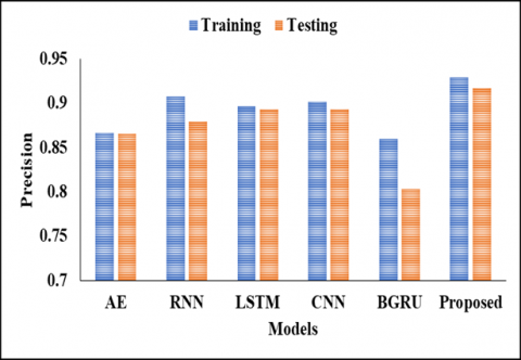
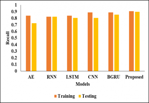
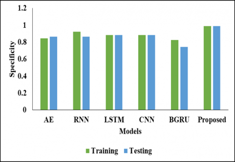
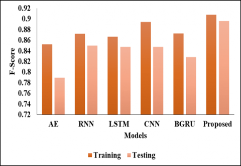
In Table 3 represent that the Comparative analysis on Training Values, in this analysis, the AE model reached the accuracy of 0.8407 and the precision value as 0.8667 and the recall value as 0.8387 and the specificity value of 0.8431 and another F1-Score value as 0.8525 and finally AUC score value as 0.9190 respectively. And RNN model reached the accuracy of 0.8673 0.9073 and the specificity value of 0.8226 and another F1-Score value as 0.9216 and finally the AUC value as 0.9219. Also, another type of LSTM model reached the accuracy of 0.8584 and the precision value as0.8929 and the recall value as 0.8966 and the recall value as 0.8387 and the specificity value of 0.8824 and another F1-Score value as 0.8667 and finally the AUC value as 0.9330 respectively. And another, CNN model reached the accuracy of 0.8850 and the precision value as 0.9016 and the recall value as 0.8871 and the specificity value of 0.8824 and another F1-Score value as 0.8943 0.9374 correspondingly. Next BGRU model reached the accuracy of 0.8584 and the precision value as 0.8594 and the recall value as 0.8871 and the specificity value of 0.8235 and another F1-Score value as 0.8730 and finally the AUC value as 0.9282 respectively. And finally, the proposed model reached the accuracy of 0.9818 and the precision value as 0.9293 and the recall value as 0.9082 and the specificity value of 0.9899 and another F1-Score value as 0.9081 and finally the AUC value as 0.9953 respectively. By this comparisons analysis, the proposed model reaches the better results than another compared model. This analysis is shown in Figures 2, 3, 4, 5 and 6.
Figure 1. Accuracy analysis
Table 2. Validation analysis on testing values
|
Models |
Accuracy |
Precision |
Recall |
Specificity |
F1 Score |
AUC Score |
|
AE |
0.7876 |
0.8654 |
0.7258 |
0.8627 |
0.7895 |
0.9089 |
|
RNN |
0.8407 |
0.8793 |
0.8226 |
0.8627 |
0.8500 |
0.9203 |
|
LSTM |
0.8407 |
0.8929 |
0.8065 |
0.8824 |
0.8475 |
0.9064 |
|
CNN |
0.8407 |
0.8929 |
0.8065 |
0.8824 |
0.8475 |
0.9089 |
|
BGRU |
0.8053 |
0.8030 |
0.8548 |
0.7451 |
0.8281 |
0.8786 |
|
Proposed |
0.9792 |
0.917 |
0.897 |
0.9884 |
0.8962 |
0.9944 |
Table 3. Comparative analysis on training values
|
Models |
Accuracy |
Precision |
Recall |
Specificity |
F1 Score |
AUC Score |
|
AE |
0.8407 |
0.8667 |
0.8387 |
0.8431 |
0.8525 |
0.9190 |
|
RNN |
0.8673 |
0.9073 |
0.8226 |
0.9216 |
0.8718 |
0.9219 |
|
LSTM |
0.8584 |
0.8966 |
0.8387 |
0.8824 |
0.8667 |
0.9330 |
|
CNN |
0.8850 |
0.9016 |
0.8871 |
0.8824 |
0.8943 |
0.9374 |
|
BGRU |
0.8584 |
0.8594 |
0.8871 |
0.8235 |
0.8730 |
0.9282 |
|
Proposed |
0.9818 |
0.9293 |
0.9082 |
0.9899 |
0.9081 |
0.9953 |
Figure 2. Validation analysis based on precision
Figure 3. Performance analysis
Figure 4. Specificity validation
Figure 5. Graphical representation in terms of F1-score
Figure 6. AUC analysis
Table 4. Performance analysis of proposed model
|
Methods |
Accuracy |
|
MLP |
87.5 |
|
AE |
90.1 |
|
RNN |
92.16 |
|
LSTM |
93.08 |
|
CNN |
94.7 |
|
BGRU |
95.0 |
|
Proposed |
98.18 |
In above Table 4 represent that the Performance analysis of proposed model. In this analysis, we used MLP model reached the accuracy score of 87.5 respectively. After the AE model reached the accuracy score of 90.1 respectively. Another RNN model reached the accuracy score of 92.16 respectively. In next LSTM model reached the accuracy score of 93.08 respectively. Afterward CNN model reached the accuracy score of 94.7 respectively. And then BGRU model reached the accuracy score of 95.0 respectively. And finally, the proposed model reached the accuracy score of 98.18 respectively. It is shown in Figure 7.
Figure 7. Validation analysis of proposed model in terms of accuracy
This paper introduces a unique CNN-BGRU-JBOA predictor model, which is used to estimate the charging needs for EV in the datasets under consideration. The proposed predictor model incorporated the strengths of various methods to improve prediction accuracy, including the empirical mode decomposition for lossless signal sub-series decomposition, the arithmetic optimisation algorithm for improved exploration and exploitation, the BGRU model with memory states for long-term memory retention, and deep learning for improved architecture layer depth and intensive training. The suggested predictor has been put through extensive simulation testing on the EV datasets, with results demonstrating its superiority over previously available prediction models for these data. Forecast accuracy of 98.18% with a very minimum MSE in the range of 10-10 demonstrates its efficacy, and training and testing efficiencies of the modelled predictor were assessed at 97 and 98, respectively, which is healthier than other state-of-the-art methodologies. With improved prediction accuracy and reduced error values, the CNN-BGRU-JBOA predictor has proven its worth in predicting the charging needs of EVs. The next study will involve giving the ideal features by employing optimisation models, as the irrelevant features may lead to low classification accuracy.
[1] Yi, Z., Liu, X. C., Wei, R., Chen, X., Dai, J. (2022). Electric vehicle charging demand forecasting using deep learning model. Journal of Intelligent Transportation Systems, 26(6): 690-703. https://doi.org/10.1080/15472450.2021.1966627
[2] Roy, A., Law, M. (2022). Examining spatial disparities in electric vehicle charging station placements using machine learning. Sustainable Cities and Society, 83: 103978. https://doi.org/10.1016/j.scs.2022.103978
[3] Ramineni, P., Pandian, A. (2021). Study and investigation of energy management techniques used in electric/hybrid electric vehicles. Journal Européen des Systèmes Automatisés, 54(4): 599-606. https://doi.org/10.18280/jesa.540409
[4] Ullah, I., Liu, K., Yamamoto, T., Shafiullah, M., Jamal, A. (2022). Grey wolf optimizer-based machine learning algorithm to predict electric vehicle charging duration time. Transportation Letters, 1-18. https://doi.org/10.1080/19427867.2022.2111902
[5] Li, Y., He, S., Li, Y., Ge, L., Lou, S., Zeng, Z. (2022). Probabilistic charging power forecast of EVCS: Reinforcement learning assisted deep learning approach. IEEE Transactions on Intelligent Vehicles, 8(1): 344-357. https://doi.org/10.1109/TIV.2022.3168577
[6] Inamanamelluri, H.V.S.L., Pulipati, V.R., Pradhan, N.C., Chintamaneni, P., Manur, M., Vatambeti, R. (2023). Classification of a new-born infant’s jaundice symptoms using a binary spring search algorithm with machine learning. Revue d'Intelligence Artificielle, 37(2): 257-265. https://doi.org/10.18280/ria.370202
[7] Ma, T.Y., Faye, S. (2022). Multistep electric vehicle charging station occupancy prediction using hybrid LSTM neural networks. Energy, 244: 123217. https://doi.org/10.1016/j.energy.2022.123217
[8] Shanmuganathan, J., Victoire, A.A., Balraj, G., Victoire, A. (2022). Deep learning LSTM recurrent neural network model for prediction of electric vehicle charging demand. Sustainability, 14(16): 10207. https://doi.org/10.3390/su141610207
[9] Boulakhbar, M., Farag, M., Benabdelaziz, K., Kousksou, T., Zazi, M. (2022). A deep learning approach for prediction of electrical vehicle charging stations power demand in regulated electricity markets: The case of Morocco. Cleaner Energy Systems, 3: 100039. https://doi.org/10.1016/j.cles.2022.100039
[10] Eddine, M.D., Shen, Y. (2022). A deep learning based approach for predicting the demand of electric vehicle charge. The Journal of Supercomputing, 78(12): 14072-14095. https://doi.org/10.1007/s11227-022-04428-0
[11] Devendran, M., Rajendran, I., Ponnusamy, V., Marur, D.R. (2021). Optimization of the convolution operation to accelerate deep neural networks in FPGA. Revue d'Intelligence Artificielle, 35(6): 511-517. https://doi.org/10.18280/ria.350610
[12] Zhao, D., Wang, H., Liu, Z. (2022). Charging-related state prediction for electric vehicles using the deep learning model. Journal of Advanced Transportation, 2022. https://doi.org/10.1155/2022/4372168
[13] Suriya, N., Vijay Shankar, S. (2022). A novel ensembling of deep learning based intrusion detection system and scroll chaotic countermeasures for electric vehicle charging System. Journal of Intelligent & Fuzzy Systems, 43(4): 4789-4801. https://doi.org/10.3233/JIFS-220310
[14] Aljafari, B., Jeyaraj, P.R., Kathiresan, A.C., Thanikanti, S.B. (2023). Electric vehicle optimum charging-discharging scheduling with dynamic pricing employing multi agent deep neural network. Computers and Electrical Engineering, 105: 108555. https://doi.org/10.1016/j.compeleceng.2022.108555
[15] Luo, S.Y., Gu, Y.J., Yao, X.X., Fan, W. (2021). Research on text sentiment analysis based on neural network and ensemble learning. Revue d'Intelligence Artificielle, 35(1): 63-70. https://doi.org/10.18280/ria.350107
[16] Mazhar, T., Asif, R.N., Malik, M.A., Nadeem, M.A., Haq, I., Iqbal, M., Kamran, M., Ashraf, S. (2023). Electric vehicle charging system in the smart grid using different machine learning methods. Sustainability, 15(3): 2603. https://doi.org/10.3390/su15032603
[17] Venkitaraman, A.K., Kosuru, V.S.R. (2023). Hybrid deep learning mechanism for charging control and management of electric vehicles. European Journal of Electrical Engineering and Computer Science, 7(1): 38-46. http://dx.doi.org/10.24018/ejece.2023.7.1.485
[18] Hafeez, A., Alammari, R., Iqbal, A. (2023). Utilization of EV charging station in demand side management using deep learning method. IEEE Access, 11: 8747-8760. https://doi.org/10.1109/ACCESS.2023.3238667
[19] Aduama, P., Zhang, Z., Al-Sumaiti, A.S. (2023). Multi-feature data fusion-based load forecasting of electric vehicle charging stations using a deep learning model. Energies, 16(3): 1309. https://doi.org/10.3390/en16031309
[20] Kotapati, G., Ali, M.A., Vatambeti, R. (2023). Deep learning-enhanced hybrid fruit fly optimization for intelligent traffic control in smart urban communities. Mechatronics and Intelligent Transportation Systems, 2(2): 89-101. https://doi.org/10.56578/mits020204
[21] Luo, R., Song, Y., Huang, L., Zhang, Y., Su, R. (2023). AST-GIN: Attribute-augmented spatiotemporal graph informer network for electric vehicle charging station availability forecasting. Sensors, 23(4): 1975. https://doi.org/10.3390/s23041975
[22] Mohammed, H., Tannouche, A., Ounejjar, Y. (2022). Weed detection in pea cultivation with the faster RCNN ResNet 50 convolutional neural network. Revue d'Intelligence Artificielle, 36(1): 13-18. https://doi.org/10.18280/ria.360102