Souad Abbas![]() | Hamouma Moumen
| Hamouma Moumen![]() | Fayçal Abbas*
| Fayçal Abbas*![]()
© 2023 IIETA. This article is published by IIETA and is licensed under the CC BY 4.0 license (http://creativecommons.org/licenses/by/4.0/).
OPEN ACCESS
One of the main ways of economic development has been to improve the performance and efficiency of manufacturing systems. Indeed, competition is fierce between most industrial organizations to provide new products and richer services for customers who are increasingly demanding. Although, indeed, most of the quality control and visual inspection tasks are performed by humans who use only the naked eye to detect defects, this form of control presents a number of limits, such as the size of the defects impossible to detect, risk of marketing a defective product and reduce the production performance. In this paper, a new method based on deep learning in the context of ceramic tile defect detection on a conveyor is proposed in order to provide effective quality control and real-time inspection. Our model is based on a convolutional architecture with a convolutional block attention module (CBAM) to pay more attention to the relevant areas of the input image and overcome the spatial information loss problems. A pre-processing step is performed before training by processing each image corresponding to a type of defect with an appropriate mask to facilitate learning. The experimental results show that our model produces an accurate and efficient classification of ceramic tile defects with a reduced number of parameters. We also propose a novel Ceramic defect tile dataset obtained from a ceramic production unit. The results of the experiments show that the suggested approach reaches an average accuracy rate of 99.93% compared to the state-of-the-art.
defect detection, convolutional neural network, attention mechanism, CBAM
Ensuring effective visual inspection is increasingly becoming a complex task for many industrial companies. With the evolution of artificial intelligence, it seems essential to take advantage of this progress to provide machine vision solutions based on deep learning approaches for visual inspection, quality control, and object recognition in an industrial context.
The task of detecting defects in ceramic tiles in the industry is a complex task. The latter is due to the diversity in the shape, appearance, and number of tiles to be treated in this way in most production units average, this task is performed by a human. Manual surface quality inspection represents a significant challenge to maintain customer satisfaction since it is tedious, repetitive for humans, and performed in an environment with noise, extreme temperature, and humidity [1], making detecting faults easy.
During the production stages of ceramic tiles, different defects affect the quality of tile surfaces, such as cracks, spots, pinholes, and corner or edge breaks. Thus for complete automation of the ceramic tile quality inspection system, other problems have to be solved, especially the diversity of defects in terms of shape and texture.
Indeed, different solutions have been presented in the literature to address the limitations of manual detection of surface defects. However, the traditional techniques are characterized by the lack of robustness of the proposed systems and reduced production performances.
Recent techniques based on convolutional neural networks have appeared. These offer automatic feature extraction using different filters on a 2D image. However, convolutional neural networks lose spatial information, which prevents efficient local and global feature extraction to remedy this problem in the context of ceramic tile defect detection. Our idea is to integrate a CBAM attention module in a convolutional neural network to pay more attention to the relevant areas of the input image. Thus, increase the number of instances by generating a mask image for all samples of the default class for each image. This step allows the neural network to easily recognize the patterns' positions in the input image and facilitate learning. The surface defects taken into account by our model are corner breaks, pinholes, and pattern discontinuity.
In this paper, the main contributions are summarized as follows:
(1) We propose a new method based on convolutional neural networks with CBAM attention mechanism to have local and global feature extraction, allowing the CNN to focus on relevant pixels and provide an efficient classification of ceramic tile defects.
(2) We introduce a new dataset of real images for ceramic tile defect detection. Our dataset considers three types of defects (corner breaks, pinholes, and pattern discontinuity).
(3) The efficiency of the pre-processing part is proved through a quantitative comparison and the integration of the attention module is validated through an ablation study.
Traditional defect detection algorithms have not achieved stable results despite a strong dependence on illumination, disk grain structure, defect morphology, and defect size [2]. On the other hand, several studies have been presented to achieve high accuracy for defect detection on ceramic tiles [3-9]. Ragab and Alsharay [3] have proposed a solution consisting of two steps to minimize the time required for detecting defects in ceramic images. In the first step, it detects defects in each of the eight parts of the image, and in the second, it determines their type using the algorithms of defects of spots and cracks. experiments show that the time of detection and classification of defects in ceramic tiles is reduced compared to previous work. However, they are used a limited number of images and it is limited to too low detection rate. Hanzaei et al. [4] used processing techniques such as median filter, local variance rotation invariant measure, thresholding, and morphological closure operations, and then use a support vector machine (SVM) for multiclass classification. This solution improves the automatic detection rate of cracks and holes on ceramic tile surfaces by accurately detecting edge and defect regions and eliminating unimportant areas. However, this work does not deal with tile’s textured surfaces. While Chen et al. [5] used a decision tree algorithm to classify the defects of textured ceramic tiles based on a Fourier transformer to remove the background, they applied Laplacian sharpening, histogram specification, and median filtering. They then extracted the features using Lavel Co-occurrence Matrix (GLCM) and Casagrande et al. [6] proposed a hybrid algorithm to extract features from smooth and textured ceramic tile images, a combination of segmentation-based fractal texture analysis and discrete wavelet transform methods was used after applying the preprocessing techniques, which were then introduced for the five classifiers. Within them, the SVM classifier reaches 99.01% for smooth images and 97.89% for textured images. This solution only deals with the defects of the pattern's discontinuity despite using textured tiles. In addition, it is limited to a single model of the pattern of textured ceramic tiles. Mariyadi et al. [7] proposed to use GLCM to extract fourteen properties of the defect area, which are then sent to the artificial neural network for classification. The defect area was clipped from the image after counting the mean hue, deviation square and euclidean distance, threshold segmentation, and morphological operation. Despite the limited number of images without texture, there are errors in the classification of defects, especially the pinholes which classify as crack. Zorić et al. [8] developed a method for detecting defects on the surfaces of biscuit tiles which based on Fourier Spectrum for extraction features of defects and on K-nearest neighbors (KNN) and random forest for classification. Zhang et al. [9] proposed an efficient method is proposed based on three basic steps: image preprocessing, defect detection, and defect determination. The authors remove the background information by SRR algorithm, adjust the lateral contrast, and then apply the spatial distribution variance (CSDA) and the color spot area weight (CSAW) to the HSV color. A defect saliency map is generated, and the defect area is divided into blocks according to the boundaries of the defect rectangle to extract the feature vector color, which is then fed to the SVM algorithm. The method achieves good performance with an accuracy rate of 98.75%. The performance of this method decreases with the increase in the complexity and variety of the textures of the tile surfaces, due to the increase in the number of characteristics of the colors to be represented.
However, recent contributions based on deep learning models have appeared. A new method, "Segmentation Model for Cracks in Ceramics (CCS)," is proposed [10]. Indeed, the latter is based on the U-net model and a combination of pre-processing techniques that are applied to the images to render prominent cracks in a white and perfect font based on morphological and correction operations. The accuracy of defect detection is very high, reaching 99.9%. However, the effectiveness of this solution has been tested on a limited number of ceramic tile images and does not treat just one defect. Nogay et al. [11] used the AlexNet pre-trained model to classify invisible cracks in ceramic tile images based on acoustic noise. Indeed, a dataset of nine classes of invisible crack images of different sizes but similar structural properties are introduced. The model achieves better accuracy in detecting cracks. The model achieves better accuracy in detecting cracks despite the generalization supported by this work. However, it does not specify the location of cracks, which is essential for automated inspection of cracks, and it does not remove noise in images. Thus, a limited number of images are used for training and testing. While Stephen et al. [12] proposed a lightweight convolutional neural network to automate the detection of cracks in ceramic tiles with smooth surfaces. Feature extraction and classification are performed in parallel in this CNN model. Indeed a better accuracy in detecting cracks is obtained.
3.1 Convolutional block attention module (CBAM)
The attention mechanism has significantly improved the performance of defect inspection applications in several areas: agriculture [13, 14], medical [15, 16] and industrial [17, 18], because of its ability to mimic human perception to focus on salient regions and neglect that are not important. For example, among the intention modules used to increase the performance of detection of defects in industrial products are various that easily integrate with convolutional neural networks such as Convolutional Block Attention Module (CBAM) [19], Squeeze-and-Excitation Attention Module (SE) [20], Dual attention Module (DAM) [21] and Bottleneck Attention Module (BAM) [22].
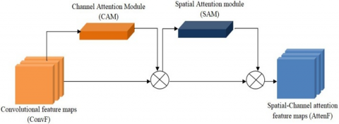
CBAM is one of the usable intent modules that help pay more attention to relevant areas of the image. It consists of two attention modules to allow the network to extract the relevant features by focusing on what to pay attention by the Channel module and where to pay attention by the Spatial module. The overall architecture of the CBAM module is shown in Figure 1.
The general function of CBAM, as shown in Eq. (1), is to generate an attentional feature map (AttenF) from a convolutional feature map (ConvF) accepted as input that will be multiplied with the Channel feature map and a Spatial feature map.
AttenF=SAM(CAM(ConvF)ConvF). (CAM(ConvF)×ConvF) (1)
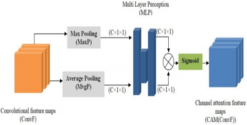
CAM(ConvF) represents the channel feature map generated by the Channel Attention Module (CAM), which is described in Figure 2. CAM consists of a Max Pooling (MaxP) and Average Pooling (AvgP) layer in parallel. Then, the multilayer perceptron (MLP) and a sigmoid function are applied. Mathematically, this map is formulated by the following formula:
CAM(ConvF)=sigmoid(MLP(AvgP(ConvF)+MLP(MaxP(ConvF)))) (2)
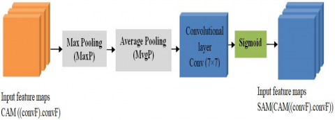
SAM(CAM(ConvF)ConvF) represents the spatial feature map generated by the Spatial Attention Module (SAM), whose architecture is illustrated in Figure 3. SAM sequentially contains a max pooling layer and an average pooling layer, followed by a single convolutional layer of size 7×7 (Convf) and a sigmoid function, as shown in the following equation:
$\operatorname{SAM}(\operatorname{CAM}(\operatorname{ConvF}) \operatorname{ConvF})=\operatorname{sigmoid}\left(\operatorname{Convf}^{7 \times 7}\left(\left[\begin{array}{l}\operatorname{Avg} P(\operatorname{CAM}(\operatorname{ConvF}) \operatorname{ConvF}) ; \\ \operatorname{MaxP}(\operatorname{CAM}(\operatorname{ConvF}) \operatorname{ConvF})\end{array}\right]\right)\right)$ (3)
Figure 1. Architecture of the CBAM attention module
Figure 2. Architecture of the Channel Attention Module (CAM)
Figure 3. Architecture of the Spatiale Attention Module (SAM)
This section presents the steps corresponding to our solution and the proposed architecture to improve the detection of ceramic tile defects.
4.1 An overview of the solution proposed
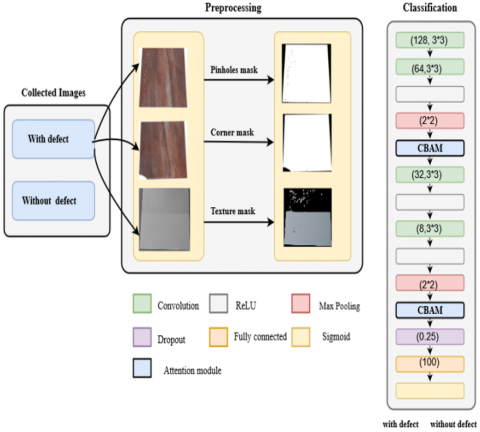
In this paper, a new model based on convolutional architecture is proposed to improve the detection of defects in ceramic tiles. Our solution operates in three main steps, which are; data collection, preprocessing, and classification. Indeed, the collection step consists in collecting images of ceramic tiles with and without defects. The second step consists of a preprocessing of the collected images, allowing the treatments carried out in this step to remove the background and the generation of the mask for the images with a defect. The last step is to classify ceramic tiles using a convolutional neural network, and in order to increase the efficiency and performance of our model of classification of defects for ceramic tiles, we have introduced two layers of attention in our CNN. The latter takes RGB images as input and produces a binary classification with defect or without defect. Figure 4 shows the global architecture of the proposed solution.
Figure 4. The global architecture of our solution
4.2 Collected images
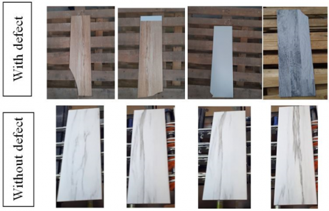
We introduce a new dataset for defect detection of ceramic tiles. The collected images are 1032 RGB images. These images are of different shapes (rectangular and square) and appearances (texture, illumination). The collected images are divided into two classes defect and no defect. Figure 5 below shows samples of the collected defect-free and defect images.
Figure 5. Examples of images from our dataset
4.3 Preprocessing
The preprocessing step of our model consists of two phases. The first is to remove the background from the image, and the second phase is to create a mask for the defective images to better represent the position and shape of the defects and reduce the complexity of detecting it on the ceramic tiles. In the automation of the industrial inspection system, the great challenge is detecting the different types of defects in the texture surfaces [23]. Indeed, the specificity of each defect on a ceramic requires a different treatment for the creation of the mask. The purpose of adding these masks is to improve the representation of features. In our solution, we have adopted three types of masks for the images of the defective tiles: the first two are highlighted the breaks of the corners of the ceramic tiles and the pinholes via the segmentation and morphological operations. Thus, one extracts the white parts, which appeared because of the discontinuity of the textures.
4.3.1 Corner and pinholes masks
This step consists in creating a binarized image, where the pixels of the latter are composed of two black and white values. Then, from a grayscale image, we use the Otsu function [24] with the operation of inversion to identify the tile in white and the background and the pinholes in black. The Otsu method created by Nobuyuki Otsu which is an automatic thresholding method that is based on the search in the histogram of the image on the optimal value among the thresholding values denoted (t) which is in the interval [0, 255]. Indeed, this is calculated with maximize the variance inter-classes, denoted by $\left(\sigma_y^2\right)$ and minimize the variance intra-classes denoted by $\left(\sigma_w^2\right)$ for separate the pixel values of the background (bg) and foreground (fg). These are calculated by following equations:
$\sigma_w^2(t)=\omega_{b g}(t) \sigma_{b g}^2(t)+\omega_{f g}(t) \sigma_{f g}^2(t)$ (4)
$\sigma_y^2=\sigma^2-\sigma_w^2$ (5)
$\omega_{b g}=\sum_{i=0}^t P(i)$ (6)
$\omega_{f g}=\sum_{i=t+1}^{255} P(i)$ (7)
Such as:
ωbg: presents the sum of the probabilities of the pixels P(i) which are lower than the threshold t devised by the overall probability of all pixels of an image.
ωfg: presents the sum of the probabilities of the pixels P(i) greater than the threshold t divided by the overall probability of all an image's pixels.
where: the probability of pixels is calculated by this equation:
$P(i)=\frac{n_i}{n}$ (8)
ni: the value of the ieme pixelin image.
n: the average value of all pixels of the background and foreground classes.
$\sigma_{\mathrm{bg}}^2$: presents the variance of background class and $\sigma_{\mathrm{fg}}^2$: presents the variance of foreground class, where are calculated:
$\sigma_{b g}^2=\frac{\sum_{i=0}^t \, \, \left(N 1(i)-M o y_{b g} \, (T)\right) \, \, ^2 \, \, \times P(i)}{\omega_{b g}}$ (9)
$\sigma_{b f}^2=\frac{\sum_{i=t+1}^{255} \, \, \, \, \left(N 2(i)-M o y_{b f}(T)\right) \, \, ^2 \, \, \times P(i)}{\omega_{b f}}$ (10)
where:
N1: is a vector from 0 to t-1.
N2: is a vector from t to 255.
Moybg: the average of the background class and Moyfg: the average of the foreground class, which are calculated by the following equations:
$\operatorname{Moy}_{b g}(t)=\frac{\sum_{i=0}^t \, \, \, \, N 1(i) \times P(i)}{\omega_{b g} \,(t)}$ (11)
$\operatorname{Moy}_{f g}(t)=\frac{\sum_{i=t+1}^{255} \, \, \, \, N 2(i) \times P(i)}{\omega_{f g} \, (t)}$ (12)
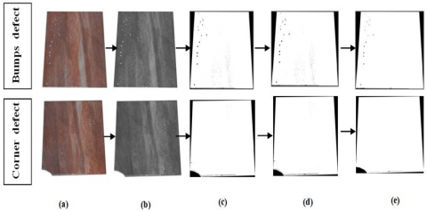
Finally, we remove the noise from the binary images by operating the morphological opening with a filter of a size 3×3 filled by ones to obtain a clear image, followed by a dilation operation. Figure 6 shows a resulting pinholes and corner mask after performing this series of operations on two faulty images.
Figure 6. The steps to generate a mask of two images with a default: (a) Input image, (b) Gray scale, (c) Binary image, (d) Opening morphology and (e) Mask image
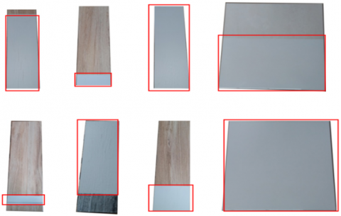
Figure 7. Defective images with the locations of the pattern discontinuity by red rectangles
4.3.2 Texture mask
In order to obtain a more precise representation of the discontinuity of patterns on the surfaces of ceramic tiles like the examples shown in Figure 7, we used the HSV (Hue Saturation Value) color mode [25], which Alvy Ray Smith creates. This model is a system of human visual perception consisting of three components: Hue (color), Saturation (intensity), and Value (brightness). Studies use the HSV color mode to improve color defects in colored images, such as detecting defects in fruit [26] and on the surface of printing rollers [27].
For conversion between RGB mode to HSV mode, the three values: Red (R), Green (G), and Blue (B), are used to calculate the H, S, and V values according to the following functions knowing that: $R, G, B \in[0,1]$.
$M a x=\max (R, G, B)$ (13)
$\operatorname{Min}=\min (R, G, B)$ (14)
$H=\left\{\begin{array}{l}0, \text { if } R=G=B \\ 60^{\circ} \times\left(0+\frac{G-B}{\text { Max-Min }}\right), \text { if Max }=R \\ 60^{\circ} \times\left(2+\frac{B-R}{\text { Max-Min }}\right), \text { if Max }=G \\ 60^{\circ} \times\left(4+\frac{R-G}{\text { Max-Min }}\right), \text { if Max }=B\end{array}\right.$ (15)
$S= \begin{cases}0, & \text { if } R=G=B \\ \frac{\text { Max-Min }}{\text { Max }}, & \text { else }\end{cases}$ (16)
V=Max (17)
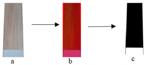
An example of the texture mask is shown in Figure 8.
Figure 8. Generation of a texture mask (c) from the input image (a) HSV mode (b)
4.4 Classification
Our ceramic tile classification model has an architecture that combines a convolutional neural network (CNN) and an attention mechanism. The CNN is composed of four convolutional layers, two first consequential layers to extract the low level characteristics, followed by a ReLU activation function and a Maxpooling layer. Then the CBAM layer followed by two convolutional layers. After each layer a ReLU function is applied. The second CBAM attention module is inserted. We adopted a regularization using the dropout by a factor of 0.25 to avoid overfitting. Finally, a fully connected (FC) layer with 100 neurons followed by a sigmoid activation function to classify the input image whose dimension is 210×210×3 as defective or not.
5.1 Dataset and data augmentation
Our dataset comprises two labels, defect, and non-defect, for binary classification. The defect class comprises the images of the three defects considered in our study. A data augmentation operation is applied to increase the number of samples in the training data and reduce the risk of overfitting. For the faulty tile images, we applied 180 degree rotation method, horizontal and vertical flip, zoom, and shear techniques with 20% range. At the same time, we applied 2 degree rotation only for normal images to maintain the correct shape of the tiles and avoid breakage. Table 1 describes the total number of images before and after augmentation for the images.
Indeed, after the preprocessing step, which consists in adding the default image masks. We have created three distributions of images from the dataset to perform our experiments to evaluate the performance of our model. The details of the distributions are shown in Table 2. Dataset 1 is used for binary classification, dataset 2 is used for multiclass classification and dataset 3 is composed of images without masks.
Table 1. The numbers of the images before and after the increase
|
|
Classes |
Before augmentation |
After augmentation |
Total images |
|
Defects |
Corners |
102 |
1020 |
1122 |
|
Pinholes |
143 |
1110 |
1253 |
|
|
Pattern discontinuity |
117 |
1096 |
1275 |
|
|
|
No defects |
670 |
438 |
1108 |
Table 2. Description of the datasets of the images of the ceramic tiles
|
Datasets |
Classes |
Training set |
Validation set |
||
|
Image |
Mask |
Image |
Mask |
||
|
Dataset 1 |
Defect |
2538 |
2538 |
636 |
636 |
|
No defect |
212 |
/ |
212 |
/ |
|
|
Dataset 2 |
Corners |
846 |
846 |
212 |
212 |
|
Pinholes |
846 |
846 |
212 |
212 |
|
|
Pattern discontinuity |
846 |
846 |
212 |
212 |
|
|
No defect |
846 |
/ |
212 |
/ |
|
|
Dataset 3 |
Defect |
2538 |
/ |
636 |
/ |
|
No defect |
212 |
/ |
212 |
/ |
|
5.2 Training details and evaluation metrics
The set of images in our dataset is divided into 80% for training and 20% for validation. The learning rate is 1e-3, we used the RMSprop optimizer, the batch size is 15, the input image size is set to 120×120, and the experiments are performed on a machine with an Intel Core i5-10400F processor and an Nvidia GTX 1050ti GPU. In order to show the effectiveness of our model, we choose accuracy, precision, and recall as metrics to evaluate the performance. These are calculated from the confusion matrix values, as presented in Table 3.
Table 3. Values of the confusion matrix
|
True label |
Predicted label |
|
|
TP |
FP |
|
|
FN |
TN |
|
TP and TN exhibit tiles that are correctly predicted as defective and non-defective, respectively. FN presents those that are non-defective, but the model predicted them to be defective. In contrast, FP defines defective tiles that are identified as non-defective. The following equations define the three metrics:
Accuracy $=\frac{T P+T N}{T P+T N+F P+F N}$ (18)
Precision $=\frac{T P}{T P+F P}$ (19)
Recall $=\frac{T P}{T P+F N}$ (20)
Accuracy presents the number of tiles correctly predicted out of the total number. Accuracy presents the number of tiles correctly predicted as faults out of the total number of faulty tiles revealed. Finally, the recall presents the number of tiles that correctly predicted defects out of the total number predicted as defective.
In this section, we present the results obtained by our model. Indeed, an evaluation of the effect of the parameters chosen for our model, a quantitative comparison with state-of-the-art methods, and finally, an ablation study is conducted to show the efficiency of each component of our model.
6.1 Performance evaluation of setting parameters of CBAM module
For the CBAM attention module, we tested the performance of the variant configurations for more efficiency in detecting faults. In fact, experiments are menu by varying the values of the reduction ratio of the channel module.
6.1.1 The Ratio reduction (R)
Table 4 presents the results of experiments comparing the accuracy, precision, and recall of the classification obtained by our model with the values 8, 16, and 32 assigned to the ratio of the channel module reduction. In this study, we have kept the default filter size of the convolutional layer of the spatial module, which is 7.
All accuracies achieved by the three combinations are satisfactory. Perfect accuracy is reached by minimizing the dimensions of the feature maps by the ratio 16, while for the values 32 and 8, a decrease in the accuracy is observed by 0.07% and 0.14%, respectively. Indeed, the exact choice of the ratio considerably improves the relevant features generated in the channel attention maps. Consequently, better performances of defects detection are achieved.
Table 4. Comparison of classification accuracies according to Channel module reduction ration values
|
Models |
Accuracy (%) |
Precision (%) |
Recall (%) |
|
Our CNN+Channel (R=8) |
99.79 |
99.84 |
99.92 |
|
Our CNN+Channel (R=16) |
99.93 |
100 |
99.92 |
|
Our CNN+Channel (R=32) |
99.86 |
99.84 |
100 |
6.1.2 The impact of the number and position of CBAM module
Table 5 illustrates the performance evaluation of our model as a function of the position and number of the CBAM module in our CNN model. Indeed, a variation of accuracy, precision, and recall are analyzed to choose the optimal configuration to obtain an efficient extraction of discriminative features.
We note from the results shown in Table 5 that the integration of the two CBAM modules after the conv 2 and conv 4 layers, respectively, produces good defect classification performance in terms of accuracy of 99.93%, precision of 100%, and recall of 99.92%. In addition, the extraction of relevant features after conv1 by the CBAM module leads to a significant classification of defects by an accuracy of 99.86%, precision of 99.92%, recall of 99.92%.
Table 5. The effect of position and number of the CBAM attention module on the performance of our model
|
Position of CBAM |
Accuracy (%) |
Precision (%) |
Recall (%) |
|
After Conv 1 |
99.86 |
99.92 |
99.92 |
|
After Conv 2 |
98.64 |
98.27 |
99.44 |
|
After Conv 3 |
99.46 |
99.60 |
99.76 |
|
After Conv 4 |
99.59 |
99.68 |
99.84 |
|
After Conv 2 + after conv 4 (Our model) |
99.93 |
100 |
99.92 |
In this section, we will discuss the choice of parameters of our proposed model to effectively classify tile images, including the learning rate and classification type.
6.1.3 The impact of learning rate values
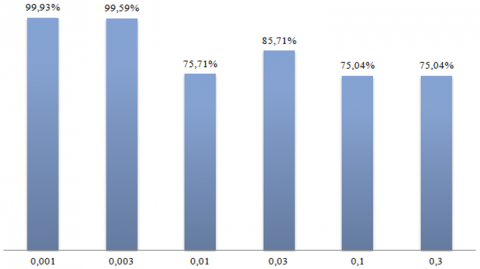
Figure 9. The effect of learning rate on the classification accuracy of our CNN model
Figure 9 shows the accuracy of the validation for various learning rates. The validation accuracy decreases when the learning rate is too high 0.01. When the learning rate is 0.01, the best performance is attained. The accuracy value reaches 99.93%.
6.1.4 Effect of type of classification
Table 6 shows the effect of the type of classification (binary or multiclass) on the performance of our model in classifying the images of ceramic tiles. Indeed, we used two datasets to prove the efficiency of our model. Dataset 1 is a binary dataset where the tiles are organized in two classes, defect, and non defect, while dataset 2 is a multiclass dataset where the images of the non defect class are divided into three distributions corresponding to the three types of defects taken into consideration by our study: with corner breakage, pinholes, and pattern discontinuity.
The three evaluation metrics, accuracy, precision, and recall, are used to measure the performance of our model for a binary classification on dataset 1 and multiclass on dataset 2.
Table 6 illustrates the comparison results among binary classification and multi-classification tasks. These results demonstrated a significant distinction between our model's binary and multiclass classification. Compared to a multiclass classification, where each type of defect is represented by a different class, our model generalizes more effectively for the binary classification of ceramic tiles. Our model performs better with a binary classification, increasing accuracy, precision, and recall by 4.18%, 4.09%, and 0.82% respectively.
Table 6. Classification performance of our model on different datasets
|
Datasets |
Accuracy (%) |
Precision (%) |
Recall (%) |
|
Dataset 1 |
99.93 |
100 |
99.92 |
|
Dataset 2 |
95.75 |
95.91 |
99.10 |
6.2 Effect of masks
Augmenting our dataset with mask images in the preprocessing part plays a significant role in improving the performance of our solution. Indeed, to evaluate the effect of adding the masks to the defect images on the performance of tile defect classification, we compare performances of our model on dataset 1 and dataset 3.
Table 7. Performance comparison results of our model on dataset 1 and dataset 3
|
Datasets |
Accuracy (%) |
Precision (%) |
Recall (%) |
|
Dataset 1 |
99.93 |
100 |
99.92 |
|
Dataset 3 |
97.30 |
97.56 |
99.20 |
From the results presented in Table 7, the masks added to the defect images in dataset 1 significantly affect our CNN model's performance of ceramic tile defect classification. Without the masks, the defect detection accuracy decreases to 97.30%, with a precision of 97.56% and recall of 99.20%. However, with the addition of the masks of the defect images based on segmentation and morphological operations and HSV color mode, a performance improvement is achieved by 2.63% and 2.44% for accuracy and precision, respectively.
6.3 Quantitative comparison
In this section, we compare the performance of our model with existing state-of-the-art methods: VGG16-19 [28], AlexNet [29], and ResNet50 [30]. The training of these models on the dataset takes place with the same hyper-parameters mentioned in the previous section. We used two scores: the overall accuracy of classification and the number of network parameters. The results obtained after training these models on our dataset composed of two classes with defects and without defects are presented in Table 8. We observe that our model, based on a convolutional architecture and integrating a CBAM attention module, outperforms the four models in terms of accuracy. Furthermore, our model produces good results with a significantly reduced number of parameters compared to existing models.
Table 8. Quantitative comparison between our model and the state of the art methods
|
Models |
Accuracy (%) |
Trainable parameters |
|
VGG 16 |
85.04 |
107,001,665 |
|
VGG 19 |
85.00 |
112,311,361 |
|
AlexNet |
93.02 |
29,972,545 |
|
ResNet 50 |
98.18 |
23,536,577 |
|
Our model |
99.93 |
2,346,337 |
6.4 Ablation study
We conducted an ablation study to show the effectiveness of the attention module in our architecture.
In this experiment, we investigated the CBAM attention module's effect on ceramic tiles' defect classification results. Table 9 compares our CNN architecture without CBAM attention module integration which noted CNN_base and our proposed model with CBAM attention module integration.
Table 9. Ablation study results of the CBAM module on the classification performance of our model
|
Models |
Accuracy (%) |
Precision (%) |
Recall (%) |
|
CNN_base |
98.98 |
99.84 |
99.37 |
|
Our model |
99.93 |
100 |
99.92 |
These results show that our model based on the CBAM module produces good results compared to the basic model in terms of accuracy, precision, and recall. Indeed, integrating the CBAM module provides more efficiency and precision to the tile classification results on our dataset. Furthermore, these results show that the CBAM attention module allows us to focus on the ceramic tiles' relevant features to localize the defects, which allowed us to increase the performance of our model.
In this paper, we proposed a model based on convolutional neural networks and the attention mechanism to detect defects in ceramic tiles more efficiently. The results show that our model performs better classification of different types of defects. Furthermore, the accuracy of defect classification by our model for binary classification outperforms most of the proposed state-of-the-art models, including models based on segmentation methods and feature extraction methods with machine learning algorithms [6-9] and models based on deep learning [11, 12]. This is related to the efficiency and robustness of the proposed preprocessing and classification step. Indeed, on the one hand, the increase in defective images is represented by the addition of masks that improve the visual representation of defects. On the other hand, the integration of the CBAM attention module. Moreover, our model reduces the computation cost thanks to the reduced number of parameters. On the other hand, the proposed model to automate the defect detection of ceramic tiles suffers from some limitations, a decrease in the defect detection rate for multi-class classification.
The accurate detection of defects in ceramic tiles, until now, is a significant issue for researchers due to the difficulty of distinguishing between defects and surface texture. Therefore, in this paper, to address this challenge, we propose a solution for accurate defect detection of ceramic tiles based on deep learning and attention mechanism.
Our solution consists of three fundamental steps: the first step consists in collecting real images from a production unit, preprocessing, and classification.
Our model is capable of classifying with high precision the three defects (corner breaks, pinholes, and pattern discontinuity) through a binary classifier based on the convolutional architecture equipped with a CBAM attention module. Furthermore, given the complexity imposed by the defects of the ceramic tiles and to simplify the learning of the ceramic defects, a preprocessing step is carried out on the images of the data set by applying several masks according to each defect in order to expose the characteristics of defects better, this simplifies learning and improves the performance of classifying ceramic tile defects.
Integrating the CBAM module into our CNN model allows our model to extract the local and global characteristics of defects, which greatly improves the performance of our model and produces good results compared to state-of-the-art methods.
As future work, we want to integrate our model into an industrial vision system capable of providing all the essential information concerning the defects of the ceramic tiles to the control room. Indeed we plan to improve our model to offer a muti-class classification that includes more defects and exact identification of the ceramic tiles by using RFID tags attached to the ceramic tiles to send the classification result to the processing center via a Zigbee protocol.
The authors would like to thank the Ceramics & Sanitary Tiles production company, TECHNOCERAM, for its support in collecting the images for this study.
[1] Elbehiery, H., Hefnawy, A., Elewa, M. (2007). Surface defects detection for ceramic tiles using image processing and morphological techniques. International Journal of Computer and Information Engineering, 1(5): 1488-1492. https://doi.org/10.5281/zenodo.1084534
[2] Havryliv, D., Ivakhiv, O., Semenchenko, M. (2020). Defect detection on the surface of the technical ceramics using image processing and deep learning algorithms. In 2020 21st International Conference on Research and Education in Mechatronics (REM), Cracow, Poland, IEEE, pp. 1-3. https://doi.org/10.1109/REM49740.2020.9313910
[3] Ragab, K., Alsharay, N. (2017). An efficient defect classification algorithm for ceramic tiles. Advanced Topics in Intelligent Information and Database Systems, 9: 235-247. https://doi.org/10.1007/978-3-319-56660-3
[4] Hanzaei, S.H., Afshar, A., Barazandeh, F. (2016). Automatic detection and classification of the ceramic tiles’ surface defects. Pattern Recognition, 66: 174-189. https://doi.org/10.1016/j.patcog.2016.11.021
[5] Chen, S., Lin, B., Han, X., Liang, X. (2013). Automated inspection of engineering ceramic grinding surface damage based on image recognition. The International Journal of Advanced Manufacturing Technology, 66: 431-443. https://doi.org/10.1007/s00170-012-4338-2
[6] Casagrande, L., Macarini, L.A.B., Bitencourt, D., Fröhlich, A.A., de Araujo, G. M. (2020). A new feature extraction process based on SFTA and DWT to enhance classification of ceramic tiles quality. Machine Vision and Applications, 31(7): 1-15. https://doi.org/10.1007/s00138-020-01121-1
[7] Mariyadi, B., Fitriyani, N., Sahroni, T.R. (2021). 2D detection model of defect on the surface of ceramic tile by an artificial neural network. Journal of Physics: Conference Series, 1764(1): 012176. IOP Publishing. https://doi.org/10.1088/1742-6596/1764/1/012176
[8] Zorić, B., Matić, T., Hocenski, Ž. (2022). Classification of biscuit tiles for defect detection using Fourier transform features. ISA Transactions, 125: 400-414. https://doi.org/10.1016/j.isatra.2021.06.025
[9] Zhang, H., Peng, L., Yu, S., Qu, W. (2021). Detection of surface defects in ceramic tiles with complex texture. IEEE Access, 9: 92788-92797. https://doi.org/10.1109/ACCESS.2021.3093090
[10] Junior, G.S., Ferreira, J., Millán-Arias, C., Daniel, R., Junior, A.C., Fernandes, B.J. (2021). Ceramic cracks segmentation with deep learning. Applied Sciences, 11(13): 6017. https://doi.org/10.3390/app11136017
[11] Nogay, H.S., Akinci, T.C., Yilmaz, M. (2022). Detection of invisible cracks in ceramic materials using by pre-trained deep convolutional neural network. Neural Computing and Applications, 34(2): 1423-1432. https://doi.org/10.1007/s00521-021-06652-w
[12] Stephen, O., Maduh, U.J., Sain, M. (2021). A machine learning method for detection of surface defects on ceramic tiles using convolutional neural networks. Electronics, 11(1): 55. https://doi.org/10.3390/electronics11010055
[13] Bhujel, A., Kim, N.E., Arulmozhi, E., Basak, J.K., Kim, H.T. (2022). A lightweight attention-based convolutional neural networks for tomato leaf disease classification. Agriculture, 12(2): 228. https://doi.org/10.3390/agriculture12020228
[14] Jiang, M., Song, L., Wang, Y., Li, Z., Song, H. (2022). Fusion of the YOLOv4 network model and visual attention mechanism to detect low-quality young apples in a complex environment. Precision Agriculture, 1-19. https://doi.org/10.1007/s11119-021-09849-0
[15] Khanh, T.L.B., Dao, D.P., Ho, N.H., Yang, H.J., Baek, E.T., Lee, G., Kim, S.H., Yoo, S.B. (2020). Enhancing U-Net with spatial-channel attention gate for abnormal tissue segmentation in medical imaging. Applied Sciences, 10(17): 5729. https://doi.org/10.3390/app10175729
[16] Yang, B., Xiao, Z. (2021). A multi-channel and multi-spatial attention convolutional neural network for prostate cancer ISUP grading. Applied Sciences, 11(10): 4321. https://doi.org/10.3390/app10175729
[17] Cheng, X., Yu, J. (2020). RetinaNet with difference channel attention and adaptively spatial feature fusion for steel surface defect detection. IEEE Transactions on Instrumentation and Measurement, 70: 1-11. https://doi.org/10.1109/TII.2020.3008021
[18] Su, B., Chen, H., Chen, P., Bian, G., Liu, K., Liu, W. (2020). Deep learning-based solar-cell manufacturing defect detection with complementary attention network. IEEE Transactions on Industrial Informatics, 17(6): 4084-4095. https://doi.org/10.1109/TII.2020.3008021
[19] Woo, S., Park, J., Lee, J.Y., Kweon, I.S. (2018). Cbam: Convolutional block attention module. In Proceedings of the European Conference on Computer Cision (ECCV), Munich, Germany, pp. 3-19. https://doi.org/10.1007/978-3-030-01234-2_1
[20] Hu, J., Shen, L., Sun, G. (2018). Squeeze-and-excitation networks. In Proceedings of the IEEE/CVF Conference on Computer Vision and Pattern Recognition, Salt Lake City, Utah, U.S.A., IEEE, pp. 7132-7141. https://doi.org/10.48550/arXiv.1709.01507
[21] Fu, J., Liu, J., Tian, H., Li, Y., Bao, Y., Fang, Z., Lu, H. (2019). Dual attention network for scene segmentation. In Proceedings of the IEEE/CVF Conference on Computer Vision and Pattern Recognition, Long Beach, California, U.S.A., IEEE, pp. 3146-3154. https://doi.org/10.48550/arXiv.1809.02983
[22] Park, J., Woo, S., Lee, J.Y., Kweon, I.S. (2018). Bam: Bottleneck attention module. arXiv preprint arXiv:1807.06514. https://doi.org/10.48550/arXiv.1807.06514
[23] Jacob, G., Shenbagavalli, R., Karthika, S. (2016). Detection of surface defects on ceramic tiles based on morphological techniques. arXiv preprint arXiv:1607.06676. https://doi.org/10.48550/arXiv.1607.06676
[24] Otsu, N. (1979). A threshold selection method from gray-level histograms. IEEE Transactions on Systems, Man, and Cybernetics, 9(1): 62-66. https://doi.org/10.1109/TSMC.1979.4310076
[25] Smith, A.R. (1978). Color gamut transform pairs. ACM Siggraph Computer Graphics, 12(3): 12-19. https://doi.org/10.1145/800248.807361
[26] Phakade, S.V., Flora, D., Malashree, H., Rashmi, J. (2014). Automatic fruit defect detection using HSV and RGB color space model. International Journal of Innovative Research in Computer Science and Technology, 2(3): 67-73.
[27] Huang, S., Cao, S.Z., Zhu, W.J., Bao, C.Y. (2022). Surface defect segmentation and detection of printing roller based on improved FT Algorithm. Journal of Physics: Conference Series, 2278. https://doi.org/10.1088/1742-6596/2278/1/012007
[28] Simonyan, K., Zisserman, A. (2014). Very deep convolutional networks for large-scale image recognition. arXiv preprint arXiv:1409.1556. https://doi.org/10.48550/arXiv.1409.1556
[29] Krizhevsky, A., Hinton, G.E. (2012). ImageNet classification with deep convolutional neural networks. Communications of the ACM. https://doi.org/10.1145/3065386
[30] He, K., Zhang, X., Ren, S., Sun, J. (2016). Deep residual learning for image recognition. In Proceedings of the IEEE Conference on Computer Vision and Pattern Recognition, Las Vegas, Nevada, U.S.A., IEEE, pp. 770-778.