Deepa Venkatraman* | Radha Narayanan
© 2022 IIETA. This article is published by IIETA and is licensed under the CC BY 4.0 license (http://creativecommons.org/licenses/by/4.0/).
OPEN ACCESS
Intrusion Detection Systems (IDSs) play a critical role in detecting malicious assaults and threats in the network system. This research work proposed a network intrusion detection technique, which combines an Adversarial Sampling and Enhanced Deep Correlated Hierarchical Network for IDS. Initially, the proposed Enhanced Generative Adversarial Networks (EGAN) method is used to raise the minority sample. A balanced dataset can be created in this way, allowing the model to completely learn the properties of minority samples while also drastically minimizing the model training time. Then, create an Enhanced Deep Correlated Hierarchical Network model by using a Bi-Directional Long Short-Term Memory (BiLSTM) to collect temporal characteristics and Cross-correlated Convolution Neural Network (CCNN) to retrieve spatial characteristics. The softmax classifier at the end of BiLSTM is used to classify intrusion data. The traditional NSL-KDD dataset is utilized for the experimentation of the proposed model.
intrusion detection, convolution neural network, deep learning, deep hierarchical network, adversarial sampling
The internet provides everyone with access to data, information, and knowledge that aids in our professional, interpersonal, and economic growth. The internet serves various purposes, but how we utilise it in the daily lives varies greatly according to our specific needs and ambitions. The exponential growth of the internet has led to an increase in digital communication among the general public. The number of intrusion occurrences has increased significantly. Internet security is a vital aspect of an organization's effectiveness because cyber-attacks may affect corporate operations. Hence, there is essential for the development of a security mechanism to handle these systems [1, 2]. According to a recent analysis, the frequency of network attacks has grown substantially, and researchers' interest in network intrusion analysis has risen as a result. In the network security domain, the detection of intrusions has evolved into a significant research problem [3, 4].
The technique of detecting anomalous abnormal actions on computer systems is known as intrusion detection. The main aim of an Intrusion Detection System (IDS) is to identify users' behavior as normal or abnormal based on the data they communicate. Firewalls, data encryption, and authentication techniques were all employed in traditional security systems [5, 6]. Anomaly detection and misuse detection are the most widely used in intrusion detection systems today, although these two approaches have the limitations of minimum detection rates and large false-positive rates. Detection approaches based on artificial intelligence has a crucial in the development of IDS [7, 8]. Researchers employ machine learning to identify several forms of attacks to construct an effective intrusion detection system.
A hybrid model with feature analysis technique [9] was introduced for IDS. A combination feature selection and Support Vector Machine (SVM) classifier ID model [10] was built using Chi-square, Modified Naive Bayes (MNB), SVM, and LPBoost. A majority votings of LP Boost MNB and SVM was used to forecast the intrusion label effectively. A combined classifier model based on tree-based methods [11] was proposed. Naive Bayes Tree, mRandom Tree and Decision Tree were combined. As a result, integrating classifiers using the sum rule scheme can produce better results than using individual classifiers. SVM, RF and Extreme Learning Machine (ELM) were developed [12] for intrusion detection and finally proved ELM outperform then other two classifiers.
Classical Machine Learning (ML) techniques are based on narrow learning, but as network data continues to grow, a vast volume of non-linear network data presents new obstacles for intrusion detection [13]. This paper analize ML based methods and Deep Learning (DL) based approaches and provide a new solution for IDS system.
The remaining sections of this article include: Section 2 studies the recent work related to the intrusion detection categorization methods. Section 3 explains the proposed methodology of proposed classification frameworks and Section 4 displays their efficiencies. Section 5 concludes the entire work and suggests the future scope.
The features extraction mechanism effectively applied lowering the data dimension from high-dimensional data and it produces considerable results. An EMR-SLRA approach was developed in the study of [13] used multi-view feature embedding. By merging the local nearby connection and discriminant analysis of the raw data to the minimum-representation by rank.
DL offers many benefits for IDS over traditional anomaly-based IDS methods. DL mainly overcome the difficulty of selecting appropriate features. DL is used in a range of fields and has been shown to be successful. To expand the generality of the neural network, progressive learning approach is designed [14]. These kinds of literature lead to believe that DNN can be used to understand the hierarchical aspects of network flow (i.e., temporal and spatial features) for categorizing network traffic [15]. The expressive capability of generative models with high level of recognition rate skills to imply information from little training data using the discriminative restricted Boltzmann machine [16]. DL based on RNN strategy [17] was investigated the model's efficiency in multiclass and binary, as well as the impact of the model's learning rate and collection of neurons efficiency.
RNN for the Short and Long-Term Memory (SLTM) framework was utilized [18] and the performance test demonstrated that deep learning methodologies are successful for IDS.
The proportion of diverse traffic data fluctuates substantially owing to the significant imbalance between network traffic. Minority attacks are very harmful than majority attacks in a real network setting. So the classification with consider deration of minority samples are analyzed in many methods.
Robust and sparse technique was devised [19] for IDS based multi-class on the Ramp Loss K-Support Vector Classification-Regression (K-SVCR) was applied to address the data's contain imbalanced attacks extremely. The Synthetic Minority Over-Sampling Technique (SMOTE) method and proposed the Mean SMOTE (M-SMOTE) method to improve traffic data balance [20]. To integrate the gcForest with deep CNN suggested a multi-layer interpretation approach [21] for exact end-to-end network ID, which obtained correct small-scale data and detection on imbalanced data with some fewer hyper-parameters than that of most existing deep learning techniques [22].
However, two main limitations of DL are security implications, which are lack of transparency and their sensitivity to adversarial attacks. For this reason, this research work concentrates on the adversarial vulnerability of DL methods.
2.1 Research gap
Though, the design and execution of the IDS face several significant challenges, which are listed below.
Classical network intrusion detection systems use dimension minimization to eliminate noise in measurements when working with big, high-dimensional data points. As a result, while extracting characteristics for intrusion patterns, it is probable to lose essential information. This might result in a high rate of false detection.
Imbalanced data is a common issue while developing a network intrusion detection model based on Deep Learning (DL) approach. This model's performance will be damaged by the imbalanced data.
The features of data from network traffic are extremely complex that makes challenging for feature extraction. The classification results will be low if the data characteristics cannot be adequately retrieved.
To increase detection accuracy, this research work introduced a novel network intrusion detection methodology that integrated Adversarial Sampling with a deep hierarchical network. Initially, this work starts with Adversarial Sampling, which is used to generate minority class samples [23, 24]. To perform this task this work proposed an EGAN algorithm is to correct for the imbalance in Network Traffic Data (NTD). As a result, imbalanced data can be turned to balanced data for categorization [25].
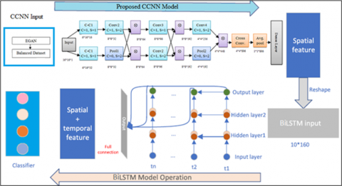
This paper built a deep hierarchical network that integrates the proposed Cross-correlated Convolution Neural Network (CCNN) and Bi-directional LSTM (BiLSTM), named as CCNN-BiLSTM for learning the spatial and temporal aspects of NTD to deal with the difficulty of data features. Because of its strong performance in automatic feature extraction, CCNN has steadily been applied to network identification. Considering that sample attacks are time sequence data, which is intra-dependent. Automatically measure the time sequence features, this research work used BiLSTM for learning. The main contribution of this research work is given below.
(1) To overcome the data imbalance problem, the research developed an Adversarial Sampling strategy. Enhanced Generative Adversarial Networks EGAN is proposed in this research as a way to increase minority sample sizes. In this method created a balanced dataset for model training. Hence, the time for training the model is cut in half.
(2) The deep hierarchical network model, which combines Cross-correlated Convolution Neural Network (CCNN) and BiLSTM, is proposed. This approach extracts the data's features with reliability. The CCNN obtained a model performs better after training.
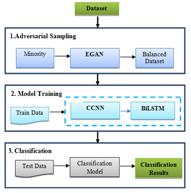
Figure 1. System architecture for proposed NID model
Figure 1 depicts the system architecture of the proposed Network Intrusion Detection (NID) model. To address the imbalance data and the difficulty of the features, the original data is initially applied to Adversarial Sampling process to provide balanced data. Finally, classification is performed in a Deep Hierarchical Network (DHN). It is divided into four sections, which are Adversarial Sampling, model training, and classification.
The performance of the classification model is influenced by the imbalanced data. As a result, this research work employs the EGAN algorithm to raise the minority samples.
The problem of low detection rate and difficulty of feature learning in a small number of attack categories (U2R; R2L) are not considered in existing intrusion detection. Hence to handle the issue of feature learning in a small number of attack categories, a generative adversarial network method is proposed to identify more features.
The NID dataset instances contain too many 0 elements that are not helpful for network learning and can speed up the convergence of the network. This is not resolved by the data normalization approaches. Hence to prevent the over fitting problem due to 0 elements, a cross-correlation-feature layer is included in the DNN model. The proposed CCNN and BiLSTM are help to retrieve the data’s temporal and spatial properties to increase the classification accuracy.
Resistance training, created a model with better classification performance, and the model is utilized to test set categorization, yielding better classification outcomes.
3.1 Balanced data set construction using adversarial sampling
A typical imbalanced data classification challenge is NTD, which consists of a minimum number of anomalous traffic and significant volume of regular traffic. Although the prediction is accurate in this situation, the overall error is minimized. This work proposed an Enhanced Generative Adversarial Networks (EGAN), which is enhanced by incorporating an inference network into the conventional GAN model. It allows the classification methods to consider the impact inputs from both data and latent space. It learns the latent representation by combining autoencoder structure with a normal GAN framework. The generative net (G) and the discriminative net (D) are the two kinds of network in GAN. In the training stage generative net (G), the G attempts to generate fake data based on input priority during the training stage. The traditional GAN has some significant issues, which are:
Model parameters fluctuate and destabilize and never coverage;
The generator fails, resulting in a restricted number of sample variations;
The discriminator becomes too successful, and the generating gradient vanishes, leaving the learner with no information;
Over fitting is caused by an imbalance between the discriminator and the generator.
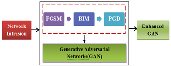
Hyper - parameter choices are quite delicate. To overcome these issues, this research work combined Basic Iteration Method (BIM), Fast Gradient Sign Method (FGSM), and Projected Gradient Descent (PGD) algorithms. Initially, the FGSM method is to create an adversarial sample from NSL-KDD Dataset. This technique performed an updating of 1-step gradient in the direction of the gradient for each dataset input. The BIM is the second method [26], which performs a greater optimization of the FGSM over multiple rounds with modest alterations [27]. Any feature of the input parameters is cropped in any cycle to avoid too significant a change on each feature. The PGD is a version of the FGSM attack that does not include the FGSM's random start characteristic [28]. For identifying such adversarial examples, PGD is an effective first-order technique, which also used to address optimization issues involving the simultaneous minimization of several objective functions. To generate the adversarial samples PGD can produce more accurate perturbation by using a uniform random perturbation as an initialization. Then it runs in the multiple BIM iterations to identify the adversarial samples. All these three approaches rely on the model gradient and are model dependent. Procedure was repeated with the BIM and PGD adversarial samples for getting higher accuracy.
Figure 2. Adversarial sampling by EGAN using EGSM, BIM and PGD process
The proposed EGAN is used in the Adversarial Sampling process, which aims to raise the minority samples in the imbalanced NTD. Figure 2 represents the Adversarial Sampling Process. EGAN is used of three neural networks: a generator (g), an encoder (i), and a discriminator (d), with g and i forming the autoencoder. The encoder i compresses real data samples (a) into a latent representation (b), while the decoder g reconstructs the encoded data back into the original data (a). By learning the joint posterior distribution p(a|b), this autoencoder structure can reconstitute the original data, improving the model's stability by decreasing mode collapse caused by GAN's inability to infer the mapping of actual data to latent data. The auto encoder may also assist with operations at the level of abstraction by utilizing the encoder to learn the inference (a b), where a (a) represents actual data spaces and (b) represents latent spaces, of the latent representation of high-dimensional data spaces. In terms of the advantages of learning latent representations in Eq. (1):
$\max _{g, i} \min _g e(d, i, g)=i_{a \sim p a}\left[i_{a \sim p i}(. \mid a)[\log d(a, b)]\right]+i_{b \sim p b}\left[i_{a \sim p g}(. \mid b)[1-\log d(a, b)]\right]$
$=i_{a \sim p a}[\log d(a, i(a))]+i_{b \sim p b}[1-\log d(g(b), b)]$ (1)
where, $p a$ and $p b$ are the sharing over the data. The $p i(. \mid a), p a(. \mid b)$ and $p g(. \mid a)$ and $p b(. \mid b)$ are the joint distributions of $p i, p a, p g$, and $p b$, which are demonstrated using encoder and generator.
Algorithm 1 Adversarial Sampling Algorithm
|
Input: NSL-KDD dataset Output: Detection result Procedure: Step 1. Start the process Step 2. Generate the adversarial samples using FGSM Step 3. Update the direction of the gradient sign for each input dataset Step 4. Assign BIM for multiple rounds with modest alterations for FGSM Step 5. Generate the adversarial samples using PGD Step 6. To run multiple BIM iterations to identify the adversarial samples Step 7. From the training set, collect all minority class samples. Step 8. Initialize the discriminator d, encoder i, the generator g Step 9. Sort the sample into training subsets randomly using e(d, i, g) Step 10. For i=1training do Step 11. Assign the majority samples into subset Step 12. For g do Step 13. g Generate the imitation dataset Step 14. Send generated data to d; Step 15. End Step 16. Ford do Step 17. d classifies data including the imitation dataset and original dataset Step 18. End Step 19. End Step 20. Enhance the finally synthesized minority sample to obtain the first balanced dataset. Step 21. End |
3.2 CCNN for extraction of spatial features
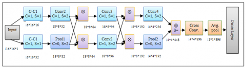
The proposed Cross-correlated Convolution Neural Network (CCNN)can automatically extract the features of objects better than traditional methods. The features delivered from EGAN is given to the CCNN for training. Because the characteristics have spatial locality at dissimilar places, pooling layers must be used to assemble the information of the characteristics at different positions to some extent to eliminate the dimension and overfitting should be avoided. As a result, CCNN is well suited to extracting geographical information from large networks' NTD.
Figure 3. CCNN network structure model
Figure 3 depicts the CCNN network structure model. The procedure for mining the spatial characteristics using CCNN is given below The CCNN the introduction of the idea of local perception, the convolution kernel can be shared by all neurons, and the collection of weights is determined by the number of convolution kernels. As a result, the collection of weights is drastically eliminated, while computational efficiency is greatly improved. The convolution function is denoted by the symbol in Eq. (2):
$h_t=C\left(h_{t-1} \otimes h_t+b_a\right)$ (2)
where, ha is the character map of layer, bias layer is $a,(a D 1 ; 2 ;:: n) b_a$, and $\otimes$ is the convolution function and c (x) is the activation function. This research work used ReLU as CCNN activation function. After the convolution, the pooling layer combines the features in the local neighborhood to generate new features. It is able to decrease the feature map ht size and preventing over-fitting, which is defined in Eq. (3) as follows:
$h_t=\operatorname{pool}\left(h_{t-1}\right)$ (3)
where, ht must be transformed into a vector after numerous convolution and pooling layers. The completely linked layer can then be used to produce output ua. As a result, we can extract the geographical properties of the NTD using CCNN. While CCNN can extract spatial characteristics effectively, it struggles to learn sequence correlation information and cannot overcome the problem of long-term information dependence. As a result, network intrusion detection accuracy using solely CCNN has to be increased.
3.3 Extraction of temporal features by BiLSTM
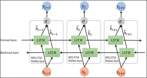
The LSTM contains a memory module which can decide whether to store information in memory and when to forget it LSTM can effectively extract time series with significantly larger intervals and delays, effectively resolving gradient disappearance and training challenges. However, the importance of information after characteristics is not completely taken into consideration because the LSTM could only accept the sequence data in one way. As a result, BiLSTM is utilized instead of LSTM to present the upcoming information. Figure 4 demonstrates Fundamental Structure of BiLSTM.
Figure 4. Fundamental structure of BiLSTM made up using stacking of 2 LSTM
Figure 4 demonstrates Fundamental Structure of BiLSTM. The hidden loop layer, input layer, and an output layer comprise a standard LSTM network framework. The cyclic hidden layer, unlike the standard recurrent neural network, is mostly made up of nodes that represent neurons [23]. The memory module is the fundamental element of the cyclic hidden layer LSTM. The input gate, forget gate, and output gate are among the 3 adaptive multiplication gating units of this memory module. Each neuron node in the LSTM performs the following mathematical operation:
The input gate is activated at time t according to the previous cell's output result ha in represent in Eq. (4). The current input xt decides whether or not to use calculation to update the current information in the cell. The weight is B, while the bias of neurons is b:
$h_t=\operatorname{sigmoid}\left(B_i \cdot\left[h_{t-1}, x_t\right]+b_i\right)$ (4)
The information is retained or discarded using a forget gate, and the last instantaneous hidden layer output ti-1 and the input present time in Eq. (5):
$C_i=\operatorname{sigmoid}\left(B_c \cdot\left[h_{t-1}, x_t\right]+b_c\right)$ (5)
The present value of a potential memory cell is determined by the previous moment's output result ti-1 and input data of the LSTM hidden layer cell. The present value of a potential cell Si and its state Si-1, as well as the forget gate and input gate are currently altering the memory cell state value Si. The unique feature is the element-by-element matrix multiplication present in Eq. (6) and Eq. (7):
$y_i=\tanh \left(B_S \cdot\left[h_{t-1}, x_t\right]+b_S\right)$ (6)
$y_i=C_i+S_{i-1}+h_t * S$ (7)
Calculate the output gate ot, which is utilized to regulate thevalue of the cell status. The last cell's output is ht that can be written as Eq. (8) and Eq. (9):
$o_t=\operatorname{sigmoid}\left(W_0 \cdot\left[h_{t-1}, x_t\right]+b_O\right.)$ (8)
$h_t=o_t \tanh \left(S_t\right)$ (9)
The BiLSTM is made up of 2 LSTM networks, one backwardand the otherforward. The forward LSTM hidden layer is in charge of extracting forward features, while the backward one is in charge of extracting backfeatures in Eq. (10), Eq. (11) and Eq. (12):
$h_t^{\text {backward }}=L S T M^{\text {backward }}\left[h_{t-1}, x_t\right]+S_{t-1}$ (10)
$h_t^{\text {forward }}=L S T M^{\text {forward }}\left[h_{t-1}, x_t\right]+S_{t-1}$ (11)
$H_t=\left[h_t^{\text {backward }}, h_t^{\text {forward }}\right]$ (12)
Prior and after it is applied, the BiLSTM model can effectively understand the importance of every attribute in the sequence information. As a result, more detailed feature information is gathered. BiLSTM's state at time t comprises both forward and backward output [22].
3.4 Enhanced deep correlated hierarchical model
An innovative CCNN was proposed in this research work to improve assessment metrics of imbalanced abnormal traffic data classification in intrusion detection. Finally, we offer some modified variants of the CCCN that may balance detection efficiency and time efficiency to address the algorithm's time efficiency. In the experimental part, we concentrate on enhancing each category of imbalanced anomalous flow data evaluation metrics rather than the total evaluation metrics. By merging CCNN and BiLSTM networks in hierarchical network architecture, the temporal and spatial elements of traffic data may be obtained concurrently. Due to the differences in the CCNN and BiLSTM inputs, the derived spatial characteristics are altered at the CCNN output to fit the BiLSTM network's input. In the CCNN based BiLSTM method has some issues, which are CCNN lacks the capacity to be spatially independent to the input data and does not encode the object's location and orientation.
Both CCNN and BiLSTM are deep learning techniques that are representational. The Figure 5 gives DHN. In the spatial dimension, CCNN may retrieve data characteristics. BiLSTM has the property of retaining relevant historical data for an extended period and achieving data feature extraction at the temporal level. It is vital to examine the feature connection at the spatial level while extracting features for a network intrusion detection system, in addition to measuring the law of change at the temporal level. As a result, this article used CCNN and BiLSTM to retrieve the features before building a DHN. All convolution kernels in the CCNN are 3*3 in size because a lesser convolution kernel can efficiently lower the model's difficulty Furthermore, the larger convolution kernel's comparable responsive field can be obtained by stacking multilayer 3*3 convolution kernels.
Figure 5. Enhanced deep correlated hierarchical structure model
Assuming that Xa-1 is the current layer's input feature map and that the convolution kernel's input size is 3*3, the current layer's output feature map Xa-1 is stated as Eq. (13):
$Y_a=\omega_a * X_{a-1}+b_a$ (13)
The letter ba stands for the bias word. Due to the huge discrepancy in the distribution of flow data samples from different categories, the network adapts effectively to anomalous categories with large sample sizes for highly imbalanced abnormal own data, but the detection impact is often poor for own with few samples. Batch normalization (BN) was used to prevent overfitting [20]. BN reduces the internal covariate shift of the input data, which speeds up the convergence of the training deep network model. BN decreases the correlation of each feature dimension when dealing with unbalanced data, allowing the network to quickly comprehend the categories despite tiny sample sizes. By computing the mean and variance of the samples in an input mini-batch, the data for that mini-batch is normalized. The following is the BN transformation procedure in Eq. (14) and Eq. (15):
$\mu_D=\frac{1}{N} \sum_{a=1}^n y_a$ (14)
$\sigma_D^2=\frac{1}{n} \sum_{a=1}^n\left(y_a+\mu_D\right)^2$ (15)
The mean $\mu_D$ and variance $\sigma_D^2$ of the mini-batch are calculated for each of the $n$ input examples, and the variance and mean are then normalized. The unique procedure is as follows in Eq. (16):
$\widehat{y_a}=\frac{y_a-\mu_D}{\sqrt{\sigma_D^2+\varepsilon}}$ (16)
where, $\mu_D$ represents the mean of all examples in a less-feature batch's dimensions, and $\sigma_D^2$ represents the variance of whole examples in the less-batch. To obtain $\widehat{y_a}$, the example $y_a$ is normalised by $\mu_D$ and $\sigma_D^2$. The normalize procedure is used in every input layer to ensure that all input data has the same distribution regardless of sample variability. The features are scaled and moved to increase the generalization of new data by introducing two learnable parameters and requiring the model to learn the original sample distribution to improve the resilience of network learning present in Eq. (17):
$D N_{\gamma, \beta}\left(y_a\right)=\gamma^{y_a}+\beta$ (17)
The nonlinearity is added using an activation function after the data has been batch normalized. All activation functions in our network structure use the ReLU function to speed up network convergence and resolve the impacts of gradient is-appearance and gradient explosion. As a result, the last output feature map is written as Eq. (18):
$z_a=g\left(D N_{\gamma, \beta}\left(\omega_a * Y_{a-1}+b_a\right)\right)$ (18)
The activation function is denoted by the letter g. Finally, we utilize the Softmax function for our classification, and each category's sample output is stated as Eq. (19):
$x_a=\frac{c^{z_a}}{\sum_{d=1}^e c^{2^d}}$ (19)
Algorithm 2 Deep Correlated Hierarchical Model
|
Input: NSL-KDD dataset. Output: Detection Result Procedure: Step 1. Start the process. Step 2. Apply CCNN and BiLSTM for feature extraction and classification. Step 3. Send balanced NSL-KDD data into enhanced DHN Step 4. For CCNN do Step 5. Apply Cross-correlation layer Step 6. Apply convolutional layer $h_t=C\left(h_{t-1} \otimes h_t+b_a\right)$ Step 7. Extract spatial feature Step 8. End Step 9. For BiLSTM do Step 10. Apply BiLSTM in the enhanced DHN Step 11. Set forward and backward LSTM $\mathrm{LSTMH}_t=\left[h_t^{\text {backward }}, h_t^{\text {forward }}\right]$ Step 12. Extract temporal feature. Step 13. Apply fully connected layer Step 14. Compute the SoftMax function for output layer Step 15. SofMax layer can learn and classifying the dataset Step 16. End Step 17. End |
Tensor Flow was utilized as the backend in the experiments, which was encoded with Keras and Python under Windows. In this research work, the network model's learning rate was set as 0.001.
4.1 Dataset
The traditional and well-known NSL-KDD benchmark dataset [29] can be used in this research work. This dataset contains the 41- dimensional features that are separated to a thirty-eight-dimensional digital feature, a traffic type label, and a 3-dimensional symbol feature. The label consists of Normal, and four varieties of Remote-to-Local (R2L), Denial of Service (Do’s), Probe and User-to-Root (U2R) attack data. Description of the NSL-KDD dataset is given in Table 1.
Table 1. DescriptionNSL-KDD dataset
|
Type |
Testing |
Training |
|
Normal |
9711 |
67343 |
|
Denial of Service (DoS) |
7458 |
11656 |
|
Remote-to-Local (R2L) |
2754 |
995 |
|
Probe |
45927 |
2421 |
|
User-to-Root (U2R) |
200 |
52 |
4.2 Data preprocessing
The one-shot encoding approach has been used to translate the data containing symbol features in the data set to the digital feature vector because the model's input is a digital matrix. This processing is primarily concerned with the protocol type, service, and aspects of data collection. They are coded separately and have 3, 11, and 70 symbol characteristics, respectively. The three protocol type attributes such as UDP, ICMP, and TCP in the NSL-KDD dataset, are stored as binary vectors (0,0,1), (0,1,0), (1,0,0), and respectively. A normalized processing method is used to consistently and linearly map the value range of each feature within the [0,1] interval, making arithmetic processing and dimension elimination easier.
4.3 Performance measures
This research work used following performance measures that are precision, recall, f-score measure, and accuracy have been used to estimate the performance of the proposed framework. These metrics are represented from Eq. (20) to Eq. (23):
Accuracy $=\frac{T P+T N}{T P+T N+F N+T N}$ (20)
Precision $=\frac{T P}{T P+F P}$ (21)
$\operatorname{Recall}=\frac{T P}{T P+F N}$ (22)
$F-$ Score measure $=2 \cdot \frac{\text { Precision XRecall }}{\text { Precision }+\text { Recall }}$ (23)
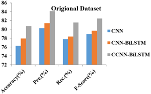
Table 2 shows the Performance Analysis for Original NSL-KDD and Balanced NSL-KDD Dataset. From the observation, the proposed CCNN-BiLSTM classification algorithm gives higher performance ratio than existing algorithms.
Table 2. Performance analysis for classifiers for original NSL-KDD and balanced NSL-KDD dataset
|
Data |
Classifier |
Accuracy(%) |
Pre(%). |
Rec.(%) |
F-Sc.(%) |
|
Original NSL-KDD Dataset |
CNN [22] |
76.28 |
80.25 |
77.76 |
78.89 |
|
CNN-BiLSTM [25] |
77.91 |
81.39 |
78.38 |
79.71 |
|
|
CCNN-BiLSTM |
80.73 |
84.15 |
81.56 |
82.44 |
|
|
Balanced NSL-KDD Dataset |
CNN [22] |
77.68 |
81.65 |
79.16 |
80.29 |
|
CNN-BiLSTM [25] |
79.01 |
82.49 |
79.48 |
80.81 |
|
|
CCNN-BiLSTM |
81.16 |
85.02 |
82.43 |
83.31 |
Figure 6. Performance analysis of classifiers for original NSL-KDD dataset
Figure 6 gives the Performance Analysis of Classifiers for Original NSL-KDD Dataset. From the experimental results, it is observed that the proposed CCNN-BiLSTM classification algorithm produces 81.16,85.02,82.43,83.31 for {Accuracy, Precision, Recall, F-Score} with respect to original NSL-KDD Dataset.
Figure 7. Performance analysis of classifiers for balanced NSL-KDD dataset
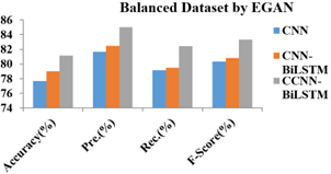
Figure 7 presents the Performance Analysis of Classifiers for Balanced NSL-KDD Dataset. From the experimental results, it is noticed that the proposed CCNN-BiLSTM classification algorithm 80.73, 84.15, 81.56, 82.44 for {Accuracy, Precision, Recall, F-Score} with respect to balanced NSL-KDD Dataset.
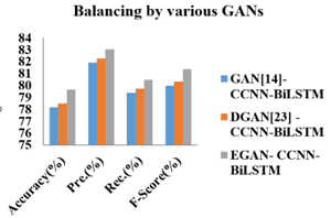
Table 3 represents the Performance Analysis for CCNN-BiLSTM for balanced by existing and proposed balancing methods. The integrated Adversarial Sampling (existing GAN [14], DGAN [23], and proposed EGAN) algorithms and adversarial sampling (proposed CCNN-BiLSTM) algorithm results are given in above table. From the observation, the proposed EGAN algorithm achieves algorithm gives higher performance ratio than existing algorithms.
Figure 8. Performance analysis for original NSL-KDD dataset
Figure 8 illustrates the Performance Analysis for various GANs. From the experimental results, it is observed that the proposed CCNN-BiLSTM algorithm yields 79.63, 83.05, 80.46, 81.34 for {Accuracy, Precision, Recall, F-Score} with respect to balanced NSL-KDD Dataset balanced by EGAN.
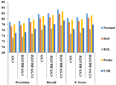
Table 4 represents the Performance Analysis of Classifiers for each class in the NSL-KDD Dataset. From the experimental results, it is noticed that the proposed EGAN-CCNN-BiLSTM classification algorithm gives higher performance ratio than existing algorithms.
Figure 9. Performance Analysis of Classifiers for each class in the NSL-KDD dataset
Table 3. Performance analyses for CCNN-BiLSTM for various GANS
|
Data |
Adversarial Sampling |
Accuracy |
Pre. |
Rec. |
F-Sc. |
|
Original NSL-KDD Dataset |
GAN[14]-CCNN-BiLSTM |
78.14 |
81.93 |
79.38 |
79.98 |
|
DGAN[23]-CCNN-BiLSTM |
78.48 |
82.27 |
79.72 |
80.32 |
|
|
|
EGAN-CCNN-BiLSTM |
81.18 |
84.62 |
82.01 |
82.89 |
Table 4. Performance analysis of classifiers for each class in the NSL-KDD dataset
|
Performance Factors |
Classifiers |
Normal |
DoS |
R2L |
Probe |
U2R |
|
Precision(%) |
CNN [22] |
78.84 |
77.34 |
73.29 |
78.14 |
74.94 |
|
CNN-BiLSTM [25] |
79.18 |
77.68 |
73.63 |
78.48 |
75.28 |
|
|
CCNN-BiLSTM |
80.33 |
78.83 |
74.78 |
79.63 |
76.43 |
|
|
Recall (%) |
CNN [22] |
81.68 |
80.18 |
76.13 |
80.98 |
77.78 |
|
CNN-BiLSTM [25] |
82.02 |
80.52 |
76.47 |
81.32 |
78.12 |
|
|
CCNN-BiLSTM |
83.28 |
81.78 |
77.73 |
82.58 |
79.38 |
|
|
F-Score (%) |
CNN [22] |
80.28 |
78.78 |
74.73 |
79.58 |
76.38 |
|
CNN-BiLSTM [25] |
80.62 |
79.12 |
75.07 |
79.92 |
76.72 |
|
|
CCNN-BiLSTM |
81.88 |
80.38 |
76.33 |
81.18 |
77.98 |
Figure 9 presents the Performance Analysis of Classifiers for each class in the NSL-KDD Dataset. From the experimental results, it is noticed that the proposed EGAN-CCNN-BiLSTM classification algorithm achieves Precision rate 80.33, 78.83, 74.78, 79.63, 76.43, Recall rate 83.28, 81.78, 77.73, 82.58, 79.38 and F-Score rate 81.88, 80.38,76.33, 81.18, 77.98 for each class {Normal, Do’s, R2L, Probe and U2R} in NSL-KDD Dataset.
Generally, all methods suffer from low classification accuracy when applied to U2R and R2L. For starters, training sets for attack types typically have very few examples. The classifiers place less emphasis on these types of assaults during training. Even though there is no silver bullet for this problem, the presented proposed approach significantly raises the detection rate on U2R.This demonstrates that the approach proposed in this paper successfully addresses the issues of a low minority detection rate caused by an uneven distribution of data. In light of this, our proposed approach addresses the difficulties of data imbalance in IDS deployment. The proposed work can be used in any real time network to find even less frequently occurred attacks.
A robust intrusion detection system is proposed, which is performed based on the mixture of Adversarial Sampling and a DHN is presented and explained in this research. To begin, EGAN to build a balanced dataset. It can minimize the model's training time in half and, to some extent, overcome the problem of insufficient training from imbalanced data. In addition, for complicated, multivariate cyber threats, a network data preparation approach is devised, which is appropriate for the proposed model. Finally, categories the input data, CCNN and BiLSTM are used to construct a hierarchical network model. Using the exceptional properties of deep learning, the model collects features automatically through periodic multi-level learning. The NSL-KDD dataset is used in this research work for analyzing the performance of the proposed system. From the performance results, it is observed that the proposed EGAN-CCNN-BiLSTM algorithm gives a higher performance ratio than existing algorithms. However, a new class of attacks that generated by adversarial inputs not only misleading target DNNs but also deceiving their coupled interpretation models. An empirical evidence mechanism can be used to reduce the prediction-interpretation gap.
[1] Bijone, M. (2016). A survey on secure network: Intrusion detection and prevention approaches. American Journal of Information System, 4(3): 69-88. https://doi.org/10.12691/ajis-4-3-2
[2] Weller-Fahy, D.J., Borghetti, B.J., Sodemann, A.A. (2015). A survey of distance and similarity measures used within network intrusion anomaly detection. IEEE Communications Surveys & Tutorials, 17(1): 70-91. https://doi.org/10.1109/COMST.2014.2336610
[3] Keung, G.Y., Li, B., Zhang, Q. (2012). The intrusion detection in mobile sensor network. IEEE/ACM Transaction on Networking, 20(4): 1152-1161. https://doi.org/10.1109/TNET.2012.2186151
[4] Huang, C., Min, G., Wu, Y., Ying, Y., Pei, K., Xiang, Z. (2022). Time series anomaly detection for trustworthy services in cloud computing systems. IEEE Transactions on Big Data, 8(1): 1-13. https://doi.org/10.1109/TBDATA.2017.2711039
[5] Maghraby, R.T., Elazim, N.M.A., Bahaa-Eldin, A.M. (2017). A survey on deep packet inspection. 12th International Conference on Computer Engineering and Systems (ICCES), pp. 188-197. https://doi.org/10.1109/ICCES.2017.8275301
[6] Vlăduţu, A., Comneci, D., Dobre, C. (2017). Internet traffic classification based on flows statistical properties with machine learning. International Journal of Network Management, 27(3): e1929. https://doi.org/10.1002/nem.1929
[7] Zheng, K., Cai, Z., Zhang, X., Wang, Z., Yang, B. (2015). Algorithms to speedup pattern matching for network intrusion detection systems. Computer Communication, 62: 47-58. https://doi.org/10.1016/j.comcom.2015.02.004
[8] Zhang, J., Chen, X., Xiang, Y., Zhou, W., Wu, J. (2015). Robust network traffic classification. IEEE-ACM Transaction on Networking, 23(4): 1257–1270. https://doi.org/10.1109/TNET.2014.2320577
[9] Aljawarneh, S., Aldwairi, M., Yassein, M.B. (2018). Anomaly-based intrusion detection system through feature selection analysis and building hybrid efficient model. Journal of Computational Science, 25: 152-160. https://doi.org/10.1016/j.jocs.2017.03.006
[10] Thaseen, I.S., Kumar, C.A. (2017). Intrusion detection model using fusion of chi-square feature selection and multi class SVM. Journal of King Saud University-Computer and Information Sciences, 29(4): 462-472. https://doi.org/10.1016/j.jksuci.2015.12.004
[11] Kevric, J., Jukic, S., Subasi, A. (2017). An effective combining classifier approach using tree algorithms for network intrusion detection. Neural Computing and Applications, 28: 1051-1058. https://doi.org/10.1007/s00521-016-2418-1
[12] Ahmad, I., Basheri, M., Iqbal, M.J., Rahim, A. (2018). Performance comparison of support vector machine, random forest, and extreme learning machine for intrusion detection. IEEE Access, 6: 33789-33795. https://doi.org/10.1109/ACCESS.2018.2841987
[13] Zhang, L., Zhang, Q., Zhang, L., Tao, D., Huang, X., Du, B. (2015). Ensemble manifold regularized sparse low-rank approximation for multi view feature embedding. Pattern Recognition, 48(10): 3102-3112. https://doi.org/10.1016/j.patcog.2014.12.016
[14] Maithem, M., Al-sultany, G.A. (2017). Network intrusion detection system using deep neural networks. Journal of Physics: Conference Series, 1804(1): 012138. https://doi.org/10.1088/1742-6596/1804/1/012138
[15] Yin, C., Zhu, Y., Fei, J., He, X. (2017). A deep learning approach for intrusion detection using recurrent neural networks. IEEE Access, 5: 21954-21961. https://doi.org/10.1109/ACCESS.2017.2762418
[16] Shone, N., Ngoc, T.N., Phai, V.D., Shi, Q. (2018). A deep learning approach to network intrusion detection. IEEE Transactions on Emerging Topics in Computational Intelligence, 2(1): 41-50. https://doi.org/10.1109/TETCI.2017.2772792
[17] Nevat, I., Divakaran, D.M., Nagarajan, S.G., Zhang, P., Su, L., Ling Ko, L., Thing, V.L. (2018). Anomaly detection and attribution in networks with temporally correlated traffic. IEEE/ACM Transaction on Networking, 26(1): 131-144. https://doi.org/10.1109/TNET.2017.2765719
[18] Kim, J., Kim, J., Le, H., Thu, T., Kim, H. (2016). Long short term memory recurrent neural network classifier for intrusion detection. International Conference on Platform Technology and Service (PlatCon), pp. 1-5. https://doi.org/10.1109/PlatCon.2016.7456805
[19] Bamakan, S.M.H., Wang, H., Shi, Y. (2017). Ramp loss K-support vector classification-regression; a robust and sparse multi-class approach to the intrusion detection problem. Knowledge-Based System, 126(10): 113-126. https://doi.org/10.1016/j.knosys.2017.03.012
[20] Yan, B., Han, G., Huang, Y., Wang, X. (2018). New traffic classification method for imbalanced network data. Journal of Computer Applications, 38(1): 20. https://doi.org/10.11772/j.issn.1001-9081.2017071812
[21] Zhang, X., Chen, J., Zhou, Y. (2019). A multiple-layer representation learning model for network-based attack detection. IEEE Access, 7: 91992-2008. https://doi.org/10.1109/ACCESS.2019.2927465
[22] Zhang, Y., Chen, X., Jin, L., Wang, X., Guo, D. (2019). Network intrusion detection: Based on deep hierarchical network and original flow data. IEEE Access, 7: 37004-37016. https://doi.org/10.1109/ACCESS.2019.2905041
[23] Zhang, H., Yu, X., Ren, P., Luo, C., Min, G. (2019). Deep adversarial learning in intrusion detection: A data augmentation enhanced framework. CoRR. https://doi.org/10.13140/RG.2.2.19731.73762
[24] Roshan, S., Miche, Y., Akusok, A., Lendasse, A. (2018). Adaptive and online network intrusion detection system using clustering and extreme learning machines. Journal of the Franklin Institute, 355(4): 1752-1779. https://doi.org/10.1016/j.jfranklin.2017.06.006
[25] Jiang, K., Wang, W., Wang, A., Wu, H. (2020). Network intrusion detection combined hybrid sampling with deep hierarchical network. IEEE Access, 8: 32464-32476. https://doi.org/10.1109/ACCESS.2020.2973730
[26] Goodfellow, I.J., Shlens, J., Szegedy, C. (2015). Explaining and harnessing adversarial examples. International Conference on Learning Representations (ICLR). https://doi.org/10.48550/arXiv.1412.6572
[27] Kurakin, A., Goodfellow, I., Bengio, S. (2016). Adversarial machine learning at scale. arXiv preprint arXiv:1611.01236. https://doi.org/10.48550/arXiv.1611.01236
[28] Madry, A., Makelov, A., Schmidt, L., Tsipras, D., Vladu, A. (2017). Towards deep learning models resistant to adversarial attacks. arXiv preprint arXiv:1706.06083. https://doi.org/10.48550/arXiv.1706.06083
[29] Tavallaee, M., Bagheri, E., Lu, W., Ghorbani, A. (2009). A Detailed Analysis of the KDD CUP 99 Data Set, Submitted to Second IEEE Symposium on Computational Intelligence for Security and Defense Applications (CISDA). https://www.unb.ca/cic/datasets/nsl.html.