Mohammed Rashad Baker* | Zuhair Norii Mahmood | Ehab Hashim Shaker
© 2022 IIETA. This article is published by IIETA and is licensed under the CC BY 4.0 license (http://creativecommons.org/licenses/by/4.0/).
OPEN ACCESS
In recent years, the highly boosting development in e-commerce technologies made it possible for people to select the most desirable items from shops and stores worldwide while being at home. Credit card frauds transactions are common nowadays because of online payments. Online transactions are the root cause of fraudulent credit card activity, bringing enormous financial losses. Financial institutions must install an automatic deterrent mechanism to check these fraudulent actions. The fraudulent transactions do not follow a specific pattern and continuously change their shape and behavior. This paper aims to use ensemble learning with supervised Machine Learning (ML) models to predict the occurrence of fraud transactions. The experimental study has been evaluated on the open-source Kaggle credit card fraud detection dataset. The performance of the proposed model is measured in terms of accuracy score, confusion matrix, and classification report. The results were state-of-the-art using the voting ensemble learning technique shows that it can be get the best results using PCA with 100.0% accuracy, 97.3% precision, 73.5% recall, and 83.7% f1-score against other ML classifiers.
fraud detection, dimensionality reduction, machine learning, ensemble learning, upsampling
In the modern era, the revolution of advanced technology makes life easy in business and products dealings in the form of e-commerce. However, e-commerce is also facing a grave credit card fraud detection issue. Credit card fraudulent activities are increasing day by day. Nowadays, small and large enterprises use credit cards as a style of payment [1]. Credit card fraudulent activity is found in almost all organizations like the automobile industry, appliances industry, banks, etc. Machine Learning (ML) and data mining have been applied to fraud detection in credit card transactions; however, these approaches could not achieve promising results. There is a need for an effective and efficient way to detect fraudulent activity instantly to prevent this alarming financial loss situation [2].
Credit card fraud detection is an offensive activity taken by an unauthorized person to steal credentials and use the card for his purposes. The credentials can be taken by using software applications as the user makes the credit card transaction online. Credit card fraud detection can also occur when fraudsters physically give a credit card to the merchant. The use of ML techniques brought a revolution in every walk of life, and research is showing their efficiency because of promising results. ML combines statistical and computer-based algorithms that allow the computer to perform without manually coding in a programming language. ML models take input as labeled data to learn complex patterns and inferences on unlabeled data [3].
ML can provide a trustworthy and efficient method for addressing complicated challenges in real-world applications. For instance medicine [4, 5], Information security [6], gaming [7, 8], sports [9], and energy consumption [10] and many others.
ML also plays a key role in financial data analysis [11]. Researchers have addressed the issue of credit card fraud detection through ML algorithms. Credit Card fraud detection is common due to the high number of online transactions [12]. As technology is making progress, the loophole is also increasing. Fraudsters are designing new approaches to detect the secret information related to a credit cards. Credit card fraud detection is a hot domain for researchers as the datasets are hard to get due to customers' financial privacy. The publicly available datasets are imbalanced due to the high number of routine transactions. The transaction patterns also change their statistical properties concerning time. It is hard to recognize fraudulent transactions in the recent era because of their dynamic nature, i.e., most of them are made to look like legitimate transactions [12, 13].
In this paper, we deal with the problem of credit card detection using a publicly available imbalanced dataset on Kaggle. We address the problem using Synthetic Minority Oversampling Technique (SMOTE) oversampling and the majority voting ensemble learning technique on various ML classifiers. These classifiers include Bagging, Decision Tree (DT), Random Forest (RF), AdaBoost, Logistic Regression (LR), Naive Bayes (NB), and Support Vector Machine (SVM).
1.1 Problem statements
Various ML techniques have been investigated to assist stakeholders' decisions in the case of financial transactions and investments. The fraudulent financial activity is challenging for community regulators and the government to address. The government institution generates fraudulent financial data only to verify the critical financial loss of a large number of investors. Additionally, the authors remark that most firms do not share their financial data for research purposes due to customer security and privacy concerns.
The banks and governmental financial institutions have been taking steps to subdue fraudulent activity for the last decade by using different ML techniques. However, each technique suffers a setback because it has to be more than 99% accurate. A single false positive can result in substantial financial loss to the client.
1.2 Research questions
Here we have two research questions:
RQ. 1: Is the majority voting ensemble learning technique better than the other credit card fraud detection approaches?
RQ. 2: Which of applied oversampling techniques can be utilized for credit card fraud detection to give more reliable result?
The contributions of the proposed approach in this paper are:
• This study evaluated a demanding experimental approach and compared our results with the different state-of-the-art ML models. The proposed approach identifies the weakness in tackling the credit card fraud detection of real-world problems. Below is the list of our contributions work.
• To our knowledge, the proposed approach is the first ensemble learning approach used in fraudulent activity detection in credit card transactions.
• The proposed approach has been compared with the supervised ML algorithms and found that the proposed approach beats the supervised ML models.
• In this study, an experimental approach with a balanced and imbalanced dataset is conducted, and evaluated the results that provide information about the biasness of the class instances.
The remaining portion of the paper is organized as follows; Section 2 is about the literature review, Section 3 is about methodology, Section 4 results, and discussion. Section 5 contains concludes and future direction.
Fraud detection is a famous and it was practiced in different domains. Abdallah et al. [14], presented detailed descriptions of the wide range of fraud topics, comprising credit card fraud and telecommunication [15, 16], automobile insurance fraud [17, 18], and online auction fraud [19]. According to the survey document, banks employ most fraud detection techniques. Size and unequal distribution are potential issues with fraudulent transactions in the financial sector. The researchers spent considerable time resolving the data's unequal distribution. However, their proposed approaches starts fraud detection models by randomly selecting an actual number of transactions from the non-fraudulent transactions [20-22]. Personal data protection and privacy rules made the research problem complex to work on real banking data. Lucas et al. [23], used anonymous data to solve the issue of real-life data. This study focuses on credit card numbers, terminal-id, and reference numbers. They were based on assumptions and were mimicked to create synthetic transactions.
Pumsirirat and Yan [24], emphasized the unsupervised method as a better approach as fraud detection methods constantly change. The training and test split ratios were 80% and 20%, with 21 features. Autoencoders and Restricted Boltzmann Machine (RBM) were used to detect anomalies in transactions. The Area Under Curve (AUC) was 0.960 on the European dataset. The equal class distribution in the target variable is a critical issue to avoid the miss-classification problem since fraud transactions are uncommon in most datasets. ML algorithms can easily find their regularities in large datasets compared to small datasets [25]. The overlapped attribute values also create problems in a large number of transactions. The minority classes become linearly separable and create more minor problems for the algorithms even if the data is highly unbalanced [26]. Hadoop and MapReduce paradigms are also utilized by executing the negative selection algorithm for credit card fraud detection [27]. Quah and M. Sriganesh [28], used unsupervised self-organizing maps to identify fraudulent activity in credit card transactions in real time. Kundu et al. [29], presented SSAHA and BLAST's hybrid techniques as profile analyzers and deviation analyzers to detect fraudulent credit card activities.
This study used a deep learning method to help with financial decisions and credit card fraud analysis. Deep learning is good at many things, like image processing and other data science fields [30]. Jurgovsky et al. [31], showed the Long Short Term Memory (LSTM) network for credit card fraud detection, they used a sequence classification task to show how the network works. Fiore et al. [32], employed unsupervised Generative Adversarial Networks (GANs) to create fictitious persons and improve credit card fraud detection by tackling the problem of an imbalanced dataset. A hybrid method that used the unsupervised outlier values to enhance the set of features in the fraud detection classifier was used. The main thing this method does is set up and figure out how to define outlier scores at different levels of granularity. The proposed method results show that this made it easier to find credit cards [33]. Carcillo et al. [34] devised a way to solve the imbalance, non-stationary, and feedback latency problems. They used the Scalable Real-Time Fraud Finder (SCARFF) technique, which used big data and ML. The performance evaluation of a large dataset shows that the proposed method is efficient, scalable, accurate, and easy to use. A new way to look for fraud is shown that uses the Discrete Fourier Transform (DFT) [35]. This method may be able to fix an imbalance in class distribution and lessen the amount of data heterogeneity.
Data imbalance is a challenging issue in fraud detection. The difference between a majority and minority sample data distribution is highly imbalanced and a big hurdle in fraudulent activity detection [36, 37]. The traditional ML classifiers show poor output on imbalanced data and cannot represent the minority class [38]. Some techniques have been proposed to handle imbalanced data classification, like Resampling techniques [39, 40]. The resampling methods have the disadvantage that it reduces majority class performance. Makki et al. [41], state that credit card fraud is a significant financial loss. To overcome financial loss is time-consuming and expensive. They investigate that imbalance classification is a fundamental cause of misclassification and results in poor performance of ML models. The proposed models are Linear Regression, DTs, ANNs and SVMs trained on balanced datasets and show benchmark results in sensitivity, AUC, precision, recall, and accuracy. Jiang et al. [12], present a novel idea that comprises multiple stages. In the initial step, cardholder transactions are collected, transactions are aggregated based on behavioral patterns, followed by splitting the dataset for train and test. The model is trained on training data and evaluated on test data. The feedback system has been set to know about the unusual patterns. Sohony et al. [42], used the ensemble technique for fraudulent activity detection in credit cards. They investigated that ensemble models of RF show higher accuracy and that neural network models are also better at detecting fraud instances. The ensemble model combines RF and neural networks in the study.
The proposed methodology for credit card fraud detection is shown in Figure 1. The proposed methodolgy consists of four main branches, each comprising two sub-parts. Two sub-parts of each main branch focus on with/without SMOTE oversampling technique combined with ensembling technique. Each sub-part ends with Majority Voting (Hard) Ensembling Technique. The four recommended methods operate independently of each other. The goal here is to determine which of the various assumed approaches could be applied to the dataset with the highest level of accuracy. The purpose of using ensemble techniques is that we need to make our dataset balanced to avoid bias regarding any side of the binary class.
ML classifiers used in the proposed approach are Bagging Classifier, DT, RF, AdaBoost, LR, NB, and SVM. Each main branch is also unique in terms of dimensionality reduction technique. Dimensionality Reduction (DR) is a pre-processing step that gets rid of redundant features, noisy data, and data that's not important to the learning process. It thus improves the accuracy of the learning features and shortens the training time. Dimensionality techniques are Principal component analysis (PCA), Linear Discriminant Analysis (LDA), and Autoencoder. For the autoencoder branch, we have used Min-Max normalization on features of the dataset. The experimental approach has been conducted on Windows operating system with Intel Core i7 10th generation processing with 32 GB RAM. The python programming language is used to implement projects on anaconda (Jupiter Notebook).
Figure 1. Proposed methodology
3.1 Dataset description
The dataset is taken from the open-source platform Kaggle. The dataset consists of 31 attributes and 284807 records. The dataset is highly imbalanced in which minority class "fraud" data points are only 492 while majority classes "non-fraud" data points are 284315. The class imbalance is a significant risk in determining the characteristics of fraud in a transaction pattern. The majority classes are correctly classified by learning more instances of the majority class and ignoring the minority classes, leading to misclassification. In the proposed study, minority class fraud data points are critical to correctly classify.
3.2 Synthetic minority oversampling technique (SMOTE)
SMOTE is a well-known and efficient technique for handling class imbalance issues in various field [43]. The core concept of SMOTE is the synthesis of additional minority samples based on similarity in feature space between existing minority examples. We applied the SMOTE approach to oversample the minority class. SMOTE, or Synthetic Minority Oversampling Technique, is an additional method for oversampling the minority class. Frequently, adding duplicate minority class data to a model does not add any new information. SMOTE synthesizes new instances from the existing data. Consequently, SMOTE examines minority class examples and uses k nearest neighbor to identify a random nearest neighbor; a synthetic instance is then generated at random in feature space.
3.3 Proposed classification models
In the proposed approach, we have used seven ML classifiers. Bagging Classifier, Decision Tree, Random Forest, AdaBoost, Logistic Regression, Naive Bayer, and Support Vector Machine. The selection of these algorithms is used in the literature on the given problem and many other problems. The following section provides a brief underlying mechanics of these algorithms
3.3.1 Logistic regression (LR)
The LR model is used for classification tasks to find a relationship between the probability of an outcome and features [44]. The logistic term is derived from the logit function that used the probability value of 0.5 for the classification method. The LR model contributes to fraud detection based on given features and parameters [45]. The functioning technique of LR resembles the linear regression model, only the difference in calculating the predicted probability of the mutual exclusive event occurring based on multiple external factors. The LR model is a linear model in which the target variable is categorical contrast, the independent variable in LR should be independent of each other. Therefore, the LR model has little or no multicollinearity [46]. The LR model mathematically can be designed to map input variables with two possible output classes, negative and positive classes.
3.3.2 Support vector machine (SVM)
SVM is a powerful predictor classification model that separates the dataset into two training and testing sets [47]. The main goal of the SVM model is to design a model using training data that predicts the test data's target values based on its attributes. SVM model is memory-efficient because it uses a subset of training points. SVM does not perform with noisy datasets with overlapping classes. SVM's main principle is to draw the optimal hyperplane to enhance classification accuracy. SVM is based on statistical learning theory. It is find a linear model that maximizes the margin of hyperplanes [48]. The hyperplane's maximum margin will maximize class separation.
3.3.3 Decision tree (DT)
The DT is different from that of other ML models as it is a non-parametric classification and regression tool [49]. It is represented using a tree-like structure where each internal node represents a feature, and the connection represents the outcome of the feature. The leaf nodes represent class labels. The tree construction is accomplished by dividing the dataset into subsets based on the result of the feature value test. Recursive segmentation is the process of repeating this procedure on each subset obtained from another. Whenever the subset at a point has the same result as the target attribute or when splits no further improves the predictions, then recursion is concluded. Since it does not require domain knowledge or parameter configuration, it is well suited for exploratory knowledge discovery applications. In addition, DTs can handle data with a high degree of dimensionality. As a result, DT classifiers are often accurate in their classifications [50]. The induction of categorization information through DTs is a typical inductive approach.
3.3.4 Random forest (RF)
The RF is an ensemble technique capable of solving classification and regression tasks. RF is a combination of DT classifiers, and its output is the majority vote among the set of tree classifiers [51]. A subset of the whole training set has been selected at random and used to train it for each tree. Unlike other algorithms, the RF algorithm is not susceptible to overfitting. As a result, the error rate it returns can provide an accurate estimation of generalization error (without requiring it to run through a cross-validation procedure). The RF model can handle the categorical and numeric features and even work with missing values and non-scale [52].
3.3.5 Convolution neural network (CNN)
The CNN model is a deep learning model that has a promising contribution to solving imaging types of tasks [53]. The CNN model is a feedforward network consisting of input, convolutional, pooling, and output layers. The CNN model is capable of feature extraction and learning, which is very useful in images. A convolution filter connects a CNN model's output layer to the model's input layer. The dot multiplication function of the convolution filter is utilized to produce multiscale feature extraction using a sliding window technique [54]. The max-pooling layer was used to minimize the complexity of the feature matrix and the network complexity. The convolutional layer is responsible for extracting features from the initial input.
3.3.6 Adaptive boosting (AdaBoost)
AdaBoost is an iterative ensemble learning method that aims to increase the efficiency of binary classifiers by learning their mistakes and turning them into strong ones [55]. AdaBoost uses sequential learning to generate different models sequentially, and successors learn from mistakes that exploit dependency among models by giving high weightage to mislabeled examples.
3.3.7 Naive bayes (NB)
NB is a distinct technique based on the Bayes Theorem and assumes that predictors are independent of one another [56]. It is commonly used for massive datasets because of its simplicity, and it has been shown to outperform even the most advanced classification methods in several cases.
3.4 Majority voting (Hard)
Majority Voting (MV) is an ensemble learning method that integrates the predictions from numerous underlying algorithms into a single forecast [57]. It outperforms any underlying model employed in the method in terms of overall performance. It is engaged in the categorization and regression of data sets. In the case of regression, it takes the average of the predictions from the models. When it comes to classification, the predictions for each predicted label are added together, and the predicted label with the most votes is declared the winner. Hard voting and soft voting are the two techniques of a majority vote for classification that can be used [58]. Hard voting adds up all of the guesses for each predicted label, and the real label is the one that receives the most votes. You can use soft voting to calculate the expected probabilities for each predicted label and then use that information to predict the real label with the highest likelihood.
Consequently, hard voting is reserved for models with clear predicted labels, and soft voting is reserved for models with probabilities belonging to a certain category of labels. In our proposed approaches, we used uniform weights while using the majority class.
This section discusses the first performance metrics, followed by the results of all experiments conducted and their discussion. Three-dimension reduction techniques were utilized: PCA, LDA, and Autoencoder, while the SMOTE approach has been used for oversampling. We have used k-fold with k=3 to accurately report all the experiments' performance. 80% of the data is used for training, and the rest 20% for testing.
4.1 Proposed classification models
To estimate the performance of the proposed approach, accuracy, precision, recall, and f1-score as performance metrics have been used. These are defined as follows:
4.1.1 Accuracy score
Accuracy is the ratio correction prediction out of the total predictions. This metric is considered very important to get accurate results. The accuracy score can illustrate as shown in equation (1):
Accuracy $=\frac{T P+T N}{T P+F P+F N+T N} \times 100$ (1)
4.1.2 Precision
It is the ratio of correctly True positive predictions out of the total True positive predictions. The precision metric can be expressed as shown in equation (2):
Precision $=\frac{T P}{T P+F P}$ (2)
4.1.3 Recall
The ratio correct predicted positive prediction from all observations in an actual class. A recall is also known as sensitivity. The recall metric can illustrate as shown in equation (3):
Recall $=\frac{T P}{T P+F N}$ (3)
4.1.4 F1-Score
F1 Score is the weighted average of Precision and Recall. F1-Score counts false positives and false negatives both to show the output value. F1-Score can illustrate as shown in equation (4):
$F 1-$ score $=2 \frac{\text { Recall } * \text { Precision }}{\text { Recall }+\text { Preicsion }}$ (4)
A False Positive (FP) is a positive result that has a large number of inaccurate examples. In the above equation, TP stands for True positive, which is the number of cases that have been correctly identified. The number of successfully identified examples is denoted by TN, whereas FN denotes the number of incorrectly categorized examples.
4.2 Mathematic text and equations
The main branches used for experimental are four; each main branch has two sub-parts. Each branch's result will be discussed separately, followed by a combined analysis of all four branches.
• Branch-1 is the simplest of all branches as it only focuses on results with and without oversampling. For oversampling, SMOTE technique for the experiments has been used. Sixteen (16) experiments have been conducted in two sub-parts, with each sub-part consisting of eight (8) experiments. Table 1 presents all the experiments done in Branch-1. The first eight (8) experiments use seven ML classifiers and one Voting ensemble learning technique to perform simple classification. The remaining eight (8) experiments focus on SMOTE, followed by classification using seven (7) ML classifiers and one technique called Voting ensemble learning. If both classes were considered, Random Forest (RF) outperformed in both sub-branches of this branch. However, LR resulted in a lower misclassification rate for fraud (minority) class in the first sub-part, and Adaptive Boost (AdaBoost) resulted in lower classification in the second sub-part. RF performed better than others because the dataset has thirty (30) attributes. These (30) relevant attributes are used to improve learning feature accuracy, reduce the training time, and discard the “Time” column. Bagging, RF and the voting technique are preformed the best accuracy among all classifiers in first sub-part but RF performs better results against other classifiers in second sub-part.
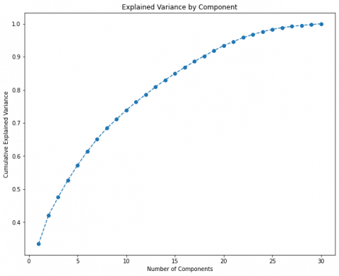
• Branch-2 focuses on Principal Component Analysis (PCA) as a dimensionality reduction technique. For oversampling, SMOTE technique for the experiments has been used. To appropriately enter the number of components into PCA, the elbow approach has been used to plot variance for a number of components.
Figure 2. Components variances applying PCA without using SMOTE
The graph in Figure 2 depicts the variance (y-axis) as a function of the number of components (x-axis). The general norm is to retain 90% of variance. Therefore, in this circumstance, we chose to retain 25 components (features). These features are: "scaled amount", "V1", "V3", "V4", "V6", "V7", "V8", "V9", "V10", "V11", "V12", "V13", "V14", "V15", "V16", "V17", "V18", "V19", "V20", "V21", "V22", "V23", "V24", "V25", and "V27".
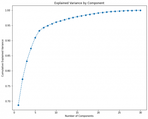
Figure 3. Components variances applying PCA using SMOTE
In addition, Figure 3's cumulative explained variance graph represents the amount of variation collected (along the y-axis) based on the number of components (features) included (the x-axis). A general rule is to retain between 80 and 90% of the volatility. Thus, in this instance, we decide to keep 8 features only. These features are: “scaled_amount”, “V1”, “V4”, “V8”, “V12”, “V14”, and “V21”.
Table 2 presents all the experiments done in Branch-2. Bagging, RF classifiers and the voting technique outperformed better accuracy in PCA branch's in first sub-part. The voting technique surpassed the others in the first sub-part (PCA/SMOTE). LR's resulted in lower missclassification rate for fraud (minority) class in first sub-part, and NB resulted in lower classification in second sub-part. However, both classifiers produced a higher misclassification rate for the non-fraud (majority) class than the RF. RF also performed the best in the second sub-part against other classifiers.
• Branch-3 focuses on Linear Discriminant Analysis (LDA) as a dimensionality reduction technique and SMOTE for oversampling. After several hit & trial experiments, we have feed LDA with one (1) component to perform all experiments in this branch. Table 3 summarizes all of the Branch-3 experiments. In both classes, the voting ensemble learning technique outperformed the first sub-part of (LDA) branch. NB outperformed in the second sub-part (LDA/SMOTE); However, LR resulted in a lower misclassification rate for the fraud (minority) class in first sub-part and Bagging, DT and RF resulted in second sub-part.
• Branch-4 focuses on autoencoder as the dimension reduction technique along with SMOTE as oversampling technique. In both sub-parts, the identical autoencoder design has been maintained. Typically, autoencoders are composed of two components: the encoder and the decoder. The bottleneck layer displays their compressed form between the input features and the bottleneck layer.
The encoder part consists of two blocks, each composed of 1D Convolution Neural Network (CNN) followed by 1D Max-Pooling. The decoder part consists of two blocks, each consisting of 1D Upsampling followed by 1D CNN. Table 4 presents all the experiments done in Branch-4. Bagging, DT, RF and AdaBoost classifiers outperformed in the first sub-part, and RF outperformed in the second sub-part. The Autoencoder branch does not have good accuracy because a complex network to compress the features has been chosen, and different optimizers and batch sizes to check the results have been tried in vain.
The primary objective of principle component analysis (PCA) is to minimize the dimensionality of the data containing multiple variables that are strongly or weakly associated with one another, while preserving the variation contained in the data set to the greatest extent possible. This is achieved by transforming the variables into a new set of variables, which is a set of properties or attributes from our original dataset, in such a way that the maximum variety is preserved.
Table 1. Results (Branch-1)
|
Classifier |
DR |
Oversampling |
TN |
FP |
FN |
TP |
Acc. |
Prec. |
Rec. |
F1-Score |
|
Bagging |
- |
- |
56861 |
03 |
21 |
77 |
100.0% |
96.3% |
78.6% |
86.5% |
|
DT |
56835 |
29 |
21 |
77 |
99.9% |
72.6% |
78.6% |
75.5% |
||
|
RF |
56862 |
02 |
24 |
74 |
100.0% |
97.4% |
75.5% |
85.1% |
||
|
AdaBoost |
56852 |
12 |
27 |
71 |
99.9% |
85.5% |
72.4% |
78.5% |
||
|
NB |
55619 |
1245 |
18 |
80 |
97.8% |
06.0% |
81.6% |
11.2% |
||
|
LR |
56855 |
09 |
43 |
55 |
99.9% |
85.9% |
56.1% |
67.9% |
||
|
SVM |
56862 |
02 |
33 |
65 |
99.9% |
97.0% |
66.3% |
78.8% |
||
|
MV |
56862 |
02 |
23 |
75 |
99.9% |
97.4% |
76.5% |
85.6% |
||
|
Bagging |
- |
SMOTE |
56824 |
40 |
18 |
80 |
99.9% |
66.7% |
81.6% |
73.4% |
|
DT |
56752 |
112 |
22 |
76 |
99.8% |
40.4% |
77.6% |
53,1% |
||
|
RF |
56856 |
08 |
16 |
82 |
100.0% |
91.1% |
83.7% |
87.2% |
||
|
AdaBoost |
55532 |
1332 |
06 |
92 |
97.7% |
06.5% |
93.9% |
12.1% |
||
|
NB |
55499 |
1365 |
13 |
85 |
97.6% |
05.9% |
86.7% |
11.0% |
||
|
LR |
55455 |
1409 |
08 |
90 |
97.5% |
06.0% |
91.8% |
11.3% |
||
|
SVM |
55980 |
884 |
12 |
86 |
98.4% |
08.9% |
87.8% |
16.1% |
||
|
MV |
56814 |
50 |
11 |
87 |
99.9% |
63.5% |
88.8% |
74.0% |
Table 2. Results (Branch-2)
|
Classifier |
DR |
Oversampling |
TN |
FP |
FN |
TP |
Acc. |
Prec. |
Rec. |
F1-Score |
|
Bagging |
PCA |
- |
56862 |
02 |
23 |
75 |
100.0% |
97.4% |
76.5% |
85.7% |
|
DT |
56843 |
21 |
24 |
74 |
99.9% |
77.9% |
75.5% |
76.7% |
||
|
RF |
56863 |
01 |
22 |
76 |
100.0% |
98.7% |
77.6% |
86.9% |
||
|
AdaBoost |
56849 |
15 |
27 |
71 |
99.9% |
82.6% |
72.4% |
77.2% |
||
|
NB |
55865 |
999 |
18 |
80 |
98.2% |
07.4% |
81.6% |
13.6% |
||
|
LR |
56855 |
09 |
41 |
57 |
99.9% |
86.4% |
58.2% |
69.5% |
||
|
SVM |
56862 |
02 |
33 |
65 |
99.9% |
97.0% |
66.3% |
78.8% |
||
|
MV |
56862 |
02 |
26 |
72 |
100.0% |
97.3% |
73.5% |
83.7% |
||
|
Bagging |
PCA |
SMOTE |
56757 |
107 |
16 |
82 |
99.8% |
43.4% |
83.7% |
57.1% |
|
DT |
56625 |
239 |
16 |
82 |
99.6% |
25.5% |
83.7% |
39.1% |
||
|
RF |
56803 |
61 |
12 |
86 |
99.9% |
58.5% |
87.8% |
70.2% |
||
|
AdaBoost |
54977 |
1887 |
9 |
89 |
96.7% |
04.5% |
90.8% |
8.6% |
||
|
NB |
54591 |
2273 |
14 |
84 |
96.0% |
03.6% |
85.7% |
6.8% |
||
|
LR |
55505 |
1359 |
8 |
90 |
97.6% |
06.2% |
91.8% |
11.6% |
||
|
SVM |
55982 |
882 |
10 |
88 |
98.4% |
09.1% |
89.8% |
16.5% |
||
|
MV |
56787 |
77 |
11 |
87 |
99.8% |
53.0% |
88.8% |
66.4% |
Table 3. Results (Branch-3)
|
Classifier |
DR |
Oversampling |
TN |
FP |
FN |
TP |
Acc. |
Prec. |
Rec. |
F1-Score |
|
Bagging |
LDA |
- |
56846 |
18 |
28 |
70 |
99.9% |
79.5% |
71.4% |
75.3% |
|
DT |
56841 |
23 |
28 |
70 |
99.9% |
75.3% |
71.4% |
73.3% |
||
|
RF |
56844 |
20 |
28 |
70 |
99.9% |
77.8% |
71.4% |
74.5% |
||
|
AdaBoost |
56851 |
13 |
22 |
76 |
99.9% |
85.4% |
77.6% |
81.3% |
||
|
NB |
56843 |
21 |
20 |
78 |
99.9% |
78.8% |
79.6% |
79.2% |
||
|
LR |
56854 |
10 |
42 |
56 |
99.9% |
84.8% |
57.1% |
68.3% |
||
|
SVM |
56852 |
12 |
22 |
76 |
99.9% |
86.4% |
77.6% |
81.7% |
||
|
MV |
56858 |
06 |
25 |
73 |
99.9% |
92.4% |
74.5% |
82.5% |
||
|
Bagging |
LDA |
SMOTE |
51750 |
5114 |
12 |
86 |
91.0% |
01.7% |
87.8% |
3.2% |
|
DT |
51124 |
5740 |
12 |
86 |
89.9% |
01.5% |
87.8% |
2.9% |
||
|
RF |
51101 |
5763 |
12 |
86 |
89.9% |
01.5% |
87.8% |
2.9% |
||
|
AdaBoost |
54498 |
2366 |
08 |
90 |
95.8% |
03.7% |
91.8% |
7.0% |
||
|
NB |
55296 |
1568 |
08 |
90 |
97.2% |
05.4% |
91.8% |
10.3% |
||
|
LR |
54575 |
2289 |
08 |
90 |
96.0% |
03.8% |
91.8% |
7.3% |
||
|
SVM |
55218 |
1646 |
08 |
90 |
97.1% |
05.2% |
91.8% |
9.8% |
||
|
MV |
54893 |
1971 |
08 |
90 |
96.5% |
04.4% |
91.8% |
8.3% |
Table 4. Results (Branch-4)
|
Classifier |
DR |
Oversampling |
TN |
FP |
FN |
TP |
Acc. |
Prec. |
Rec. |
F1-Score |
|
Bagging |
Autoencoder |
- |
56855 |
09 |
43 |
55 |
99.9% |
85.9% |
56.1% |
76.9% |
|
DT |
56834 |
30 |
46 |
52 |
99.9% |
63.4% |
53.1% |
57.8% |
||
|
RF |
56859 |
05 |
40 |
58 |
99.9% |
92.1% |
59.2% |
72.0% |
||
|
AdaBoost |
56844 |
20 |
58 |
40 |
99.9% |
66.7% |
40.8% |
50.6% |
||
|
NB |
56209 |
655 |
43 |
55 |
98.8% |
07.7% |
56.1% |
13.6% |
||
|
LR |
56856 |
8 |
81 |
17 |
99.8% |
68.0% |
17.3% |
27.6% |
||
|
SVM |
56864 |
0 |
89 |
9 |
99.8% |
100.0% |
09.2% |
16. 8% |
||
|
MV |
56862 |
02 |
53 |
45 |
99.9% |
95.7% |
45.9% |
62.1% |
||
|
Bagging |
Autoencoder |
SMOTE |
56141 |
723 |
49 |
49 |
98.6% |
6.3% |
50.0% |
11.3% |
|
DT |
55544 |
1320 |
47 |
51 |
97.6% |
3.7% |
52.0% |
6.9% |
||
|
RF |
56485 |
379 |
48 |
50 |
99.3% |
11.7% |
51.0% |
19.0% |
||
|
AdaBoost |
49636 |
7228 |
22 |
76 |
87.3% |
1.0% |
77.6% |
2.1% |
||
|
NB |
46062 |
10802 |
25 |
73 |
81.0% |
0.7% |
74.5% |
1.3% |
||
|
LR |
53873 |
2991 |
42 |
56 |
94.7% |
1.8% |
57.1% |
3.6% |
||
|
SVM |
55291 |
1573 |
42 |
56 |
97.2% |
3.4% |
57.1% |
6.5% |
||
|
MV |
56001 |
863 |
38 |
60 |
98.4% |
6.5% |
61.2% |
11.8% |
While The purpose of linear discriminant analysis (LDA) is to improve the separability between two groups so that we may make the best classification decision possible. Although both PCA and LDA contribute to dimensionality reduction, LDA focuses on optimizing the separability between known categories by generating a new linear axis and projecting the data points down that axis. LDA is not concerned with locating the primary component; rather, it examines which types of points/features/subspace provide the most discrimination for separating the data. LDA's purpose is to locate a line that optimizes class separation.
The autoencoder maps the input to the latent space, and the decoder reassembles the input. For correct reconstruction of the input, they are trained by back propagation. Dimensionality reduction can be achieved with autoencoders when the latent space has less dimensions than the input. Since they are capable of recreating the input, these low-dimensional latent variables should, intuitively, encode its most essential characteristics.
Autoencoders are able to model complex nonlinear functions, whereas PCA and LDA are essentially linear transformations. Since PCA features are projections on an orthogonal basis, they are completely linearly uncorrelated with one another. However, autoencoder features may have correlations because they were merely trained for correct reconstruction.
Both PCA and LDA attempt to minimize dimensions. PCA seeks out characteristics with the greatest variance. LDA attempts to optimize the separation between recognized categories. In addition, we can conduct that both of PCA and LDA are very comparable; both are linear transformation methods that use eigenvalues and eigenvectors to break up matrices. The major difference is that LDA requires class labels into account while PCA does not because it is not supervised.
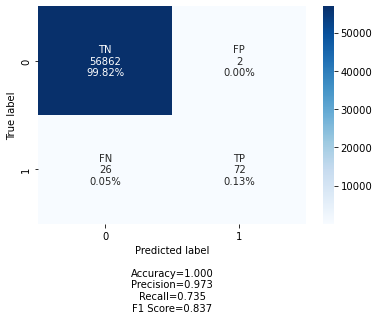
Overall Analysis provides insight into the results of all four (4) branches and mainly focuses on the Voting ensemble learning technique. Overall experiments showed that the best result came in Branch-2's first sub-part (PCA) with 100.0% accuracy, 97.3% precision, 73.5% recall, and 83.7% f1-score in both classes.
However, if the minority class (fraud) has been focused on, some experiments performed better but resulted in a higher misclassification rate for the majority class (non-fraud).
The confusion matrix was employed to conduct a detailed analysis of the best experiment. The confusion matrix is a technique for evaluating the effectiveness of ML algorithms when performing classification tasks. It functions in the same way as a table, assisting in explaining the model's performance on a test dataset. The term confusion matrix is very simple but its approach is little bit confusing. The basic purpose of confusion matrix is to visualize the accuracy of proposed classifier by comparing predicted and actual classes. The binary confusion is composed of squares. The following four terms are explained in greater detail by the confusion matrix.
• TP: Predicted values were correct when they turned out to be positive.
• FP: Forecasted values were wrongly predicted as positive when they were negative. Specifically, negative values are projected to be positive.
• FN: Positive values are expected to be negative.
• TN: Predicted values were properly predicted as negative in the actual data.
Figure 4. CM for the best performing model
Figure 4 depicts the confusion matrix for the overall best result produced from Branch-2, which is the most favorable outcome. FNs are limited to twenty six (26), while FPs are limited to two (2), as seen in the table. Our strategy was based on two research questions we had formulated in the first place and on which we sought answers. We will be able to answer the questions after completing all the experiments and analyses. The answer to the first question is Yes since voting ensemble learning employs majority voting to make the final prediction, and the answer is Yes. As a result, if the underlying models produce accurate forecasts, the vote will almost certainly improve the situation. Regarding the second question, the answer is also yes, because we concluded that PCA oversampling technique can give more reliable results than other oversampling techniques. We have only studied the SMOTE technique for oversampling, which is frequently used by researchers and is the only one we have tested.
The detection of fraudulent transactions has been happening for the past twenty years. The researchers have implemented various methods for efficient and timely detection of fraudulent activities. ML models have shown promising results in timely and accurate fraud detection, yet datasets have some limitations. Deep learning models provide better results in having a sufficient and accurate dataset for learning representations. This paper proposes an approach with a voting ensemble learning technique combined with ML classifiers. Various dimensionality reduction techniques have been used, including PCA, LDA, and Autoencoder. SMOTE has been used for oversampling of the dataset. As the number of instances increases, the proposed approach uses the good in every ML classifier to learn about the fraudulent dataset. The main goal of this paper is to determine fraudulent transaction activities by using different ML techniques. The best result has been obtained using the voting ML technique. Future works include using a dataset with more fraudulent transactions for the models to learn and perform better. Current datasets are imbalanced and contain more non-fraudulent transactions, making the model biased toward the majority class.
[1] Kou, Y., Lu, C.T., Sirwongwattana, S., Huang, Y.P. (2004). Survey of fraud detection techniques. In IEEE International Conference on Networking, Sensing and Control, Taipei, Taiwan, pp. 749-754. https://doi.org/10.1109/ICNSC.2004.1297040
[2] Turban, E., Sharda, R., Delen, D. (2001). Decision Support and Business Intelligence System. Prentice Hall, New Jersey.
[3] Awoyemi, J.O., Adetunmbi, A.O., Oluwadare, S.A. (2017). Credit card fraud detection using machine learning techniques: A comparative analysis. In 2017 International Conference on Computing Networking And Informatics (ICCNI), Lagos, Nigeria, pp. 1-9. https://doi.org/10.1109/ICCNI.2017.8123782
[4] Obermeyer, Z., Emanuel, E.J. (2016). Predicting the future—Big data, machine learning, and clinical medicine. The New England Journal of Medicine, 375(13): 1216. https://doi.org/10.1056/nejmp1606181
[5] Baker, M.R., Padmaja, D.L., Puviarasi, R., Mann, S., Panduro-Ramirez, J., Tiwari, M., Samori, I.A. (2022). Implementing critical machine learning (ML) approaches for generating robust discriminative neuroimaging representations using structural equation model (SEM). Computational and Mathematical Methods in Medicine. https://doi.org/10.1155/2022/6501975
[6] Li, F., Tang, H., Zou, Y., Huang, Y., Feng, Y., Peng, L. (2021). Research on information security in text emotional steganography based on machine learning. Enterprise Information Systems, 15(7): 984-1001. https://doi.org/10.1080/17517575.2020.1720827
[7] Gombolay, M.C., Jensen, R.E., Son, S.H. (2017). Machine learning techniques for analyzing training behavior in serious gaming. IEEE Transactions on Games, 11(2): 109-120. https://doi.org/10.1109/TCIAIG.2017.2754375
[8] Qader, B.A., Jihad, K.H., Baker, M.R. (2022). Evolving and training of neural network to play DAMA board game using NEAT algorithm. Informatica, 46(5): 29–37. https://doi.org/10.31449/inf.v46i5.3897
[9] Zimmermann-Niefield, A., Shapiro, R.B., Kane, S. (2019). Sports and machine learning: How young people can use data from their own bodies to learn about machine learning. XRDS: Crossroads, The ACM Magazine for Students, 25(4): 44-49. https://doi.org/10.1145/3331071
[10] Nooruldeen, O., Alturki, S., Baker, M.R., Ghareeb, A. (2022). Time series forecasting for decision making on city-wide energy demand: A comparative study. In 2022 International Conference on Decision Aid Sciences and Applications (DASA), pp. 1706-1710. https://doi.org/10.1109/DASA54658.2022.9765193
[11] Rundo, F., Trenta, F., di Stallo, A.L., Battiato, S. (2019). Machine learning for quantitative finance applications: A survey. Applied Sciences, 9(24): 5574. https://doi.org/10.3390/app9245574
[12] Jiang, C., Song, J., Liu, G., Zheng, L., Luan, W. (2018). Credit card fraud detection: A novel approach using aggregation strategy and feedback mechanism. IEEE Internet of Things Journal, 5(5): 3637-3647. https://doi.org/10.1109/JIOT.2018.2816007
[13] Bose, I., Mahapatra, R.K. (2001). Business data mining—a machine learning perspective. Information & Management, 39(3): 211-225. https://doi.org/10.1016/S0378-7206(01)00091-X
[14] Abdallah, A., Maarof, M.A., Zainal, A. (2016). Fraud detection system: A survey. Journal of Network and Computer Applications, 68: 90-113. https://doi.org/10.1016/j.jnca.2016.04.007
[15] Guo, T., Li, G.Y. (2008). Neural data mining for credit card fraud detection. In 2008 International Conference on Machine Learning and Cybernetics, pp. 3630-3634.
[16] Asha, R.B., Suresh Kumar, K.R. (2021). Credit card fraud detection using artificial neural network. Global Transitions Proceedings, 2(1): 35-41. https://doi.org/10.1016/j.gltp.2021.01.006
[17] Sparrow, M.K., Chiles, L. (2019). License to Steal: Why Fraud Plagues America’s Health Care System. Routledge, New York. https://doi.org/10.4324/9780429039577
[18] Wen, C.H., Wang, M.J., Lan, L.W. (2005). Discrete choice modeling for bundled automobile insurance policies. Journal of the Eastern Asia Society for Transportation Studies, 6: 1914-1928. https://doi.org/10.11175/easts.6.1914
[19] Chang, W.H., Chang, J.S. (2012). An effective early fraud detection method for online auctions. Electronic Commerce Research and Applications, 11(4): 346-360. https://doi.org/10.1016/j.elerap.2012.02.005
[20] Fu, K., Cheng, D., Tu, Y., Zhang, L. (2016). Credit card fraud detection using convolutional neural networks. In International Conference on Neural Information Processing, pp. 483-490. https://doi.org/10.1007/978-3-319-46675-0_53
[21] Cody, T., Adams, S., Beling, P.A. (2018). A utilitarian approach to adversarial learning in credit card fraud detection. In 2018 Systems and Information Engineering Design Symposium (SIEDS), Charlottesville, VA, USA, pp. 237-242. https://doi.org/10.1109/SIEDS.2018.8374743
[22] Hines, C., Youssef, A. (2018). Machine learning applied to rotating check fraud detection. In 2018 1st International Conference on Data Intelligence and Security (ICDIS), South Padre Island, TX, USA, pp. 32-35. https://doi.org/10.1109/ICDIS.2018.00012
[23] Lucas, Y., Portier, P.E., Laporte, L., He-Guelton, L., Caelen, O., Granitzer, M., Calabretto, S. (2020). Towards automated feature engineering for credit card fraud detection using multi-perspective HMMs. Future Generation Computer Systems, 102: 393-402. https://doi.org/10.1016/j.future.2019.08.029
[24] Pumsirirat, A., Liu, Y. (2018). Credit card fraud detection using deep learning based on auto-encoder and restricted boltzmann machine. International Journal of Advanced Computer Science and Applications, 9(1): 18–25. https://doi.org/10.14569/IJACSA.2018.090103
[25] Gao, J., Gong, L., Wang, J.Y., Mo, Z.C. (2018). Study on unbalanced binary classification with unknown misclassification costs. In 2018 IEEE International Conference on Industrial Engineering and Engineering Management (IEEM), Bangkok, Thailand, pp. 1538-154. https://doi.org/10.1109/IEEM.2018.8607671
[26] Mathew, J., Pang, C.K., Luo, M., Leong, W.H. (2017). Classification of imbalanced data by oversampling in kernel space of support vector machines. IEEE Transactions on Neural Networks and Learning Systems, 29(9): 4065-4076. https://doi.org/10.1109/TNNLS.2017.2751612
[27] Hormozi, H., Akbari, M.K., Hormozi, E., Javan, M.S. (2013). Credit cards fraud detection by negative selection algorithm on hadoop (To reduce the training time). In The 5th Conference on Information and Knowledge Technology, Shiraz, Iran, pp. 40-43. https://doi.org/10.1109/IKT.2013.6620035
[28] Quah, J.T.S., Sriganesh, M. (2008). Real-time credit card fraud detection using computational intelligence. Expert Systems with Applications, 35(4): 1721–1732. https://doi.org/10.1016/j.eswa.2007.08.093
[29] Kundu, A., Panigrahi, S., Sural, S., Majumdar, A.K. (2009). BLAST-SSAHA hybridization for credit card fraud detection. IEEE Transactions on Dependable and Secure Computing, 6(4): 309–315. https://doi.org/10.1109/TDSC.2009.11
[30] Wang, L., Liu, T., Wang, G., Chan, K.L., Yang, Q. (2015). Video tracking using learned hierarchical features. IEEE Transactions on Image Processing, 24(4): 1424–1435. https://doi.org/10.1109/TIP.2015.2403231
[31] Jurgovsky, J., Granitzer, M., Ziegler, K., Calabretto, S., Portier, P.E., He-Guelton, L., Caelen, O. (2018). Sequence classification for credit-card fraud detection. Expert Systems with Applications, 100: 234-245. https://doi.org/10.1016/j.eswa.2018.01.037
[32] Fiore, U., De Santis, A., Perla, F., Zanetti, P., Palmieri, F. (2019). Using generative adversarial networks for improving classification effectiveness in credit card fraud detection. Information Sciences, 479: 448–455. https://doi.org/10.1016/j.ins.2017.12.030
[33] Carcillo, F., Le Borgne, Y.A., Caelen, O., Kessaci, Y., Oblé, F., Bontempi, G. (2021). Combining unsupervised and supervised learning in credit card fraud detection. Information Sciences, 557: 317–331. https://doi.org/10.1016/j.ins.2019.05.042
[34] Carcillo, F., Dal Pozzolo, A., Le Borgne, Y.A., Caelen, O., Mazzer, Y., Bontempi, G. (2018). SCARFF: A scalable framework for streaming credit card fraud detection with spark. Information Fusion, 41: 182–194. https://doi.org/10.1016/j.inffus.2017.09.005
[35] Saia, R., Carta, S. (2017). A frequency-domain-based pattern mining for credit card fraud detection. IoTBDS 2017 - Proceedings of the 2nd International Conference on Internet of Things, Big Data and Security, Porto, pp. 386–391.
[36] Rtayli, N., Enneya, N. (2020). Enhanced credit card fraud detection based on SVM-recursive feature elimination and hyper-parameters optimization. Journal of Information Security and Applications, 55: 102596. https://doi.org/10.1016/j.jisa.2020.102596
[37] Zhang, X., Han, Y., Xu, W., Wang, Q. (2021). HOBA: A novel feature engineering methodology for credit card fraud detection with a deep learning architecture. Information Sciences, 557: 302–316. https://doi.org/10.1016/j.ins.2019.05.023
[38] Cao, P., Liu, X., Zhang, J., Zhao, D., Huang, M., Zaiane, O. (2017). ℓ2,1 norm regularized multi-kernel based joint nonlinear feature selection and over-sampling for imbalanced data classification. Neurocomputing, 234: 38–57. https://doi.org/10.1016/j.neucom.2016.12.036
[39] Zhang, F., Liu, G., Li, Z., Yan, C., Jiang, C. (2019). GMM-based undersampling and its application for credit card fraud detection. Proceedings of the International Joint Conference on Neural Networks, Budapest, pp. 1–8.
[40] Thabtah, F., Hammoud, S., Kamalov, F., Gonsalves, A. (2020). Data imbalance in classification: Experimental evaluation. Information Sciences, 513: 429–441. https://doi.org/10.1016/j.ins.2019.11.004
[41] Makki, S., Assaghir, Z., Taher, Y., Haque, R., Hacid, M.S., Zeineddine, H. (2019). An experimental study with imbalanced classification approaches for credit card fraud detection. IEEE Access, 7: 93010-93022. https://doi.org/10.1109/ACCESS.2019.2927266
[42] Sohony, I., Pratap, R., Nambiar, U. (2018). Ensemble learning for credit card fraud detection. ACM International Conference Proceeding Series, Goa, pp. 289–294.
[43] Chawla, N.V., Bowyer, K.W., Hall, L.O., Kegelmeyer, W.P. (2002). SMOTE: Synthetic minority over-sampling technique. Journal of Artificial Intelligence Research, 16: 321–357. https://doi.org/10.1613/jair.953
[44] Peng, C.Y.J., Lee, K.L., Ingersoll, G.M. (2002). An introduction to logistic regression analysis and reporting. Journal of Educational Research, 96(1): 3–14. https://doi.org/10.1080/00220670209598786
[45] Itoo, F., Singh, S. (2021). Comparison and analysis of logistic regression, Naïve Bayes and KNN machine learning algorithms for credit card fraud detection. International Journal of Information Technology, 13(4): 1503-1511. https://doi.org/10.1007/s41870-020-00430-y
[46] Midi, H., Sarkar, S.K., Rana, S. (2010). Collinearity diagnostics of binary logistic regression model. Journal of Interdisciplinary Mathematics, 13(3): 253–267. https://doi.org/10.1080/09720502.2010.1070069
[47] Cervantes, J., Garcia-Lamont, F., Rodríguez-Mazahua, L., Lopez, A. (2020). A comprehensive survey on support vector machine classification: Applications, challenges and trends. Neurocomputing, 408: 189–215. https://doi.org/10.1016/j.neucom.2019.10.118
[48] Trafalis, T.B., Ince, H. (2000). Support vector machine for regression and applications to financial forecasting. Proceedings of the International Joint Conference on Neural Networks, pp. 348–353.
[49] Xu, M., Watanachaturaporn, P., Varshney, P.K., Arora, M.K. (2005). Decision tree regression for soft classification of remote sensing data. Remote Sensing of Environment, 97(3): 322–336. https://doi.org/10.1016/j.rse.2005.05.008
[50] Kotsiantis, S.B. (2013). Decision trees: A recent overview. Artificial Intelligence Review, 39(4): 261–283. https://doi.org/10.1007/s10462-011-9272-4
[51] Rustam, F., Mehmood, A., Ullah, S., Ahmad, M., Muhammad Khan, D., Choi, G.S., On, B.W. (2020). Predicting pulsar stars using a random tree boosting voting classifier (RTB-VC). Astronomy and Computing, 32: 100404. https://doi.org/10.1016/j.ascom.2020.100404
[52] Rashidi, S., Ranjitkar, P. (2015). Estimation of bus dwell time using univariate time series models. Journal of Advanced Transportation, 49(1): 139–152. https://doi.org/10.1002/atr.1271
[53] Alzubaidi, L., Zhang, J., Humaidi, A.J., Al-Dujaili, A., Duan, Y., Al-Shamma, O., Santamaría, J., Fadhel, M.A., Al-Amidie, M., Farhan, L. (2021). Review of deep learning: Concepts, CNN architectures, challenges, applications, future directions. Journal of Big Data, 8(1): 1–74. https://doi.org/10.1186/s40537-021-00444-8
[54] Xu, Z., Li, C., Yang, Y. (2021). Fault diagnosis of rolling bearings using an improved multi-scale convolutional neural network with feature attention mechanism. ISA Transactions, 110: 379–393. https://doi.org/10.1016/j.isatra.2020.10.054
[55] Shahraki, A., Abbasi, M., Haugen, Ø. (2020). Boosting algorithms for network intrusion detection: A comparative evaluation of real Adaboost, gentle Adaboost and modest Adaboost. Engineering Applications of Artificial Intelligence, 94: 103770. https://doi.org/10.1016/j.engappai.2020.103770
[56] Soria, D., Garibaldi, J.M., Ambrogi, F., Biganzoli, E.M., Ellis, I.O. (2011). A “Non-parametric” version of the naive bayes classifier. Knowledge-Based Systems, 24(6): 775–784. https://doi.org/10.1016/j.knosys.2011.02.014
[57] Nti, I.K., Adekoya, A.F., Weyori, B.A. (2020). A comprehensive evaluation of ensemble learning for stock-market prediction. Journal of Big Data, 7(1): 1–40. https://doi.org/10.1186/s40537-020-00299-5
[58] Peppes, N., Daskalakis, E., Alexakis, T., Adamopoulou, E., Demestichas, K. (2021). Performance of machine learning-based multi-model voting ensemble methods for network threat detection in agriculture 4.0. Sensors, 21(22): 7475. https://doi.org/10.3390/s21227475