Habib Mohammed* | Adil Tannouche | Youssef Ounejjar
© 2022 IIETA. This article is published by IIETA and is licensed under the CC BY 4.0 license (http://creativecommons.org/licenses/by/4.0/).
OPEN ACCESS
The fight against weed remains one of the major challenges in agriculture to improve land productivity. The first and most important step of this fight is to detect and locate this weed. Artificial intelligence has played a very important contribution in this detection. Several applications have been developed using Deep Learning techniques to detect and identify weed, but the variety of weed types complicates this operation. We propose a Deep Learning technique to detect and localize the crop, by training the pretrained Faster RCNN ResNet model with a rich dataset. We developed an algorithm able to detect and ultra-localize the pea crop with a prediction up to 100%. The obtained results show the feasibility of this method to distinguish the crop among weed.
computer vision, deep learning, weed detection, precision agriculture, pea cultivation
The fight against weed is part of the daily life of farmers, because it affects their productivity. To achieve this fight, the use of chemical treatments is necessary. The Artificial intelligence, and more precisely Deep Learning, can help to identify or detect precisely the location of this weed, which can help to limit the use of chemical products by treating only the areas concerned.
The works that have been realized in our research team has made it possible to optimize the use of chemical treatments, through the automatic control of sprayers according to the location of weed, with the objective of preserving the environment and limiting the use of herbicides, using artificial intelligence techniques. These works were based, in the first place, on the combination of Haar's pseudo-features with the Ada Boost algorithm, to detect weed of different crops in real time [1]. In the same framework, another work has developed a new adjacency descriptor for weed selection in real time for sprayer control [2].
In the context of organic agriculture, which excludes the use of chemical treatments [3-5], weed control is based on the practice of manual weeding, which is a tiring operation that requires the presence of humans in the fields [6, 7]. In the perspective of dehumanising this procedure and to explore the agriculture 4.0 [8-12], we have a vision of realising an automated mechanical system, based on Deep Learning [13], able to simulate manual weed removal by mechanical, thermal or chemical destruction of the weed by targeting only itself. Here appears the necessity to have a new method of detection and ultra-localization of weed.
Using convolutional neural networks, and more precisely object detectors such as the SSD model [14], Faster RCNN [15], the ResNet [16], the CenterNet [17] etc., several researches have been elaborated in order to distinguish between crops and weeds [18, 19]. These studies have not been able to make the ultra-localization because they were based on aerial images, which can be obtained if we take images in a few centimeters of the earth.
The objective of this study is to develop an algorithm based on Deep Learning, by training the Faster RCNN ResNet pretrained model, to detect and ultra-locate the crop among weed with a very high accuracy.
Our method consists of fine-tuning the predefined Faster RCNN ResNet model, with a collected and pre-treated DataSet and augmented to generate a neural network that can detect and locate the crop and draw a bounding box around it and associate its prediction percentage, i.e. discriminate the plant from the weed.
We chose to work with the Faster RCNN ResNet 50 model which is one of the most popular models, it is a fast model (89 ms), its accuracy is 30 COCO mAP and it is able to generate bounding boxes around the objects.
2.1 Acquisition and images annotations
The selected plant is the pea (JELBANA in Arabic), we chose it because it is a crop that is fragile and more sensitive to weed, and it is more popular in the study area.
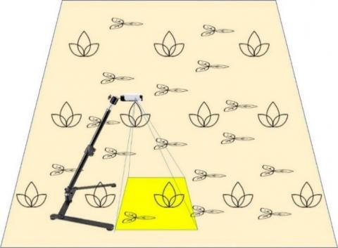
The images of this plant were collected using a digital camera phone (Huawei Y7 prime), the crop was planted in a field located in the city of MEKNES in MOROCCO (N33°52’37.647" & O5°34'4.25"). The images are captured using the devices shown in Figure 1.
Figure 1. Image acquisition devices (at about 40cm from the soil)
The original dimensions of the images are 3120x4160 pixels, they are taken in different types of parcels of land and different times of the day. Subsequently they are resized to the working size of 780x1040 pixels using the image processing functionalities of the OpenCv and Python libraries, for reasons of acceptable size for the model and the limitation of storing the data in Google Drive. The samples of the captured images are shown in Figure 2.
Figure 2. The basic samples of image data
The annotations of the images (or labelling) were done manually with the LabelImg software, which allows to draw the bounding box around the plants and exports an xml file containing the coordinates (xmin, xmax, ymin, ymax) of each bounding box as well as the object class and the name of the image that contains it.
2.2 DataSet augmentation
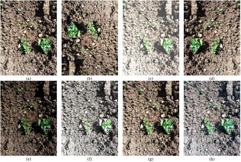
The training data contains 1156 images, and to enrich the DataSet, we proceeded to increase the data, using image processing methods with the Python OpenCv library. From a single image we generated 8 different images, 180° rotation, brightness increases and decreases, horizontal mirroring, contrast enhancement, Gaussian noise and histogram equalization. With these methods we obtained 9248 images as it shows the Figure 3.
2.3 The Faster R-CNN ResNet 50 model
The R-CNN is a convolutional neural network based on selective search to extract about 2000 regions called region proposals from the image. It allows to reduce the number of locations taken into account considerably. The application of this method solved the CNN localisation problem, but it was still too slow. It takes almost 50 seconds of testing per image [20].
Faster R-CNN was introduced to solve the problem of slow image processing speed, it is composed of Deep CNN to propose regions and Fast R-CNN to use the proposed regions. Faster R-CNN is quite faster than other models because it uses the method of selective search. A region proposal network (RPN) mainly tells the R-CNN where to search exactly. the Figure 4 shows the architecture of RCNN model
A single CNN takes the entire image as input and produces a feature map. On the feature map, RPN generates a set of proposed rectangles with objectivity scores as output. These values are then resized using RoI pooling to predict classes and bounding box regression. Figure 5 gives an idea of the functioning concept of the model.
Figure 3. (a) An original image augmented 8 ways using: (b) 180° rotation; (c) brightness increase; (d) horizontal mirror; (e) brightness decrease; (f) contrast enhancement; (g) gaussian noise; (h) histogram equalization
Figure 4. R-CNN model architecture
Figure 5. Structure of the Faster R-CNN model [21]
ResNet is an abbreviation for a residual network, as Deep Learning reaches its limits Microsoft had proposed a method to overcome the problem, which is the use of ResNet.
It consists of predicting results not only based on stacked layers, but also based on shortened connections that can skip one or more layers as shown in the example of the Figure 6.
Figure 6. A comparative example of a network with ResNet (b) and a network without ResNet (a)
For the 50-layer ResNet each 2-layers block is replaced in the 34-layers network by this 3-layers block, giving a 50-layers ResNet.
For the ResNet advantage, its results converge faster than its ordinary network.
For this research we adopted the Faster RCNN ResNet 50 model to detect the crop, it combines the functionalities of the two models which were already mentioned (Faster RCNN and ResNet 50).
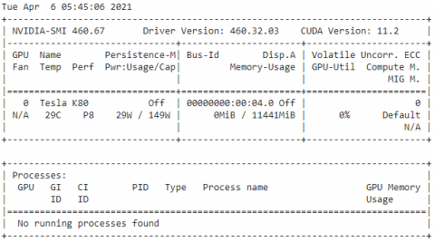
The platform we chose for the creation and training of our model is "Google Colab"[22], it is based on the Python language, as well as being configured with the essential machine learning and artificial intelligence libraries, such as TensorFlow, Matplotlib, and Keras. It is also possible to save and import files from google Drive, and most importantly it allows the use of GPU processor [23].
We took this opportunity to speed up and to perfect the learning of our model.
In order to make the reading of the data quicker, we opted to import our data on Google Drive. The characteristics of the training equipment is shown in Figure 7.
Figure 7. The processor performances and characteristics that we used for the training
The code we created allows us to read the data stored in Google Drive, 80% of the data is used for training and 20% for validation. The code converts the xml annotations to a csv file which compiles all these annotations in a table format and then creates a TFRecord file which allows the serialization/deserialization of the data, this is a format highly recommended by TensorFlow as it uses less space to hold a large amount of data.
The pre-trained model was downloaded from the TensorFlow 1 Detection Model Zoo open-source platform, with the configuration file [24].
We have modified the configurations in order to obtain better results, the initial configurations are mentioned in the Table 1.
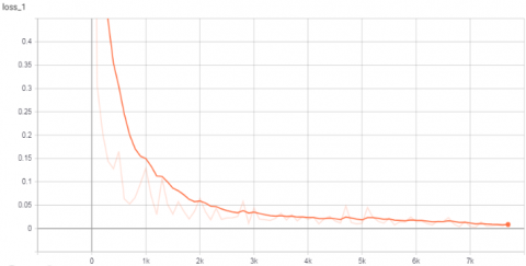
The training was started with a loss = 1.54, the training time in each 100 steps is almost 70 seconds, with a learning speed of 1.42 steps/sec almost stable throughout the training process:
When arriving at very advanced stages we notice that the error decreases a lot (Figure 8), it stabilizes around values lower than 0.05 which means a good learning.
Figure 8. The training loss plot (The real curve is the transparent curve and the other is the approximate curve)
Table 1. The model training configurations
|
Num classes |
Batch size |
Optimizer |
Initial learning rate |
Momentum |
Num steps |
Iou threshold |
|
1 |
4 |
Momentum optimizer |
0.0003 |
0.9 |
20000 |
0.50 |
To measure the accuracy of our model during training, we used the mAP (mean Average Precision) index, which is a metric used to measure the accuracy of object detectors such as Faster R-CNN, SSD, etc. [25]. The general definition of mean average precision (AP) is:
$A P=\int_{0}^{1} p(r)$ (1)
With p the precision and r the recall, these two parameters are defined by Goutte and Gaussier [26]:
$p=\frac{T P}{T P+F P}$ (2)
$r=\frac{T P}{T P+F N}$ (3)
TP: True Negative
TN: True Positive
FP: False Positive
FN: False Negative
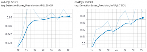
Using the Tensor Board tool, we plotted the accuracy traces of our model for the evaluation data (Figure 9), the model evaluation is done at every 50 steps:
Figure 9. mAP accuracy traces during training process (The real curve is the transparent curve and the other is the approximate curve)
The results change depending on the IoU threshold [27], for a threshold of IoU=0.75 the evaluation accuracy is limited to around 55%, and with a threshold of IoU=0.5 the evaluation accuracy stabilizes around 85%, that's why we chose a threshold of IoU=0.5.
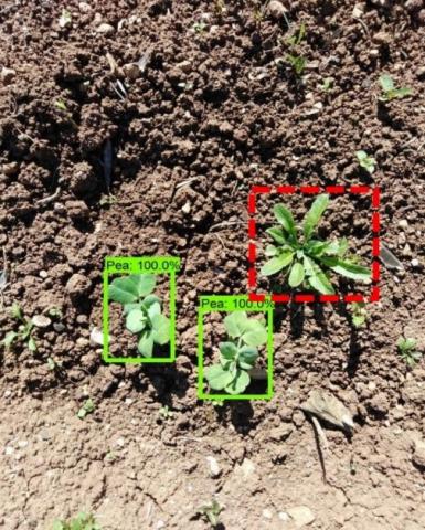
At the end of the training, we tested the model generated by the test images with different conditions (Figures 10 and 11).
Figure 10. Detection and ultra-localization of the culture under different conditions
Figure 11. Detection of pea in the presence of a weed (red box)
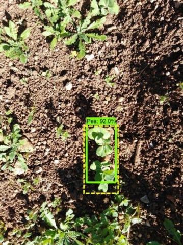
Figure 12. The yellow box indicates the desired result
Looking at the results obtained, it can be seen that the choice of a lower IoU threshold caused small errors in the bounding box occlusion of the whole crop (Figure 12), but this error does not affect the location of the plants, and can be resolved by enriching DataSet.
So, the trained model can identify and ultra-locate the crop with high predictions.
As we have previously mentioned, the variety of weed types has led us to the idea of crop detection alone which will help us to locate the weed as long as they are the rest of the weed that make up the image. This is a simpler method compared to the detection and classification of all weed types.
We have succeeded in building an algorithm based on Deep Learning that is able to detect and identify the pea plant among the weed. The algorithm is created from the pre-trained Faster RCNN ResNet model trained with images collected, pre-processed, annotated and increased. The obtained results are satisfactory enough, the trained model detects the crop with very high prediction reaching 100%.
The great variety of weed species complicates the detection process directly in images, because the model training requires a very rich database that contains all the weed variants, the absence of one type will cause the error of identification of this weed, so the idea of detecting the crop alone is more efficient and easier to implement.
The algorithm we have created highly supports our vision of an automatic weed control system for organic agriculture, and the results obtained show the feasibility of this system.
[1] Tannouche, A., Sbai, K., Rahmoune, M., Agounoune, R., Rahmani, A., Rahmani, A. (2016). Real time weed detection using a boosted cascade of simple features. International Journal of Electrical & Computer Engineering, 6(6): 2755-2765. https://doi.org/10.11591/ijece.v6i6.11878
[2] Tannouche, A., Sbai, K., Rahmoune, M., Zoubir, A., Agounoune, R., Saadani, R., Rahmani, A. (2016). A fast and efficient shape descriptor for an advanced weed type classification approach. International Journal of Electrical and Computer Engineering, 6(3): 1168-1175. https://doi.org/10.11591/ijece.v6i3.9978
[3] De Ponti, T., Rijk, B., van Ittersum, M. K. (2012). The crop yield gap between organic and conventional agriculture. Agricultural Systems, 108: 1-9. https://doi.org/10.1016/j.agsy.2011.12.004
[4] Gabriel, D., Sait, S.M., Kunin, W.E., Benton, T.G. (2013). Food production vs. biodiversity: comparing organic and conventional agriculture. Journal of Applied Ecology, 50(2): 355-364. https://doi.org/10.1111/1365-2664.12035
[5] Alonso, A.M., Guzmán, G.J. (2010). Comparison of the efficiency and use of energy in organic and conventional farming in Spanish agricultural systems. Journal of Sustainable Agriculture, 34(3): 312-338. https://doi.org/10.1080/10440041003613362
[6] Ramahi, A.A., Fathallah, F.A. (2006). Ergonomic evaluation of manual weeding practice and development of an ergonomic solution. Proceedings of the Human Factors and Ergonomics Society Annual Meeting, 50(13): 1421-1425. https://doi.org/10.1177/154193120605001335
[7] Melander, B., Rasmussen, G. (2001). Effects of cultural methods and physical weed control on intrarow weed numbers, manual weeding and marketable yield in direct-sown leek and bulb onion. Weed Research, 41(6): 491-508. https://doi.org/10.1046/j.1365-3180.2001.00252.x
[8] Zhai, Z., Martínez, J.F., Beltran, V., Martínez, N.L. (2020). Decision support systems for agriculture 4.0: Survey and challenges. Computers and Electronics in Agriculture, 170: 105256. https://doi.org/10.1016/j.compag.2020.105256
[9] Rose, D.C., Chilvers, J. (2018). Agriculture 4.0: Broadening responsible innovation in an era of smart farming. Frontiers in Sustainable Food Systems, 2: 87. https://doi.org/10.3389/fsufs.2018.00087
[10] Blackmore, S., Stout, B., Wang, M., Runov, B. (2005). Robotic agriculture–The future of agricultural mechanisation. In Proceedings of the 5th European Conference on Precision Agriculture, pp. 621-628. https://doi.org/10.3920/978-90-8686-549-9
[11] Duckett, T., Pearson, S., Blackmore, S., et al. (2018). Agricultural robotics: The future of robotic agriculture. arXiv preprint arXiv:1806.06762.
[12] Blackmore, S. (2016). Towards robotic agriculture. In Autonomous Air and Ground Sensing Systems for Agricultural Optimization and Phenotyping, 9866: 8-15. https://doi.org/10.1117/12.2234051
[13] Dimitriadis, S., Goumopoulos, C. (2008). Applying machine learning to extract new knowledge in precision agriculture applications. In 2008 Panhellenic Conference on Informatics, pp. 100-104. https://doi.org/10.1109/PCI.2008.30
[14] Liu, W., Anguelov, D., Erhan, D., Szegedy, C., Reed, S., Fu, C.Y., Berg, A.C. (2016). SSD: Single shot multibox detector. In European Conference on Computer Vision, pp. 21-37. https://doi.org/10.1007/978-3-319-46448-0_2
[15] Ren, S., He, K., Girshick, R., Sun, J. (2017). Faster R-CNN: Towards real-time object detection with region proposal networks. IEEE Trans Pattern Anal Mach Intell., 39(6): 1137-1149. https://doi.org/10.1109/TPAMI.2016.2577031
[16] He, K., Zhang, X., Ren, S., Sun, J. (2016). Deep residual learning for image recognition. In Proceedings of the IEEE Conference on Computer Vision and Pattern Recognition, pp. 770-778.
[17] Duan, K., Bai, S., Xie, L., Qi, H., Huang, Q., Tian, Q. (2019). Centernet: Keypoint triplets for object detection. In Proceedings of the IEEE/CVF International Conference on Computer Vision, pp. 6569-6578. https://doi.org/10.1109/iccv.2019.00667
[18] Dos Santos Ferreira, A., Matte Freitas, D., Gonçalves da Silva, G., Pistori, H., Theophilo Folhes, M. (2017). Weed detection in soybean crops using ConvNets. Computers and Electronics in Agriculture, 143: 314-324. https://doi.org/10.1016/j.compag.2017.10.027
[19] Kamilaris, A., Prenafeta-Boldú, F. (2018). A review of the use of convolutional neural networks in agriculture. The Journal of Agricultural Science, 156(3): 312-322. https://doi.org/10.1017/S0021859618000436
[20] Girshick, R., Donahue, J., Darrell, T., Malik, J. (2014). Rich feature hierarchies for accurate object detection and semantic segmentation. In Proceedings of the IEEE Conference on Computer Vision and Pattern Recognition, pp. 580-587. https://doi.org/10.1109/CVPR.2014.81
[21] Chen, Y., Li, W., Sakaridis, C., Dai, D., Van Gool, L. (2018). Domain adaptive faster R-CNN for object detection in the wild. In Proceedings of the IEEE Conference on Computer Vision and Pattern Recognition, pp. 3339-3348. https://doi.org/10.1109/CVPR.2018.00352
[22] Bisong, E. (2019). Building machine learning and deep learning models on Google cloud platform, Berkeley, CA, USA: Apress. pp. 59-64. https://doi.org/10.1007/978-1-4842-4470-8
[23] Carneiro, T., Da Nóbrega, R.V.M., Nepomuceno, T., Bian, G.B., De Albuquerque, V.H.C., Reboucas Filho, P. P. (2018). Performance analysis of google colaboratory as a tool for accelerating deep learning applications. IEEE Access, 6: 61677-61685. https://doi.org/10.1109/ACCESS.2018.2874767
[24] Rathod, V., Wu, N. (2017). TensorFlow detection model zoo (documentation). https://github.com/tensorflow/models/blob/master/research/object_detection/g3doc/tf1_detection_zoo.
[25] Henderson, P., Ferrari, V. (2016). End-to-end training of object class detectors for mean average precision. In Asian Conference on Computer Vision, pp. 198-213. https://doi.org/10.1007/978-3-319-54193-8_13
[26] Goutte, C., Gaussier, E. (2005). A probabilistic interpretation of precision recall and F-Score, with Implication for Evaluation. Advances in Information Retrieval, pp. 345-359. https://doi.org/10.1007/978-3-540-31865-1_25
[27] Rezatofighi, H., Tsoi, N., Gwak, J., Sadeghian, A., Reid, I., Savarese, S. (2019). Generalized intersection over union: A metric and a loss for bounding box regression. In Proceedings of the IEEE/CVF Conference on Computer Vision and Pattern Recognition, pp. 658-666. https://doi.org/10.1109/CVPR.2019.00075