Moussa Semchedine* | Noor Bensoula
© 2022 IIETA. This article is published by IIETA and is licensed under the CC BY 4.0 license (http://creativecommons.org/licenses/by/4.0/).
OPEN ACCESS
Black widow optimization algorithm is a recently evolutionary metaheuristic that imitates the unique mating behaviour of the black widow spiders in the real life. The trend of published papers utilizing the BWO algorithm is growing rapidly due to its efficiency in solving various engineering optimization problems. However, the BWO does not always perform as well as it should, and this is due to the random initialization of the spiders also the loss of good candidate solutions during the search. To remedy these problems, we propose in this paper a modified black widow optimization algorithm (MBWO) based on three ideas. First, an efficient initialization technique is adopted, which can guarantee starting the search with finest quality spiders and plays a significant role in determining an optimal or near-optimal solution. Second, the sexual cannibalism phase is modified to avoid the loss of high-quality solutions. Finally, an adaptive adjustment of crossover and mutation probabilities is presented to achieve a compromise between the diversification and intensification. Experiments are carried out on nineteen standard benchmark functions with different dimensions. The simulation results reveal that MBWO algorithm outperforms the original one also other metaheuristic algorithms in term of solution accuracy, global optimality, and the convergence speed.
black widow optimization algorithm, diversification, intensification, benchmark functions, evolutionary algorithms
Over the last decade, optimization theory and methods have grown rapidly and widely been applied in different engineering fields [1]. The complexity of the real-world optimization problems increases so that optimization algorithms especially those that are inspired from nature have received growing attention regarding their efficiency potential and ability to give the desired results [2].
Evolutionary algorithms are biologically inspired population-based approaches that mimic the Darwinian evolutionary in nature. Although, such efforts date back to the 1950s, so far, they have become popular tools for search, machine learning, and design problems [3]. These algorithms employ simulated evolution such as selection and procreation to find solutions for complicated problems. Within this paradigm achieving the best solution is seen as a survival duty, where all the possible solutions compete with each other to survive and this competition is the power of the evolutionary algorithms [4]. Several evolutionary algorithms have been proposed in the literature, historically the first proposition was the Genetic Algorithms (GAs) [5] then the Evolutionary strategies (ES) [6], Evolutionary programming (EP) [7] and Differential Evolution (DE) [8] popped out, the proposed approaches did not stop here, in the early nineties researchers have proposed other EAs, Genetic programming (GP) [9], Evolutionary Computation (EC) [10], Neuroevolution Algorithms (NAs) [11], etc. A brief review on the evolutionary algorithms can be found in research [12].
The Black Widow Optimization algorithm (BWO) is a recent metaheuristic, proposed by Hayyolalam and Kazem [13], inspired from the black spider’s unique behaviour mating. The working principle of this evolutionary algorithm is the same as that of the genetic algorithms (GAs) in procreation and mutation processes, however the mating of spiders involves an exclusive stage known as cannibalism, where the female black widow consumes its husband and the children consume each other and sometimes they consume their mother, due to this stage, individuals with insufficient fitness are excluded from the competition.
The trend of published papers utilizing BWO algorithm is growing rapidly. Houssein et al. [14] have proposed a novel Black Widow Optimization Algorithm for Multilevel Thresh-olding image segmentation named BWO-MT. The proposed algorithm is about to explore the search space for the aim of finding the optimal configuration of thresholds that maximize the Otsu’s and Kapur’s method using the crossover mutation and cannibalism operators, in which the widow is encoded a set of thresholds and tested each generation using Otsu or Kapur fitness functions. The BWO-MT was tested on a set of images with different degrees of complexity, and compared with six metaheuristics in which the results of the novel algorithm were the best in all metrics. However, when the Kapur’s entropy is used, the BWO’s fitness values are not the best. This fact occurs due to the randomness of the algorithm. Nanjappan et al. [15] presented an adaptive neuro fuzzy inference system and Black Widow Optimization approach (ANFIS-BWO) for optimal resource utilization and task scheduling in a cloud environment. The aim of the algorithm is to minimize computational time, cost, and energy consumptions of the tasks with useful resource utilization. Kumar [16] have developed an Energy Efficient Black Widow Optimization based Scheduling algorithm (EEBWOSA), for solving the problem of the increased demand of services of cloud computing that leads to increase in demand of energy consumption by data-center, and this by minimizing the consumption of power, energy costs and rising the profit. Micev et al. [17] proposed a hybrid method for identification of synchronous generator parameters using an adaptive BWO algorithm, where the aim was to minimize the normalized sum of squared errors (NSSE) between simulation and experimental results. The proposed algorithm ensures a balance between exploration and exploitation of the search space because of the adaptive change of the procreation and mutation probabilities. The obtained results show the superior performance of the ABWO in comparison with other algorithms also its ability in escaping the local optima trap. However, their proposed approach is just a tuning of the basic BWOA parameters without any modifications in procreation and mutation processes. Munirah et al. [18] presented a development of parameter estimation method for Chinese hamster ovary model (CHO) using the BWO algorithm, in order to define the best value for a particular parameter. The BWO algorithm tends to get the fittest graph model, correct the data that is used to be not fit, and estimate the value based on the behaviour of data. The proposed algorithm has obtained better results in comparison with other meta-heuristics, but it would be limited in terms of the metabolic field. Other related works of BWO can be found in works [19-24].
This paper presents a modified black widow optimization algorithm (MBWO) with an efficient initialization technique that provides a high-quality initial population and avoids low convergence speed, saving the good fathers each generation by modifying the sexual cannibalism, and an adaptive adjustment of crossover and mutation rates for the purpose of keeping the balance between exploration and exploitation and maintaining population diversity to jump out of the potential local optima.
The remainder of this paper is organized as follows: Section 2 presents the traditional BWO algorithm; Section 3 introduces the proposed MBWO algorithm; the computational experiments and results are presented in Section 4 and finally Section 5 concludes the paper.
The BWO algorithm mimics the unique mating behaviour of the black spiders in nature. Spider’s life forms a cycle starts from an egg to a spider lays eggs in which the male plays the role of an assistant, this cycle can be summarized into two main phases, the mating with the reproduction in which the female controls the process and cannibalism, the latter is divided into three steps, the first one is where the female consumes her husband and it’s called sexual cannibalism, then the process proceeds among spiderlings, where they consume each other and just spiders with high fitness survive. Finally, unfertilized spiderlings eat their mother, however this does not occur frequently. The remaining section presents the main steps of the BWO following the description [13].
2.1 Initialization
In initialization step, the BWO algorithm generates a random distributed population of size Npop where the individuals are widows, and each widow is an array of 1×Nvar defined as widow=[x1, x2, ...., xNvar], where Nvar is the dimension of the optimization problem. The widow fitness can be determined by assessing the fitness function f at each widow given as $\left(x_{1}, x_{2}, \ldots, x_{N_{\text {var }}}\right)$. Therefore Fitness=f(widow).
2.2 Procreate
In procreation step two parents are chosen randomly, then an array α with size of Nvar signified within the rang [0, 1] will be created, so the offspring will be produced through the use of the alpha array with the following equations:
$\left\{\begin{array}{l}y_{1}=\alpha \times x_{1}+(1-\alpha) \times x_{2} \\ y_{2}=\alpha \times x_{2}+(1-\alpha) \times x_{1}\end{array}\right.$ (1)
where,
x1 and x2 represent the parents;
y1 and y2 are the offspring.
The number of the participated spiders in the mating process is defined by the procreation rate (Pc). This process is repeated for Nvar/2 times, although the random selected numbers should not be duplicated, then the mother and the survivor children will be added to an array and sorted according to their fitness.
2.3 Cannibalism
The cannibalism process is divided into three steps, its started by the sexual cannibalism where the female widow consumes, the male either before, during or after mating, so the worst in term of fitness between x1 and x2 will be eliminated, then the siblings cannibalism starts where the stronger spiders consume the weaker ones, resulting in competition amongst them. Finally, if the spiderlings are fitter than their mother, the latter will be eliminated from the set of the solutions but it has only happened a few times. After applying the cannibalism process, the new population is evaluated and stored in an array called pop2, where the number of survivor spiders is defined by the cannibalism rate (Cr).
2.4 Mutation
The mutation process begins with the selection of individuals from the population at random. The number of the selected individuals is determined by the mutation rate (Pm). Each of the chosen solutions randomly exchanges two elements of the array.
After applying mutation, the new population is evaluated and stored in a new array named pop3. Finally, the new population can be obtained as the migration of pop3 and pop2, which will be sorted to return the best widow of threshold values with Nvar dimension.
It is well known that the quality of the initial individuals is critical to the time taken in the execution, keeping hold of the fit candidates throughout the course of a run affects the final results, and the compromise between the exploration and the exploitation is the key to the success of any metaheuristic. Our proposed approach is to focus on all of them.
3.1 Population initialization
In general, bio-inspired algorithms start with initializing a random population, and try to improve its performance until a predefined criteria are satisfied. The random initialization includes no priori information about the population, this means that the search may start with poor quality individuals which affects the final results. To solve this problem, we propose the use of the opposite-based learning concept that was introduced by Tizhoosh [25].
First, we initialize our population randomly Pop(N), where N is the number of individuals. Second, we compute the opposite population OppPop(N) according to Eq. (2).
$O p p P o p_{n m}=u b+l b-P o p_{n m}$ (2)
n=1, 2, ..., N; m=1, 2, ..., nVar
where, ub and lb are the upper and lower bound respectively of the variables, nVar is the problem dimensions. Finally, we select the fittest individuals from the union of the population and its opposite $(\operatorname{Pop}(N) \cup O p p \operatorname{Pop}(N))$ as the initial population for the problem [26].
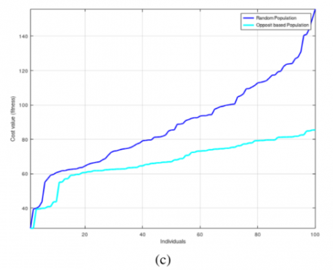
Figure 1 show the fitness of a population initialized randomly in comparison with an opposite based population using three different benchmark functions with 100 individuals in a space of [-5, +10], [-32.768, +32.768], [-5.12, +5.12] respectively, where the individuals of the opposite-based initialization are fitter than those of the random-based.
3.2 Saving the father
The BWO differs from other evolutionary algorithms with the step of cannibalism. The latter divides into three types where the famous one is the sexual cannibalism, in which the female consumes the male either before, during or after mating [13].
Generally, in spider’s society, the mother is fitter than the father. However, he can be fitter than his children so, destroying the male at the beginning of the procreation process leads to a loss of one of the best solutions which may influence the global results. To avoid this loss, we propose to remove the sexual cannibalism and delay destroying the father in the siblings cannibalism, which means at each generation if the father is fitter than his children, we save him for the next generation, otherwise we destroy him.
To get an idea of how many fit fathers are surviving each generation after sexual cannibalism, we have applied a test on the BWO algorithm with 100 individuals and the results are presented in Figure 2. We notice that in each generation at least 7% high-quality spiders survive, and in some cases, up to 35%.
Figure 1. Random population vs Opposite based population
Figure 2. Number of survived fit fathers
3.3 Adaptive procreation and mutation rates
BWOA distinguishes itself with parameters that are important for exploring the search space and avoiding the local optima trap. These parameters are procreation, mutation, and cannibalism rates. Procreation rate (Pc) is responsible for introducing new solutions into the population which means exploring the search space, mutation rate (Pm) helps the search process to escape from any local optima trap and keep the balance between exploration and exploitation, cannibalism rate (Cr) ensures high performance for the exploitation stage by transferring the search agents from local to the global stage and vice versa [13]. The values of these rates are determined statically prior to the execution of the algorithm, which critically affects its performance. To solve this problem and inspired by the work of Li and Sang [27], we propose an adaptive change of crossover and mutation probabilities, that ensures a high value of Pc at the beginning of the search and a low value in the last iterations, the same with mutation rate where its value is expected to rise as the number of generations increases. This process guarantees a balance between the exploration and exploitation. The adaptive description of the crossover and mutation probabilities is the following:
$P c=P c_{\max }-\left(P c_{\max }-P c_{\min }\right) \times e^{-\left(\frac{\text { MaxIter }}{\text { iter }} \quad\right)}$ (3)
$P m=P m_{\max }+\left(P m_{\max }-P m_{\min }\right) \times e^{-\left(\frac{\text { MaxIter }}{\text { iter }} \quad\right)}$ (4)
where, Pmmax, Pmmin are the upper and the lower bounds of mutation rate, the recommended parameters for these two mutation probabilities are 0.5 and 0.25 respectively. Pcmax, Pcmin are the upper and the lower bounds of crossover rate and the recommended parameters for these two crossover probabilities are 0.83 and 0.6. The parameter iter is the current iteration and MaxIter is the maximum number of iterations.
Algorithm 1: Modified Black Widow Algorithm
Input: MaxIter, Cannibalism rate, ub, lb, P mmax; P mmin; P cmax; P cmin;
Output: Near optimal solution to the objective function;
//Initialization
while (t<Maxiter) do
//Procreating and cannibalism;
Randomly select two solutions as parent from pop1;
Generate D children using Eq. (1) and Eq. (2).
Save the father if he is fitter than his children; Based on cannibalism rate destroy some of the children;
Save the remain solution into pop2;
end
//Mutation
Select a solution from pop1;
Randomly mutate one chromosome of the solution and generate a new solution;
ave the new one in pop3;
end
//Update
end
Figure 3. The flowchart of the proposed algorithm
Both of procreation rate and mutation rate change exponentially, which guarantees a constant Pc and Pm at the beginning of the search because of the high value of $\left(\frac{\text { MaxIter }}{\text { iter }}\right)$ in the first generations which means exploring the space first then, after performing the exploration the adaptation of the parameters starts where the Pc decreases and Pm increases hence the process of exploitation starts.
The flowchart of the Modified Black Widow Optimization MBWO is presented in Figure 3 and the pseudo-code is shown in Algorithm 1.
In order to investigate the effect of the modifications that we have made on the BWO algorithm, 19 optimization standard functions have been evaluated where the stop condition is the maximum number of iterations. The algorithm is compared with other bio-inspired approaches, which are BWO (Black Widow Optimization), ABWO (Adaptive Black Widow Optimization) [17], BBO (Bio-geography-based optimization) [28], GA (Genetic Algorithm) and IWO (invasive weed optimization) [29]. The algorithms have been implemented in an Octave environment using the same personal computer with windows 10 operating system (64-bit professional), and the following hardware settings: Core(TM) i7-8565U CPU @ 1.80GHz 1.99 GHz, 8 GB RAM, 1 TB hard drive.
4.1 Test functions
All the functions that have been used in this simulation are defined in Table 1, among these functions, f1, f2, f3, ..., f8 are uni-modal functions that have not many local optimum but only a global one, these functions are used to verify the convergence rate of the algorithm. The functions from f9 to f15 are multi-dimensional functions with many local optima, these functions are used to test the ability of the algorithm to jump from the local optima and avoid getting trapped in it. The remained functions f16, f17, f18, f19 are complexe two dimensional functions which are used to test the algorithm in handling problems with low dimensions.
4.2 Results on benchmark functions
The results presented in Table 3 are obtained after running each of the noticed algorithms 20 times with each function in the dimensions of 10, 20 and 30, and with 500 iterations where "Best" is the best result fitness returned by the algorithm in 20 runs, "Mean" and "Median" refer to the mean value and the median value of the cost returned in 20 runs respectively. "STD" is the value of the standard derivation of the algorithm, and it is a measure of how much dispersed the individuals are in relation to the mean. Therefor the lower the value of "STD", the more robust and reliable the algorithm is. All the values that are less than 10E-50 are supposed to be 0. The used parameters of each algorithm are set in Table 2.
From the results shown in Table 3, it is observed that our proposed algorithm MBWO provides better results than the mentioned experimental algorithms in most of benchmark functions.
Table 1. Test functions adopted for experiments
Table 2. Parameters values
|
Algorithm |
Parameters |
|
BWO |
Pc= 0:6; Pm=0:4; Cr=0:44 |
|
ABWO |
P cmin=0:6; Pcmax=0:8; Cr=0:5 |
|
P mmin = 0:2; P mmax = 0:4 |
|
|
MBWO |
P cmin = 0:6; Pcmax=0:83; P mmin = 0:25 |
|
P mmax = 0:5; Cr = 0:44 |
|
|
BBO |
keepRate = 0:6; Absorption Coeff = 0:9 |
|
P m = 0:4 |
|
|
GA |
P c = 0:67; P m = 0:33 |
|
IWO |
initial = 0:5; final = 0:001; Exponent = 2 |
|
seedmin = 0; seedmax = 5 |
In the case of functions with many local optima such as F9, F13 and F15, the MBWO outperformed the other algorithms in terms of “Best”, "Mean","Median" and "STD" values, proving its ability to escape from the local optima trap, since these functions are difficult to optimize, especially with F15 where the MBWO has placed results equal to the global optima in the dimensions of 20 and 30.
According to the results achieved for F3, F8 and F11, although the BWO and the adaptive BWO have returned the exact global optima in terms of "Best" in all dimensions and with F10 in the dimension of 20. However, in terms of “mean”,"median" and the standard derivation values the MBWO has provided results quite better than the others.
For the first function F1 (Sphere), MBWO outperformed the other algorithms in the dimension of 10. However, in the dimensions of 20 and 30 the performance of MBWO was a little bit weaker than BWO in the case of "Best", the same with F2 in the dimension of 30.
Considering the global optima of F16 and F18 functions are -1,-186.73 respectively, all the algorithms have achieved the exact global optima in terms of "Best" and "Median". However, in terms of "STD", the values returned by MBWO were the best ones. This proves that the algorithm achieves almost the same optimum in each independent run. With F17 (Schaffar 2), all the algorithms excluding IWO have achieved the global optima in terms of "Best". However, GA, ABWO and MBWO performed better with this function in the case of "Mean" and "Median".
With F7 (Dixon Price), the IWO was the best in returning the optimum results in all dimensions. The MBWO has returned the same optimum as that of the IWO in case of "Best". However, "Mean", "Median" and "STD" could not obtain acceptable results.
For the F12 function (Periodic), which has the optimum of 0.9, all the algorithms except the BBO have returned similar results in the dimensions of 20 and 30 in terms of "Best", and in the dimension of 10 only the MBWO achieved the best results.
The simulation results reveal that the MBWO has better solution performance on 10, 20, and 30-dimensional test functions as well as two-dimensional functions. It is mainly due to the introduction of opposite-based initialization, which ensures the high-quality of the initial population and increases the probability that the individuals will achieve the optimum solution faster, as is well observed from the values of the optimum returned by the algorithm. The addition of the adaptive adjustment of the parameters in Eq. (3) and Eq. (4) helps to protect the diversity of spiders in the search space and improves the optimization accuracy of the MBWO in each run, which is well observable from the values of the standard derivation. At the same time, saving the father each generation helps to accelerate the convergence speed in the later stages of iteration. The algorithm's performance and accuracy for solving complex high-dimensional functions are improved, as demonstrated by functions, and the problem of the algorithm's propensity to slip into a local optimum is resolved.
Table 3. Comparison of various algorithms
|
Function |
|
F1 |
|
|
F2 |
|
|
F3 |
|
|
|
Dim |
|
10 |
20 |
30 |
10 |
20 |
30 |
10 |
20 |
30 |
|
BWO |
Best |
2.19E-29 |
2.54E-37 |
1.88E-23 |
2.59E-24 |
4.84E-26 |
8.77E-24 |
0 |
0 |
0 |
|
|
Mean |
2.99E-07 |
2.12E-10 |
1.78E-08 |
3.36E-13 |
1.79E-14 |
8.45E-16 |
4.17E-06 |
2.07E-05 |
4.93E-31 |
|
|
Median |
1.43E-10 |
5.82E-18 |
3.02E-20 |
3.37E-15 |
1.84E-17 |
1.66E-16 |
8.66E-16 |
0 |
0 |
|
|
STD |
8.63E-07 |
4.92E-10 |
5.63E-08 |
9.57E-13 |
6.63E-14 |
1.92E-15 |
1.14E-05 |
5.01E-07 |
1.55E-30 |
|
ABWO |
Best |
1.34E-27 |
3.85E-30 |
3.54E-22 |
4.00E-20 |
2.55E-26 |
7.01E-23 |
0 |
0 |
0 |
|
|
Mean |
5.85E-08 |
8.16E-12 |
6.04E-10 |
3.72E-14 |
7.70E-15 |
1.41E-13 |
1.37E-07 |
2.21E-26 |
6.43E-05 |
|
|
Median |
1.45E-12 |
9.73E-21 |
2.37E-20 |
2.35E-14 |
5.42E-16 |
1.85E-16 |
0 |
0 |
0 |
|
|
STD |
2.32E-07 |
3.32E-11 |
1.91E-09 |
1.00E-13 |
1.98E-14 |
3.84E-13 |
5.16E-07 |
9.92E-26 |
2.03E-04 |
|
MBWO |
Best |
4.10E-64 |
2.03E-33 |
2.47E-22 |
5.10E-26 |
7.42E-27 |
9.06E-24 |
0 |
0 |
0 |
|
|
Mean |
6.88E-10 |
4.15E-17 |
3.83E-13 |
7.63E-15 |
1.22E-16 |
2.46E-17 |
7.77E-13 |
0 |
0 |
|
|
Median |
8.24E-13 |
9.69E-31 |
9.66E-21 |
1.03E-16 |
3.01E-19 |
7.30E-19 |
0 |
0 |
0 |
|
|
STD |
1.99E-09 |
1.86E-16 |
1.21E-12 |
1.61E-14 |
2.72E-16 |
6.60E-17 |
1.55E-11 |
0 |
0 |
|
GA |
Best |
1.00E-13 |
2.94E-07 |
5.32E-12 |
5.82E-24 |
1.91E-22 |
1.28E-20 |
9.11E-24 |
3.61E-18 |
2.81E-17 |
|
|
Mean |
9.49E-06 |
1.20E-03 |
8.35E-05 |
4.02E-10 |
3.36E-11 |
9.25E-14 |
1.98E-03 |
9.31E-05 |
7.18E-06 |
|
|
Median |
1.12E-07 |
1.11E-04 |
1.52E-03 |
9.80E-14 |
1.13E-16 |
3.44E-16 |
3.35E-05 |
1.85E-07 |
2.73E-07 |
|
|
STD |
3.45E-05 |
3.32E-03 |
3.81E-03 |
1.56E-09 |
1.03E-10 |
2.91E-13 |
8.00E-03 |
8.13E-03 |
2.06E-05 |
|
BBO |
Best |
1.06E-04 |
1.48E-02 |
9.60E-02 |
5.71E-14 |
3.09E-15 |
4.64E-15 |
4.22E-10 |
4.08E-10 |
1.80E-09 |
|
|
Mean |
2.60E-04 |
2.46E-02 |
1.08E-02 |
1.95E-13 |
1.40E-12 |
5.58E-13 |
2.82E-06 |
1.20E-06 |
8.09E-07 |
|
|
Median |
4.99E-04 |
2.48E-02 |
1.06E-01 |
1.95E-13 |
9.98E-14 |
6.17E-14 |
2.47E-07 |
1.70E-07 |
1.21E-07 |
|
|
STD |
1.06E-04 |
4.34E-03 |
1.08E-02 |
1.32E-13 |
3.97E-12 |
9.47E-13 |
8.75E-06 |
2.19E-06 |
1.32E-06 |
|
IWO |
Best |
1.40E-06 |
1.50E-05 |
5.85E-05 |
2.90E-10 |
8.25E-09 |
2.94E-08 |
3.61E-11 |
3.59E-10 |
4.84E-10 |
|
|
Mean |
2.62E-06 |
2.11E-05 |
8.35E-05 |
7.29E-09 |
3.42E-08 |
1.11E-07 |
6.50E-09 |
4.82E-08 |
6.80E-09 |
|
|
Median |
2.66E-06 |
2.25E-05 |
8.47E-05 |
4.58E-09 |
2.64E-08 |
1.12E-07 |
4.19E-09 |
4.49E-08 |
4.59E-09 |
|
|
STD |
6.33E-07 |
3.70E-06 |
1.45E-05 |
7.39E-09 |
2.70E-08 |
4.63E-08 |
6.75E-09 |
2.99E-08 |
6.02E-09 |
|
Function |
|
F4 |
|
|
F5 |
|
|
F6 |
|
|
|
Dim |
|
10 |
20 |
30 |
10 |
20 |
30 |
10 |
20 |
30 |
|
BWO |
Best |
3.75E-11 |
6.22E-03 |
1.31E-03 |
4.52E-12 |
2.93E-19 |
2.87E-13 |
9.46E-14 |
5.24E-05 |
7.98E-07 |
|
|
Mean |
4.35E-03 |
3.96E+00 |
1.33E+01 |
1.04E-03 |
9.30E-05 |
1.28E-05 |
4.75E-04 |
2.27E-02 |
2.85E-01 |
|
|
Median |
9.90E-05 |
1.42E+00 |
7.77E+00 |
2.17E-05 |
6.30E-04 |
3.57E-10 |
9.03E-08 |
4.07E-03 |
2.34E-01 |
|
|
STD |
8.95E-02 |
7.18E+00 |
1.78E+01 |
2.42E-03 |
2.01E-04 |
4.07E-05 |
2.10E-03 |
3.53E-02 |
2.74E-01 |
|
ABWO |
Best |
9.49E-11 |
4.28E-04 |
2.68E-04 |
1.91E-18 |
5.14E-19 |
2.02E-12 |
1.06E-15 |
1.36E-05 |
2.18E-05 |
|
|
Mean |
2.05E-02 |
2.24E+00 |
1.87E+02 |
2.06E-03 |
1.34E-04 |
8.11E-07 |
1.90E-04 |
3.69E-02 |
2.77E-01 |
|
|
Median |
1.05E-05 |
4.59E+01 |
1.07E+02 |
1.14E-05 |
7.54E-09 |
2.20E-11 |
5.34E-06 |
1.38E-02 |
1.29E-01 |
|
|
STD |
6.29E-02 |
4.68E+00 |
2.48E+02 |
5.11E-04 |
3.20E-04 |
2.56E-06 |
4.77E-04 |
5.15E-02 |
3.25E-01 |
|
MBWO |
Best |
3.01E-12 |
2.33E-05 |
2.43E-05 |
5.66E-22 |
7.63E-20 |
2.69E-13 |
1.23E-16 |
6.32E-09 |
1.13E-07 |
|
|
Mean |
1.60E-03 |
2.84E-01 |
2.43E+00 |
4.55E-04 |
2.38E-05 |
8.03E-09 |
5.37E-05 |
5.11E-03 |
8.37E-02 |
|
|
Median |
5.46E-06 |
1.18E-01 |
1.01E+00 |
2.05E-06 |
3.16E-11 |
1.00E-11 |
1.12E-07 |
1.58E-03 |
8.64E-03 |
|
|
STD |
5.49E-03 |
4.02E-01 |
2.72E+00 |
1.94E-04 |
8.85E-05 |
2.81E-08 |
2.20E-04 |
8.49E-03 |
1.39E-01 |
|
GA |
Best |
2.07E-04 |
3.69E-01 |
1.02E-01 |
7.38E-06 |
3.85E-05 |
8.18E-04 |
9.17E-09 |
6.28E-04 |
2.01E-02 |
|
|
Mean |
3.76E-02 |
4.13E+01 |
3.99E+01 |
1.07E-02 |
6.81E-02 |
1.20E-01 |
1.54E-02 |
8.07E-01 |
1.16E+00 |
|
|
Median |
3.66E-01 |
2.33E+01 |
1.08E+01 |
1.75E-03 |
1.26E-02 |
5.39E-02 |
4.29E-04 |
4.27E-01 |
5.78E-01 |
|
|
STD |
9.87E-01 |
5.43E+01 |
5.26E+01 |
4.19E-02 |
1.10E-01 |
1.63E-01 |
2.84E-02 |
1.25E-01 |
1.35E+00 |
|
BBO |
Best |
9.02E-02 |
1.65E+01 |
1.72E+02 |
3.71E-02 |
5.68E-01 |
2.14E+00 |
2.48E-03 |
6.13E-01 |
4.40E+00 |
|
|
Mean |
1.73E-01 |
3.35E+01 |
2.23E+02 |
5.26E-02 |
8.56E-01 |
2.36E+00 |
4.79E-03 |
8.28E-01 |
5.16E+00 |
|
|
Median |
1.71E-01 |
3.33E+01 |
2.27E+02 |
5.02E-02 |
8.77E-01 |
2.38E+00 |
4.77E-03 |
8.46E-01 |
4.93E+00 |
|
|
STD |
5.67E-02 |
7.28E+00 |
2.57E+01 |
9.94E-03 |
1.08E-01 |
1.55E-01 |
1.09E-03 |
1.82E-01 |
6.03E-01 |
|
IWO |
Best |
9.19E-06 |
1.00E+02 |
3.45E+03 |
3.15E-03 |
1.37E-02 |
3.58E-02 |
6.46E-06 |
1.44E-04 |
1.03E-03 |
|
|
Mean |
1.28E-05 |
2.16E+02 |
1.79E+04 |
4.26E-03 |
1.17E-02 |
4.76E-02 |
1.17E-04 |
6.23E-03 |
9.14E-02 |
|
|
Median |
1.35E-05 |
2.53E+02 |
1.47E+04 |
4.22E-03 |
1.70E-02 |
4.82E-02 |
1.22E-05 |
2.33E-03 |
9.59E-03 |
|
|
STD |
1.99E-06 |
8.08E+01 |
1.21E+04 |
5.74E-04 |
1.85E-03 |
6.98E-03 |
3.12E-03 |
2.33E-04 |
6.00E-01 |
|
Function |
|
F7 |
|
|
F8 |
|
|
F9 |
|
|
|
Dim |
|
10 |
20 |
30 |
10 |
20 |
30 |
10 |
20 |
30 |
|
BWO |
Best |
6.66E-01 |
6.70E-01 |
9.28E-01 |
0 |
0 |
0 |
2.1E+01 |
9.53E+01 |
4.91E+02 |
|
|
Mean |
7.20E-01 |
1.60E+00 |
4.23E+00 |
2.80E-15 |
1.40E-17 |
5.27E-22 |
2.73E+02 |
5.67E+02 |
1.396E+03 |
|
|
Median |
6.77E-01 |
1.02E+00 |
4.06E+00 |
1.39E-39 |
6.79E-33 |
7.44E-43 |
1.73E+02 |
5.00E+02 |
1.268E+03 |
|
|
STD |
9.33E-02 |
8.85E-01 |
1.63E+00 |
1.25E-14 |
6.00E-17 |
1.66E-21 |
2.87E+02 |
4.94E+02 |
8.26E+02 |
|
ABWO |
Best |
6.66E-01 |
6.84E-01 |
8.29E-01 |
0 |
0 |
0 |
2.40E+01 |
4.80E+01 |
4.53E+02 |
|
|
Mean |
7.21E-01 |
1.32E+00 |
3.66E+00 |
1.64E-21 |
1.80E-21 |
2.01E-28 |
2.56E+02 |
8.05E+02 |
1.54E+03 |
|
|
Median |
6.93E-01 |
1.06E+00 |
2.95E+00 |
5.08E-33 |
4.02E-42 |
5.40E-44 |
2.73E+02 |
5.53E+02 |
1.32E+03 |
|
|
STD |
6.30E-02 |
6.36E-01 |
1.09E+00 |
6.16E-21 |
8.05E-21 |
6.36E-28 |
1.60E+02 |
7.43E+02 |
4.32E+02 |
|
MBWO |
Best |
6.63E-01 |
6.70E-01 |
6.68E-01 |
0 |
0 |
0 |
1.13E+01 |
3.61E+01 |
3.60E+02 |
|
|
Mean |
6.80E-01 |
8.10E-01 |
1.46E+00 |
1.14E-27 |
7.23E-32 |
3.71E-36 |
1.22E+02 |
4.41E+02 |
8.58E+02 |
|
|
Median |
6.70E-01 |
7.79E-01 |
1.18E+00 |
1.34E-42 |
0 |
2.70E-48 |
9.53E+01 |
3.81E+02 |
8.10E+02 |
|
|
STD |
1.98E-03 |
3.18E-01 |
8.90E-01 |
5.11E-27 |
3.23E-30 |
1.08E-35 |
1.02E+02 |
3.06E+02 |
3.67E+02 |
|
GA |
Best |
6.66E-01 |
7.79E-01 |
4.13E+00 |
3.88E-39 |
0 |
1.25E-38 |
1.56E+01 |
5.25E+02 |
2.24E+03 |
|
|
Mean |
7.04E-01 |
9.97E+00 |
1.34E+01 |
7.09E-15 |
2.86E-08 |
3.56E-15 |
3.14E+02 |
1.56E+03 |
3.88E+03 |
|
|
Median |
6.73E-01 |
2.66E+00 |
1.38E+01 |
1.96E-25 |
2.28E-17 |
9.81E-19 |
2.21E+02 |
1.37E+03 |
3.83E+03 |
|
|
STD |
1.23E-01 |
5.09E+00 |
7.27E+00 |
2.29E-14 |
1.21E-07 |
8.40E-15 |
2.83E+02 |
7.34E+02 |
8.83E+02 |
|
BBO |
Best |
6.69E-01 |
1.33E+00 |
565E+00 |
4.58E-19 |
3.49E-09 |
4.67E-06 |
2.24E+01 |
3.89E+02 |
1.66E+03 |
|
|
Mean |
6.72E-01 |
1.83E+00 |
8.08E+00 |
1.10E-15 |
1.40E-08 |
1.12E-05 |
2.82E+02 |
1.02E+03 |
2.63E+03 |
|
|
Median |
6.71E-01 |
1.78E+00 |
8.19E+00 |
8.68E-16 |
2.66E-08 |
1.06E-05 |
2.35E+02 |
1.05E+03 |
2.60E+03 |
|
|
STD |
2.11E-03 |
3.43E-01 |
1.67E+00 |
1.06E-15 |
4.63E-08 |
7.64E-06 |
1.86E+02 |
3.75E+02 |
5.71E+02 |
|
IWO |
Best |
6.66E-01 |
6.67E-01 |
6.68E-01 |
7.61E-33 |
5.11E-28 |
2.84E-25 |
1.20E+03 |
2.59E+03 |
5.76E+03 |
|
|
Mean |
6.66E-01 |
6.67E-01 |
7.38E-01 |
3.32E-26 |
1.57E-27 |
3.17E-24 |
1.58E+03 |
3.65E+03 |
1.39E+03 |
|
|
Median |
6.66E-01 |
6.67E-01 |
6.71E-01 |
1.56E-26 |
1.13E-27 |
1.42E-24 |
1.56E+02 |
3.71E+03 |
6.73E+03 |
|
|
STD |
2.12E-06 |
1.77E-04 |
1.34E-01 |
5.35E-26 |
1.48E-27 |
3.58E-24 |
2.26E+02 |
4.95E+02 |
5.65E+02 |
|
Function |
|
F10 |
|
|
F11 |
|
|
F12 |
|
|
|
Dim |
|
10 |
20 |
30 |
10 |
20 |
30 |
10 |
20 |
30 |
|
BWO |
Best |
8.52E-14 |
0 |
5.68E-14 |
9.98E-02 |
9.98E-02 |
9.98E-02 |
9.00E-01 |
1.00E+00 |
1.00E+00 |
|
|
Mean |
2.03E-03 |
4.21E-03 |
8.76E-05 |
1.39E-01 |
1.29E-02 |
1.79E-01 |
9.85E-01 |
1.01E+00 |
1.03E+00 |
|
|
Median |
5.95E-05 |
3.44E-05 |
7.67E-09 |
1.09E-01 |
1.99E-01 |
1.99E-01 |
1.01E+00 |
1.00E+00 |
1.04E+00 |
|
|
STD |
1.28E-02 |
1.28E-02 |
1.84E-04 |
4.64E-02 |
4.70E-02 |
6.32E-02 |
3.68E-02 |
2.58E+03 |
7.86E-03 |
|
ABWO |
Best |
0 |
0 |
5.68E-14 |
9.99E-02 |
9.98E-02 |
9.98E-02 |
9.00E-01 |
1.00E+00 |
1.00E+00 |
|
|
Mean |
1.76E-02 |
2.41E-04 |
2.41E-05 |
9.99E-02 |
1.74E-01 |
1.69E-01 |
9.99E-01 |
1.00E+00 |
1.02E+00 |
|
|
Median |
4.60E-07 |
1.13E-08 |
8.52E-11 |
9.99E-02 |
1.99E-01 |
2.49E-01 |
1.01E-02 |
1.00E+00 |
1.00E+00 |
|
|
STD |
6.66E-01 |
1.02E-03 |
7.64E-05 |
7.90E-11 |
7.86E-02 |
8.23E-02 |
4.93E-02 |
3.23E-02 |
5.44E-03 |
|
MBWO |
Best |
0 |
0 |
5.68E-14 |
9.98E-02 |
9.98E-02 |
1.99E-01 |
9.00E-01 |
1.00E+00 |
1.00E+00 |
|
|
Mean |
1.26E-03 |
5.93E-05 |
3.36E-06 |
9.98E-02 |
1.24E-02 |
1.09E-01 |
9.70E-01 |
1.00E+00 |
1.00E+00 |
|
|
Median |
3.15E-08 |
2.84E-14 |
1.13E-13 |
9.98E-02 |
9.98E-02 |
1.99E-01 |
1.00E+00 |
1.00E+00 |
1.00E+00 |
|
|
STD |
1.03E-02 |
2.47E-04 |
1.06E-05 |
8.53E-12 |
4.44E-02 |
3.16E-02 |
3.68E-02 |
2.23E-04 |
2.60E-04 |
|
GA |
Best |
3.79E-08 |
8.47E-04 |
4.42E-04 |
9.98E-02 |
9.98E-02 |
1.99E-01 |
1.00E+00 |
1.00E+00 |
1.04E+00 |
|
|
Mean |
9.29E-02 |
6.70E-01 |
1.59E+00 |
1.19E-01 |
2.19E-01 |
3.49E-01 |
9.98E-01 |
1.01E+00 |
1.49E+00 |
|
|
Median |
9.35E-04 |
4.51E-02 |
1.52E+00 |
9.98E-02 |
1.99E-01 |
3.99E-01 |
1.00E+00 |
1.02E+00 |
1.29E+00 |
|
|
STD |
1.96E-01 |
1.74E+00 |
1.04E+00 |
5.23E-02 |
6.95E-02 |
7.07E-02 |
2.34E-02 |
3.05E-02 |
4.26E-01 |
|
BBO |
Best |
1.06E+00 |
1.13E+01 |
3.53E+01 |
9.98E-02 |
4.01E-02 |
8.37E-01 |
1.00E+00 |
1.05E+00 |
2.29E+00 |
|
|
Mean |
3.26E+00 |
1.48E+01 |
4.12E+01 |
1.04E-01 |
5.20E-01 |
9.41E-01 |
1.00E+00 |
1.09E+00 |
2.62E+00 |
|
|
Median |
3.05E+00 |
1.44E+01 |
4.14E+01 |
1.08E-01 |
5.15E-01 |
9.45E-01 |
1.00E+00 |
1.09E+00 |
2.68E+00 |
|
|
STD |
1.34E+00 |
2.14E+00 |
1.04E+00 |
4.64E-02 |
5.22E-02 |
5.72E-02 |
6.70E-04 |
2.23E-02 |
1.62E-01 |
|
IWO |
Best |
1.99E+00 |
1.19E+01 |
2.58E+01 |
6.09E+00 |
1.38E+01 |
2.08E+01 |
1.00E+00 |
1.00E+00 |
1.06E+00 |
|
|
Mean |
6.51E+00 |
2.80E+01 |
5.33E+01 |
8.58E+00 |
1.60E+01 |
2.24E+01 |
1.00E+00 |
1.00E+00 |
1.01E+00 |
|
|
Median |
6.96E+00 |
2.63E+01 |
5.47E+01 |
8.24E+00 |
1.60E+01 |
2.23E+01 |
1.00E+00 |
1.00E+00 |
1.01E+00 |
|
|
STD |
2.31E+00 |
9.90E+00 |
1.50E+01 |
1.12E+00 |
1.35E+00 |
1.06E+00 |
5.46E-07 |
3.23E-04 |
3.38E-04 |
|
Function |
|
F13 |
|
|
F14 |
|
|
F15 |
|
|
|
Dim |
|
10 |
20 |
30 |
10 |
20 |
30 |
10 |
20 |
30 |
|
BWO |
Best |
2.27E-10 |
7.54E-15 |
3.41E-10 |
7.38E-15 |
7.41E-11 |
5.72E-08 |
2.44E-10 |
8.88E-12 |
0 |
|
|
Mean |
1.64E-03 |
1.71E-04 |
6.47E-08 |
2.09E-08 |
1.94E-08 |
4.78E-07 |
1.32E-02 |
6.13E-02 |
1.71E-01 |
|
|
Median |
3.88E-05 |
2.05E-06 |
4.04E-10 |
1.14E-07 |
6.75E-09 |
2.23E-07 |
4.82E-02 |
2.91E-02 |
8.85E-02 |
|
|
STD |
5.83E-04 |
5.07E-04 |
1.88E-07 |
9.25E-08 |
2.40E-08 |
6.00E-07 |
1.13E-02 |
9.37E-02 |
2.00E-01 |
|
ABWO |
Best |
2.24E-14 |
7.54E-15 |
8.84E-10 |
8.38E-13 |
1.99E-11 |
4.99E-08 |
1.16E-08 |
0 |
1.12E-14 |
|
|
Mean |
4.17E-03 |
2.85E-04 |
4.02E-09 |
1.05E-09 |
8.97E-08 |
1.71E-06 |
2.10E-02 |
5.39E-02 |
2.41E-02 |
|
|
Median |
9.41E-05 |
2.17E-11 |
2.38E-09 |
2.53E-10 |
5.19E-08 |
2.06E-07 |
1.50E-02 |
2.08E-02 |
1.28E-01 |
|
|
STD |
1.19E-02 |
1.20E-03 |
9.02E-09 |
1.70E-09 |
2.05E-07 |
2.61E-06 |
1.61E-02 |
1.05E-01 |
3.04E-01 |
|
MBWO |
Best |
3.99E-15 |
7.54E-15 |
1.21E-10 |
6.67E-14 |
2.27E-12 |
2.87E-09 |
4.44E-16 |
0 |
0 |
|
|
Mean |
3.24E-05 |
7.19E-07 |
7.68E-10 |
1.45E-10 |
6.78E-09 |
2.13E-07 |
5.11E-03 |
4.00E-02 |
9.30E-03 |
|
|
Median |
3.84E-06 |
1.46E-14 |
4.22E-10 |
1.85E-11 |
1.76E-09 |
4.17E-08 |
4.30E-08 |
1.59E-02 |
9.58E-06 |
|
|
STD |
6.12E-05 |
3.10E-06 |
9.15E-10 |
2.56E-10 |
1.82E-08 |
5.01E-07 |
1.00E-03 |
1.37E-02 |
1.22E-01 |
|
GA |
Best |
9.78E-05 |
1.30E-04 |
1.96E-05 |
4.30E-07 |
1.66E-11 |
6.05E-09 |
1.99E-02 |
7.68E-08 |
2.93E-13 |
|
|
Mean |
3.91E-03 |
1.54E-01 |
9.60E-02 |
1.09E-09 |
3.56E-08 |
2.30E-06 |
8.63E-02 |
2.42E-01 |
2.57E-01 |
|
|
Median |
6.76E-03 |
3.22E-02 |
1.52E-02 |
2.40E-10 |
4.85E-09 |
7.37E-08 |
6.30E-02 |
1.21E-01 |
2.11E-02 |
|
|
STD |
9.33E-02 |
2.55E-01 |
1.96E-01 |
2.52E-09 |
6.40E-08 |
7.07E-06 |
1.49E-02 |
2.91E-01 |
4.56E-01 |
|
BBO |
Best |
9.22E-02 |
1.47E+00 |
2.44E+00 |
4.43E-10 |
8.09E-09 |
3.76E-08 |
1.71E-02 |
1.05E+00 |
1.29E+00 |
|
|
Mean |
1.65E-01 |
1.78E+00 |
2.78E+00 |
4.21E-08 |
2.01E-07 |
1.07E-06 |
2.71E-02 |
1.08E+00 |
1.35E+00 |
|
|
Median |
1.64E-01 |
1.80E+00 |
2.81E+00 |
8.99E-09 |
9.60E-08 |
1.41E-07 |
2.76E-02 |
1.08E+00 |
1.35E+00 |
|
|
STD |
4.36E-02 |
1.43E-01 |
1.70E-01 |
6.42E-08 |
2.77E-07 |
9.41E-07 |
4.93E-03 |
2.35E-02 |
5.13E+01 |
|
IWO |
Best |
1.70E-03 |
4.16E+00 |
1.81E+01 |
3.59E-07 |
2.68E-06 |
3.82E-06 |
2.50E+01 |
1.95E+02 |
3.18E+02 |
|
|
Mean |
9.19E-01 |
1.50E+01 |
1.86E+01 |
2.49E-06 |
7.61E-06 |
1.73E-03 |
7.06E+01 |
2.43E+02 |
4.38E+02 |
|
|
Median |
2.00E-03 |
1.81E+01 |
1.87E+01 |
2.03E-06 |
6.61E-06 |
1.92E-05 |
6.74E+01 |
2.50E+02 |
4.43E+02 |
|
|
STD |
4.10E+00 |
4.83E+00 |
3.22E+01 |
1.55E-06 |
4.21E-06 |
3.85E-03 |
2.10E+01 |
2.97E+01 |
6.32E+02 |
|
Function |
|
F16 |
|
F17 |
|
F18 |
|
|
F19 |
|
|
Dim |
|
2 |
|
2 |
|
2 |
|
|
2 |
|
|
BWO |
Best |
-1 |
|
0 |
|
-186.73 |
|
|
-2.0595 |
|
|
|
Mean |
-0.9958 |
|
3.86E-08 |
|
-182.61 |
|
|
-2.0244 |
|
|
|
Median |
-1 |
|
0 |
|
-186.73 |
|
|
-2.0417 |
|
|
|
STD |
1.45E-02 |
|
1.72E-07 |
|
1.43E+01 |
|
|
3.74E-02 |
|
|
ABWO |
Best |
-1 |
|
0 |
|
-186.73 |
|
|
-2.0626 |
|
|
|
Mean |
-0.9968 |
|
0 |
|
-186.73 |
|
|
-2.0626 |
|
|
|
Median |
-1 |
|
0 |
|
-186.73 |
|
|
-2.0626 |
|
|
|
STD |
1.42E-02 |
|
0 |
|
8.83E-02 |
|
|
6.61E-08 |
|
|
MBWO |
Best |
-1 |
|
0 |
|
-186.73 |
|
|
-2.0626 |
|
|
|
Mean |
-1 |
|
0 |
|
-186.73 |
|
|
-2.0626 |
|
|
|
Median |
-1 |
|
0 |
|
-186.73 |
|
|
-2.0626 |
|
|
|
STD |
4.48E-04 |
|
0 |
|
1.39E-10 |
|
|
4.68E-16 |
|
|
GA |
Best |
-1 |
|
0 |
|
-186.73 |
|
|
-2.0626 |
|
|
|
Mean |
-0.9995 |
|
0 |
|
-186.70 |
|
|
-2.0626 |
|
|
|
Median |
-1 |
|
0 |
|
-186.53 |
|
|
-2.0626 |
|
|
|
STD |
2.1655E-03 |
|
0 |
|
1.28E-01 |
|
|
4.68E-16 |
|
|
BBO |
Best |
-1 |
|
0 |
|
-186.73 |
|
|
-2.0626 |
|
|
|
Mean |
-1 |
|
2.88E-15 |
|
-186.73 |
|
|
-2.0626 |
|
|
|
Median |
-1 |
|
0 |
|
-186.73 |
|
|
-2.0626 |
|
|
|
STD |
3.72E-03 |
|
7.70E-15 |
|
4.33E-10 |
|
|
6.50E-15 |
|
|
IWO |
Best |
-1 |
|
3.01e-14 |
|
-186.73 |
|
|
-2.0626 |
|
|
|
Mean |
-1 |
|
3.14e-04 |
|
-186.73 |
|
|
-2.0626 |
|
|
|
Median |
-1 |
|
2.18e-13 |
|
-186.73 |
|
|
-2.0626 |
|
|
|
STD |
6.26E-04 |
|
9.66e-04 |
|
8.11e-07 |
|
|
3.48E-11 |
|
(a) F13 (dim=10)
(b) F13 (dim=10)-Zoom
Figure 4. Convergence of Ackley function
4.3 Convergence
The convergence speed of an algorithm is quite important to prove its efficiency and performance. With the aim of highlighting the fast convergence of the proposed approach, we have illustrated plots of the algorithms with different functions.
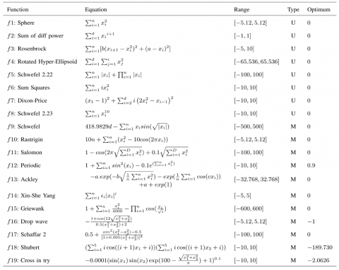
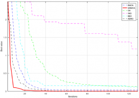
The convergence curves of the experiment methods are shown in Figure 4, Figure 5, Figure 6 and Figure 7, with the functions F13 (Ackley), F3 (RosenBrock), F15 (Griewank) and F19 (Cross in try) respectively, where the fast convergence of the MBWO within a smaller number of iterations is remarkable in comparison with the other algorithms.
All the figures are obtained after executing the algorithms for one independent run and 500 iterations with the mentioned functions in the dimensions of 10, 20, 30, and 2 respectively.
Furthermore, in Figure 6 with Griewank function, it is seen that the MBWO was the first in achieving the global optima. The same in Figure 7 with Cross in try function. These plots confirm that the MBWO can achieve the potential optimum faster due to the opposite-based intialization and can converge rapidly because of the decrease in the diversity that is well maintained by the adaptive adjustment of the parameters that are responsible for the exploration and exploitation of the search space.
(a) F3 (dim=20)
(b) F3 (dim=20)-Zoom
Figure 5. Convergence of RosenBrock function
(a) F15 (dim=30)
(b) F15 (dim=30)-Zoom
Figure 6. Convergence of Griewank function
(a) F19 (dim=2)
(b) F19 (dim=2)-Zoom
Figure 7. Convergence of Cross in Try function
This paper proposed a Modified Black Widow Optimization algorithm. The first modification was the use of the opposite-based initialization instead of the random one. The second was modifying the cannibalism process, where we suggested removing the sexual cannibalism and delaying destroying the father to the sibling cannibalism for the aim of avoiding the loss of fit solutions. Finally, an adaptive change of crossover and mutation probabilities is added for the purpose of keeping the balance between the exploration and exploitation. The validation is carried out after comparing the results of the MBWO algorithm with a set of bio-inspired approaches (BWO, ABWO, BBO, GA and IWO) using 19 benchmark functions in different dimensions. The MBWO has outperformed the algorithms in both achieving the best global optima and convergence speed. Despite all the results achieved by the proposed approach, this does not mean that it is the best algorithm developed, however it can be considered relevant and useful in solving various optimization problems.
The authors would like to thank the General Direction of Research and Development Technologies /Ministry of Higher Education and Scientific Research DGRSDT/MERS (ALGERIA) for its support.
[1] Manda, K., Satapathy, S.C., Poornasatyanarayana, B. (2012). Population based meta-heuristic techniques for solving optimization problems: A selective survey. International Journal of Emerging Technology and Advanced Engineering, 2(11): 206-211.
[2] Mori, N., Kita, H. (2000). Genetic algorithms for adaptation to dynamic environments-a survey. In 2000 26th Annual Conference of the IEEE Industrial Electronics Society. 2000 IEEE International Conference on Industrial Electronics, Control and Instrumentation. 21st Century Technologies, 4: 2947-2952. http://dx.doi.org/10.1109/IECON.2000.972466
[3] Mahmoodabadi, M.J., Nemati, A.R. (2016). A novel adaptive genetic algorithm for global optimization of mathematical test functions and real-world problems. Engineering Science and Technology, an International Journal, 19(4): 2002-2021. https://doi.org/10.1016/j.jestch.2016.10.012
[4] Bäck, T. (1992). Self-adaptation in genetic algorithms. In Proceedings of the First European Conference on Artificial Life, pp. 263-271.
[5] Davis, L. (1991). Handbook of Genetic Algorithms. New York: Van Nostrand Reinhold.
[6] Asselmeyer, T., Ebeling, W., Rosé, H. (1997). Evolutionary strategies of optimization. Physical Review E, 56(1): 1171. https://doi.org/10.1103/PhysRevE.56.1171
[7] Yao, X., Liu, Y., Lin, G. (1999). Evolutionary programming made faster. IEEE Transactions on Evolutionary Computation, 3(2): 82-102. http://dx.doi.org/10.1109/4235.771163
[8] Storn, R., Price, K. (1997). Differential evolution–A simple and efficient heuristic for global optimization over continuous spaces. Journal of Global Optimization, 11(4): 341-359. https://doi.org/10.1023/A:1008202821328
[9] Francone, F.D., Conrads, M., Banzhaf, W., Nordin, P. (1999). Homologous crossover in genetic programming. In GECCO, pp. 1021-1026.
[10] Fogel, D.B. (2000). What is evolutionary computation? IEEE Spectrum, 37(2): 26-32. https://doi.org/10.1109/6.819926
[11] Gomez, F.J. (2003). Robust non-linear control through neuroevolution. PhD thesis, The University of Texas at Austin. Technical Report AI-TR-03-303.
[12] Eiben, A.E., Rudolph, G. (1999). Theory of evolutionary algorithms: A bird's eye view. Theoretical Computer Science, 229(1-2): 3-9. https://doi.org/10.1016/S0304-3975(99)00089-4
[13] Hayyolalam, V., Kazem, A.A.P. (2020). Black widow optimization algorithm: A novel meta-heuristic approach for solving engineering optimization problems. Engineering Applications of Artificial Intelligence, 87: 103249. https://doi.org/10.1016/j.engappai.2019.103249
[14] Houssein, E.H., Helmy, B.E.D., Oliva, D., Elngar, A.A., Shaban, H. (2021). A novel black widow optimization algorithm for multilevel thresholding image segmentation. Expert Systems with Applications, 167: 114159. https://doi.org/10.1016/j.eswa.2020.114159
[15] Nanjappan, M., Natesan, G., Krishnadoss, P. (2021). An adaptive neuro-fuzzy inference system and black widow optimization approach for optimal resource utilization and task scheduling in a cloud environment. Wireless Personal Communications, 121(3): 1891-1916. https://doi.org/10.1007/s11277-021-08744-1
[16] Kumar, M. (2021). Energy efficient scheduling in cloud computing using black widow optimization. In Journal of Physics: Conference Series, 1950(1): 012063. http://dx.doi.org/10.1088/1742-6596/1950/1/012063
[17] Micev, M., Ćalasan, M., Petrović, D.S., Ali, Z.M., Quynh, N.V., Aleem, S.H.A. (2020). Field current waveform-based method for estimation of synchronous generator parameters using adaptive black widow optimization algorithm. IEEE Access, 8: 207537-207550. http://dx.doi.org/10.1109/ACCESS.2020.3037510
[18] Munirah, N.A., Remli, M.A., Ali, N.M., Nies, H.W., Mohamad, M.S., Wong, K.N.S.S. (2020). The development of parameter estimation method for Chinese Hamster Ovary model using black widow optimization algorithm. International Journal of Advanced Computer Science and Applications. http://dx.doi.org/10.14569/IJACSA.2020.0111126
[19] Ravikumar, S., Kavitha, D. (2021). IOT based autonomous car driver scheme based on ANFIS and black widow optimization. Journal of Ambient Intelligence and Humanized Computing, pp. 1-14. http://dx.doi.org/10.1007/s12652-020-02725-1
[20] Premkumar, K., Vishnupriya, M., Sudhakar Babu, T., et al. (2020). Black widow optimization-based optimal PI-controlled wind turbine emulator. Sustainability, 12(24): 10357. http://dx.doi.org/10.3390/su122410357
[21] Al-Rahlawee, A.T.H., Rahebi, J. (2021). Multilevel thresholding of images with improved Otsu thresholding by black widow optimization algorithm. Multimedia Tools and Applications, 80(18): 28217-28243. https://doi.org/10.1007/s11042-021-10860-w
[22] Sheriba, S.T., Rajesh, D.H. (2021). Energy-efficient clustering protocol for WSN based on improved black widow optimization and fuzzy logic. Telecommunication Systems, 77(1): 213-230. https://doi.org/10.1007/s11235-021-00751-8
[23] Panahi, F., Ehteram, M., Emami, M. (2021). Suspended sediment load prediction based on soft computing models and Black Widow Optimization Algorithm using an enhanced gamma test. Environmental Science and Pollution Research, 28(35): 48253-48273. http://dx.doi.org/10.1007/s11356-021-14065-4
[24] Mukilan, P., Semunigus, W. (2021). Human object detection: An enhanced black widow optimization algorithm with deep convolution neural network. Neural Computing and Applications, 33(22): 15831-15842. https://doi.org/10.1007/s00521-021-06203-3
[25] Tizhoosh, H.R. (2005). Opposition-based learning: A new scheme for machine intelligence. In International Conference on Computational Intelligence for Modelling, Control and Automation and International Conference on Intelligent Agents, Web Technologies and Internet Commerce (CIMCA-IAWTIC'06), 1: 695-701. http://dx.doi.org/10.1109/CIMCA.2005.1631345
[26] Rahnamayan, S., Tizhoosh, H.R., Salama, M.M. (2007). A novel population initialization method for accelerating evolutionary algorithms. Computers & Mathematics with Applications, 53(10): 1605-1614. https://doi.org/10.1016/j.camwa.2006.07.013
[27] Li, Y.B., Sang, H.B., Xiong, X., Li, Y.R. (2021). An improved adaptive genetic algorithm for two-dimensional rectangular packing problem. Applied Sciences, 11(1): 413. https://doi.org/10.3390/app11010413
[28] Simon, D. (2008). Biogeography-based optimization. IEEE Transactions on Evolutionary Computation, 12(6): 702-713. https://doi.org/10.1109/TEVC.2008.919004
[29] Xing, B., Gao, W.J. (2014). Invasive weed optimization algorithm. In Innovative Computational Intelligence: A Rough Guide to 134 Clever Algorithms, pp. 177-181. https://doi.org/10.1007/978-3-319-03404-1_13