Wiharto* | Fikri Hashfi Nashrullah | Esti Suryani | Umi Salamah | Nurcahya Pradana Taufik Prakisya | Sigit Setyawan
© 2021 IIETA. This article is published by IIETA and is licensed under the CC BY 4.0 license (http://creativecommons.org/licenses/by/4.0/).
OPEN ACCESS
The disease in tomato plants, especially on tomato leaves will have an impact on the quality and quantity of tomatoes produced. Handling disease on tomato leaves that must be done is to detect the type of disease as early as possible, then determine the treatment that must be done. Detection of its types of tomato plant diseases requires sufficient knowledge and experience. The problem is that many beginner farmers in growing tomatoes do not have much knowledge, so they have failed in growing tomatoes. Based on these cases, this study proposes a model for the early detection of disease in tomato leaves based on image processing. The research method used is divided into 5 stages, namely preprocessing, segmentation, feature extraction, classification, and performance evaluation. The feature extraction stage used is texture-based with Gabor filters and color-based filters. The final decision is determined by the Support Vector Machine (SVM) classification algorithm with the Radial Basis Function (RBF) kernel. The test results of the tomato leaf disease detection system produced an average performance parameter of 98.83% specificity, 90.37% sensitivity, 90.34% F1-score, 90.37% accuracy, and 94.60% area under the curve (AUC). Referring to the resulting of the AUC performance, the tomato leaf disease detection system is in the very good category.
Gabor filter, machine learning, support vector machine, texture, color, tomato disease
Tomato (Solanum Lycopersicum) is one of the main ingredients in making food in Indonesia. This plant can be made as food, beverage, vegetable, medicine, and even industrial raw materials. The wide use of tomatoes makes market demand very high. Currently, tomatoes are the 5th popular horticultural commodity in Indonesia, behind chilies, shallots, potatoes, and cabbage with a total production in 2018 of 0.98 million tons.
Planting tomato plants has many obstacles, some of which are due to pests or diseases of the tomato plant itself. Diseases in plants and the lack of expertise of farmers in Indonesia in distinguishing diseased leaf characteristics and types are problems that result in delays in handling which have an impact on decreasing productivity. Not only a problem in Indonesia, but plant diseases are also a problem in the majority of other developing countries. Several plant diseases are often caused by several pathogens including bacteria [1], viruses [2], and also fungi. The following are pathogens that commonly attack tomato plants, including tomato bacterial spot, early blight, late blight, leaf mold, septoria leaf spot, two-spotted spider mites, target spot, tomato mosaic virus, tomato yellow leaf curl virus, and bacterial spot [3].
The cause of disease in the tomato plant itself is quite difficult to detect because there are several similarities in features and shapes. In addition to the similarity in characteristics, some farmers do not recognize the terms of pathogens that attack tomato plants and only look directly manually and predict the presence of disease or not. The existence of ignorance of pathogens or diseases that attack tomato plants can interfere with tomato productivity and decrease.
The development of machine learning has led to a lot of research which done to solve these problems. Research conducted by Sethy et al. [3], tried to develop a plant disease detection model using automatic plant leaf images. Detection is performed using texture-based feature extraction methods with Gray Level Co-occurrences Matrix (GLCM), shape-based (minimum enclosing rectangle), color-based, and combinations thereof. Subsequent research conducted by Mollazade et al. [4] also used textures to detect disease in horticultural crops. Feature extraction is performed using statistical methods of image histogram, GLCM, and Gray level run length matrix. The classification process uses an adaptive neuro-fuzzy inference system (ANFIS). The use of texture and color-based feature extraction was also used in the research of Madiwalar et al. [5]. This study used the GLCM feature extraction method, based on color, and Gabor filters. The final result is determined using the Support Vector Machine (SVM) classification algorithm. The use of Gabor filters is very effective for detecting disease spots on plant leaves and has better performance when compared to GLCM.
The use of the SVM algorithm for disease detection in tomato plant leaves has also been widely used in a number of studies. Padol and Yadav [6] research used feature extraction based on shape, color and texture, preceded by a segmentation process using k-means clustering. Research by Hlaing and Zaw [7] used feature extraction based on statistical texture and color. Furthermore, Genitha et al. [8] research used principal component analysis (PCA) for the feature extraction process, to be further classified by SVM with a linear kernel. The SVM algorithm has a number of kernels that can be used, research by Mokhtar et al. [9] conducted tests for a number of kernels, namely Cauchy, Invmult, and Laplacian. This study using feature extraction with the Gabor wavelet transform method. Besides, research that emphasizes the use of SVM kernels was also carried out by Jayanthi and Shashikumar [10], namely using multi-kernel SVM to detect dau disease in tomato plants.
Feature extraction used in a number of studies that have been carried out varies widely. Feature extraction using Gabor filters has the advantage of feature extraction digital images by analyzing the texture of the object in the image, the sides of the object, and its frequency [11-13]. The function of feature extraction with Gabor filters is also shown in the research of Gadade and Kirange [14]. This study shows that the feature extraction Gabor filter is better than GLCM and Speeded up robust feature (SURF), and this study also shows that the SVM capability is better than the decision tree, kNN, and naïve bayesian algorithms. The ability of Gabor filters is also shown in a study conducted by Bhagavathy et al. [15]. This study proposes a Gabor filter texture descriptor with a rayleigh approach and makes a comparison with a Gabor filter texture descriptor using a gaussian approach. This study proves that the modified texture descriptors are comparable in performance, but with almost half the dimensions and less computational costs. The use of Gabor filters is also not only limited to the leaves of the tomato plant but the leaves of the vine, with the good ability [16].
Referring to a number of studies that have been carried out related to disease detection in tomato leaves, it can be seen in general the stages taken. These stages include preprocessing, segmentation, feature extraction, classification, and performance evaluation. At each stage, there are also a number of methods that can be used, as explained in the research of Singh et al. [17]. Feature extraction with a Gabor filter was able to extract the diseased features of tomato leaves well. Furthermore, for classification, the support vector machine is able to provide better performance than a number of previous studies, which was also confirmed in the research of Sunny and Gandhi [18]. Based on this, this study developed a leaf disease detection model in tomato plants using the otsu thresholding segmentation. Feature extraction uses Gabor filters and color based, with a classification algorithm using a support vector machine (SVM) [19]. The performance is measured by referring to the confusion matrics table. The performance parameters used are sensitivity, specificity, an area under the curve (AUC), F1-Score, and accuracy.
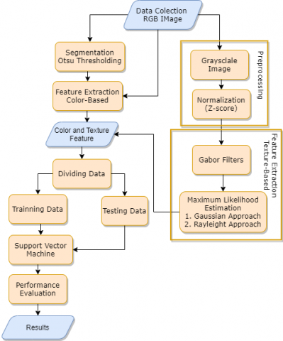
The research method in developing a model for disease detection in tomato leaves is divided into several stages. The first stage is preprocessing, segmentation, feature extraction, classification, and performance evaluation. The research methods used are shown in Figure 1.
2.1 Preprocessing
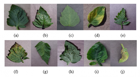
At this stage, prepare the dataset used in research for the learning and testing process. Tomato leaf image data is divided into two main groups, namely images of healthy tomato leaves and images of diseased tomato leaves. The image of diseased tomato leaves is further divided into 10 types of diseases, as shown in Table 1. The tomato leaf image data can be obtained from the public dataset at the link: https://github.com/spMohanty/PlantVillage-Dataset. The tomato leaf image is an RGB (red, green, blue) image with a size of 256 x 256 pixels. The RGB image is then converted into grayscale, then normalization is carried out using the z-score [20]. The data distribution for each type of disease can be seen in Table 1, while an example of an image of a leaf affected by disease is shown in Figure 2.
Figure 1. Research methods
Table 1. Distribution of the tomato leaf dataset
|
No |
Dataset Name |
Amount |
|
1 |
Tomato bacterial spot |
2127 |
|
2 |
Tomato Early Blight |
2400 |
|
3 |
Tomato Healthy |
2407 |
|
4 |
Tomato Late Blight |
2314 |
|
5 |
Tomato Leaf Mold |
2352 |
|
6 |
Tomato Septoria Leaf Spot |
2181 |
|
7 |
Tomato Spider Mites Two Spotted Spider Mite |
2180 |
|
8 |
Tomato Target Spot |
2284 |
|
9 |
Tomato Mosaic Virus |
2238 |
|
10 |
Tomato Yellow Curl Virus |
2451 |
2.2 Segmentation
The second stage in this research is the segmentation of tomato leaf images. Segmentation was carried out using the Otsu thresholding method [21]. The first step in this segmentation process is to make a histogram. Then, the histogram will determine the number of pixels for the gray level. After creating the histogram, the next step is to find the value of the number of classes, the class average, and the class variants. Pixels will be classified into two classes (for example divided into 2 classes), namely K0 and K1, background for class K0, and foreground for class K1 with a threshold at levels k to L which is the number of gray values (256 for 8 -bit images).
K0 is represented in pixels with a level of gray [1,2,3,…,, K] and K1 is represented in pixels with a level of [k+1,…,L]. The next step is to determine the inter-class variants. This inter-class variant aims to find the threshold value of a grayscale image. This threshold value will be used as a reference for converting a grayscale image to a binary image. Each image has a different threshold value [22]. In this study, the segmentation is divided into 3 classes/regions.
Figure 2. Image sample from each dataset. (a) Bacterial spot, (b) Early blight, (c) Healthy, (d) Leaf mold, (e) Mosaic virus, (f) Septoria leaf spot, (g) Spider mites, (h) Target spot, (i) Yellow leaf curl, (j) Late blight
2.3 Feature extraction color-based
The next stage is feature extraction. Feature extraction was carried out on a color basis. Color feature extraction is based on the presence of a color dataset (RGB) and also the characteristics of the dataset which tend to have a level of color similarity to the background, leaf objects, and disease objects. The color features taken are the mean and standard deviation of the RGB color features as well as the mean and standard deviation of the segmentation results using the multi-Otsu threshold with the color feature parameter a * color model CIE L* a* b*. The use of the algorithm and color model is based on previous research who mentioned the effectiveness of the algorithm [23]. The RGB value is obtained from the original image, while the L* a* b* color model is obtained by converting RGB to CIE XYZ then into CIE L* a* b* using Eqns. (1) and (2).
[XYZ]=[0.4124530.3575800.1804230.2126710.7151600.0721690.0193340.1191930.950227]∗[RGB] (1)
The conversion of XYZ to Lab can be seen in Eq. (2):
L∗=116(YYn)1/3−16, for YYn>0.008856
L∗=903.3YYn, others
a∗=500∗(f(X/Xn)−f(Y/Yn))
b∗=200∗(f(Y/Yn)−f(Z/Zn)) (2)
where, Xn,Yn,Zn is a reference value set by CIE.
2.4 Feature extraction texture-based
The next step is texture-based feature extraction using a Gabor filter. Before carrying out the texture-based feature extraction process, first, the color conversion process is carried out from the RGB color model to grayscale. The feature extraction method used is the Gabor Filter. Gabor filter itself is a sinusoidal function modulated by the Gaussian function [12]. The Gabor filter method is often used to detect edges, lines, and shapes [24]. The output produced by the 2D Gabor filter is a real and imaginary part that can be represented by a feature magnitude. The Gabor kernel can be generated using Eq. (3).
g(x,y,θ,σ,f)=12πσ2exp{−x2+y22σ2}×exp{2πif(xcosθ+ysinθ)} (3)
In Eq. (3), (x, y) are the coordinates of the Gabor filter, σ is the standard deviation of the envelope Gaussian, i=√−1 is the imaginary number, f is the frequency which is the inverse of wavelength λ,θ is the orientation and b (bandwidth) is the bandwidth used to calculate the standard deviation with the frequency relationship [24]. The use of the right parameters is an important thing in looking for texture characteristics. In this Gabor filter process, researchers used input parameters, namely 8 orientations and 5 frequencies [12]. The input parameters for the Gabor filter are as in Eqns. (4)-(6).
σ=1π√ln22⋅2b+12b+1fb(bandwidth)=1 (4)
θ=(0,π6,π4,π3,π2,π2+π6,π2+π4,π2+π3)=(0∘,,30∘,45∘,60∘,90∘,120∘,135∘,150∘) (5)
fk=(fmax (6)
After obtaining the Gabor kernel, an image input convolution is carried out using the kernel. After obtaining the results of the convolution, then the feature magnitude will also be obtained using Eqns. (7) and (8).
\mathrm{g} \mathrm{O}_{\mathrm{u}, \mathrm{v}}(\overrightarrow{\mathrm{z}})=\mathrm{I}(\overrightarrow{\mathrm{z}}) * \psi_{\mathrm{u}, \mathrm{v}}(\overrightarrow{\mathrm{z}}) (7)
\mathrm{M}_{\mathrm{u}, \mathrm{v}}(\overrightarrow{\mathrm{z}})=\sqrt{\operatorname{Re}^{2}\left\{\mathrm{O}_{\mathrm{u}, \mathrm{v}}(\overrightarrow{\mathrm{z}})\right\}+\operatorname{Im}^{2}\left\{\mathrm{O}_{\mathrm{u}, \mathrm{v}}(\overrightarrow{\mathrm{z}})\right\}} (8)
An estimation of the feature magnitude parameter is carried out using the maximum likelihood estimation with a Gaussian approach to obtain an estimation of the parameter magnitude value. Parameter estimation can be done using Eqns. (9)-(15).
Magnitude:
X=\left\{x_{1}, x_{2}, \ldots, x_{n}\right\} (9)
Gaussian probability density function:
\mathrm{p}(\mathrm{x} \mid \mu, \sigma)=\frac{1}{\sqrt{2 \pi} \sigma} \exp \left\{-\frac{(\mathrm{x}-\mu)^{2}}{2 \sigma^{2}}\right\} (10)
The likelihood function of Gaussian distribution:
\begin{array}{rl}\mathrm{L}(\mu, \sigma \mid \mathrm{x})=\prod_{\mathrm{i}=1}^{\mathrm{N}} & \mathrm{p}\left(\mathrm{x}_{\mathrm{i}} \mid \mu, \sigma\right) =\frac{(2 \pi)^{-\frac{\mathrm{N}}{2}}}{\sigma^{\mathrm{N}}} \exp \left\{-\frac{\sum_{\mathrm{i}=1}^{\mathrm{N}}(\mathrm{x}-\mu)^{2}}{2 \sigma^{2}}\right\}\end{array} (11)
The log-Likelihood function of Gaussian distribution:
\mathrm{L}(\mu, \sigma \mid \mathrm{x})=-\frac{1}{2} \mathrm{~N} \log 2 \pi-\mathrm{N} \log \sigma-\frac{\sum_{\mathrm{i}=1}^{\mathrm{N}}(\mathrm{x}-\mu)^{2}}{2 \sigma^{2}} (12)
First Estimator:
\hat{\mu}=\frac{\sum_{\mathrm{i}=1}^{\mathrm{N}} \mathrm{X}_{\mathrm{i}}}{\mathrm{N}} (13)
Second Estimator:
\widehat{\sigma}=\sqrt{\frac{\sum_{\mathrm{i}=1}^{\mathrm{N}}\left(\mathrm{x}_{\mathrm{i}}-\hat{\mathrm{u}}\right)^{2}}{\mathrm{~N}}} (14)
So, for the gaussian feature approach, it can be formed like Eq. (15):
\mathrm{f}_{\mathrm{u} \sigma}=\left\{\hat{\mu}_{1}, \widehat{\sigma}_{1}, \ldots, \hat{\mu}_{\mathrm{n}}, \widehat{\sigma}_{\mathrm{n}}\right\} (15)
In addition to using the gaussian approach, this study also makes comparisons using the Rayleigh approach as in research [15]. The estimation of parameters with the Rayleigh assumption can be done using Eqns. (16)-(21).
Rayleigh probability density function:
p(x \mid \gamma)=\frac{x}{\gamma^{2}} \exp \left\{-\frac{x^{2}}{2 \gamma^{2}}\right\} (16)
The likelihood function of X under Rayleigh assumption:
\mathrm{L}(\gamma \mid \mathrm{x})=\left(\frac{1}{\gamma^{2}}\right)^{\mathrm{N}} \prod_{\mathrm{i}=1}^{\mathrm{N}} \mathrm{x}_{\mathrm{i}} \exp \left\{-\frac{\mathrm{x}^{2}}{2 \gamma^{2}} \sum_{\mathrm{i}=1}^{\mathrm{N}} \mathrm{x}_{\mathrm{i}}^{2}\right\} (17)
The log-Likelihood function of X under Rayleigh assumption:
\mathrm{L}(\gamma \mid \mathrm{x})=\mathrm{N}\{\log 1-\log \gamma\}+\sum_{\mathrm{i}=1}^{\mathrm{N}} \log \mathrm{x}_{\mathrm{i}}-\frac{1}{2 \gamma^{2}} \sum_{\mathrm{i}=1}^{\mathrm{N}} \mathrm{x}_{\mathrm{i}}^{2} (18)
Estimator:
\gamma=\sqrt{\frac{1}{2 N} \sum_{i=1}^{N} x_{i}^{2}} (19)
So, the Rayleigh feature approach can be formed like an Eq. (20).
\mathrm{f}_{\gamma}=\left\{\hat{\gamma}_{0,0}, \hat{\gamma}_{0,1}, \ldots, \hat{\gamma}_{\mathrm{u}-1, \mathrm{v}-1}\right\} (20)
The Rayleigh estimator can also be calculated directly using the Gaussian estimator if it has been obtained previously using Eq. (21).
\hat{\gamma}=\sqrt{\frac{1}{2}\left\{\hat{\mu}^{2}+\widehat{\sigma}^{2}\right\}} (21)
2.5 Classification
The next stage is the classification process. The data classification process is divided into two, namely training and testing with a composition of 70% for training and 30% for testing. Classification is done using the multiclass Support Vector Machine (SVM) algorithm. The kernel method used in SVM is the Radial Basis Function. The RBF kernel can be written as Eq. (22).
\mathrm{K}(\mathrm{a}, \mathrm{b})=\mathrm{e}^{-\gamma(\mathrm{a}-\mathrm{b})^{2}} (22)
The square of the Euclidean distance between two data points 'a' and 'b' can be written as (a-b)^{2}. In addition, there are 2 parameters used in the RBF kernel, namely C and gamma. The parameter C or cost is a penalty for misclassifying a data point where when C is small, the classifier forgives the data points that are misclassified (high bias, low variance). However, when C is large, the classifier will not tolerate data misclassification. Meanwhile, gamma is a parameter that determines the decision area. When gamma is low, the decision boundary 'curve' is very low and thus the decision area is very wide [19].
2.6 Performance evaluation
The final step after obtaining labeling for each image based on color and texture-based features is to evaluate the system performance. Performance evaluation is done by calculating the parameters of sensitivity, specificity, area under the curve, F1-score, and accuracy. The calculation of performance parameters refers to the confusion matrix table for 10 classes and is then simplified into 2 classes, as shown in Table 2. Based on Table 2, calculations are carried out using Eqns. (23)-(27).
Table 2. Confusion matrix
|
Actual Class |
Predictive Class |
|
|
Positive |
Negative |
|
|
Positive |
TP |
FN |
|
Negative |
FP |
TN |
Sensitivity =\mathrm{SEN}=\frac{\mathrm{TP}}{\mathrm{TP}+\mathrm{FN}} (23)
Specificity =\mathrm{SPE}=\frac{\mathrm{TN}}{\mathrm{TN}+\mathrm{FP}} (24)
\mathrm{AUC}=\frac{\mathrm{SEN}+\mathrm{SPE}}{2}[25] (25)
Accuracy =A C C=\frac{T P+T N}{T P+F N+F P+T N} (26)
\mathrm{F} 1-\mathrm{Score}=\frac{2 \mathrm{TP}}{2 \mathrm{TP}+\mathrm{FN}+\mathrm{FP}} (27)
This section discusses the results of testing a model for a disease detection system in tomato leaves. Results will be presented for each stage.
3.1 Testing environment
This research was tested using the Python programming language assisted by the web-based editor Jupyter notebook software. The hardware specifications used for the experiment were a laptop with an Intel © Core © i5-6200U CPU @ 2.30 GHz, 8 GB RAM, and an Nvidia Geforce 930mx GPU.
3.2 The result feature extraction based-color
The selection of color features is based on the presence of a colored dataset and also the characteristics of the dataset which tend to have a similarity level to the background, leaf objects, and disease objects. One of the color features extracted or obtained from the dataset is the RGB color feature. This RGB color feature is characterized by the mean and standard deviation. The following is a feature of a leaf image with the viral mosaic disease.
(R, G, B)=\left[\begin{array}{ccc}{[179,171,174]} & \cdots & {[133,124,145]} \\ \vdots & \ddots & \vdots \\ {[104,89,108]} & \cdots & {[93,78,97]}\end{array}\right]
\mu(R)=116.244140625, \sigma(R)=40.9338809211793
\mu(G)=113.269454956, \sigma(G)=35.045435312442216
\mu(B)=121.752685547, \sigma(B)=46.84515285554443
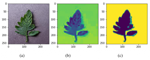
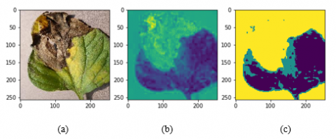
In addition to the RGB feature, another feature that is extracted is the color feature from the segmentation results to get only healthy leaves. Segmentation begins by taking the color a* in the L* a* b* color model converted from the RGB color model which is a green to the red color range. The color selection a* in L* a* b* is based on the color of the leaves which tend to be green and the color of the disease is brownish. After getting a* on the L*a*b* color model, then the thresholding is done. The test results for the types of viral mosaic disease and late blight are shown in Figure 3 and Figure 4.
Figure 3. Image mosaic virus: (a) Original image of the viral mosaic. (b) a* color image of L*a*b*. (c) Image threshold results
Figure 4. Image of late blight disease: (a) Original image of late blight. (b) a* color image of L*a*b*. (c) Image threshold results
Figure 5. The result of the Gabor filter
Figure 6. Image magnitude resulting from convolution (Virus mosaic)
Figure 7. Image magnitude resulting from convolution (Late-blight)
3.3 The result of feature extraction texture-based
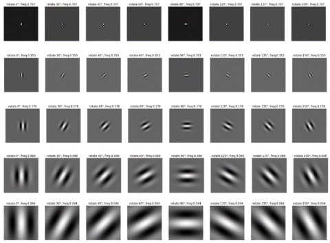
The aim of the feature texture extraction is to determine the texture of the leaves starting from the object's roughness, the sides of the object, horizontal lines, and vertical lines. Feature extraction is carried out using a Gabor filter. The Gabor filter is generated by Eqns. (3)-(6). Each parameter produces a different filter according to the frequency level and orientation. This is done because basically, every object has different characteristics that cannot be determined by one frequency and one orientation. A Gabor filter with 8 orientations and 5 frequencies resulting is shown in Figure 5.
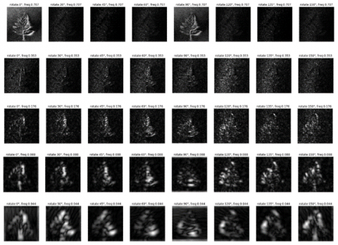
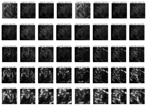
The next process, after obtaining 40 pieces of Gabor filters, then performed texture feature extraction. Feature extraction is carried out by convolution between the tomato leaf image that has been converted to grayscale and has been normalized with this Gabor filter. The results of feature extraction with the Gabor filter, for examples of types of leaf disease, the mosaic virus can be shown in Figure 6, while for the late blight is shown in Figure 7.
In the next stage after obtaining the magnitude of all diseased plant labels as well as healthy plants, the magnitude will be carried out again by feature extraction based on the maximum likelihood estimation (MLE) using the Gaussian approach and also the Rayleigh approach. This is done because the result of the feature magnitude is too complex to be used as a feature. The result of feature extraction is in the form of mean and standard deviation both from the results of the Gaussian and Rayleigh approaches.
3.4 Classification results
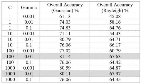
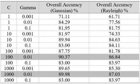
The results of the color-based and texture-based feature extraction process using a Gabor filter, in the form of mean and standard deviation, are the features of tomato leaves. Based on these results, the next step is classification using the Support Vector Machine algorithm. The kernel that is used to improve SVM performance is the RBF kernel. Referring to Eq. (22), the parameters used in the RBF kernel for SVM are gamma = 0.01 and C = 100. These parameters are obtained by experiments that have been carried out by trying several parameters, as shown in Table 3 and Table 4. The test results are shown in Table 3 using texture-based feature extraction using a Gabor filter with a gaussian and Rayleigh approach, while Table 4 shows the performance when combined with color-based feature extraction. In the Table 4 shows that the addition of color-based feature extraction is able to provide performance improvements. Best performance when using Gabor filters with a gaussian approach.
Table 3. Testing the RBF kernel variable (Texture)
Table 4. Testing the RBF kernel variable (Texture+Color)
Table 5. Performance measurement results for each type of disease
|
Class Label |
SPE |
SEN |
AUC |
F1-Score |
ACC |
|
Bacterial spot |
98.76 |
96.98 |
97.87 |
93.64 |
98.56 |
|
Early blight |
98.27 |
81.90 |
90.09 |
83.43 |
96.52 |
|
Healthy |
99.39 |
98.57 |
98.98 |
96.88 |
99.30 |
|
Late blight |
97.78 |
85.08 |
91.43 |
83.55 |
96.43 |
|
Leaf mold |
99.03 |
92.06 |
95.55 |
92.06 |
98.27 |
|
Mosaic virus |
99.28 |
93.81 |
96.55 |
93.96 |
98.68 |
|
Septoria leaf spot |
98.73 |
87.78 |
93.26 |
88.55 |
97.55 |
|
Spider mites |
98.77 |
87.78 |
93.28 |
88.69 |
97.58 |
|
Target spot |
98.87 |
86.03 |
92.45 |
88.06 |
97.48 |
|
Yellow leaf curl |
99.45 |
93.65 |
96.55 |
94.55 |
98.82 |
The calculation of the performance of the detection system is carried out by referring to Table 2, with the calculation of each performance parameter using Eqns. (23)-(27). The classification results for each type of disease using SVM and with kernel parameters RBF gamma = 0.01 and C = 100 can be shown in Table 5. The texture-based feature extraction method used is a Gabor filter with a gaussian approach and color-based feature extraction.
3.5 Discussion
The test results shown in Table 5 show that with reference to the parameters specificity, sensitivity, area under the curve, F1-score and accuracy. Referring to the sensitivity performance parameter, it shows that the early blight class has the lowest percentage followed by the late blight class, target spot, and Septoria leaf spot. The low ability of the detection model for this type of disease is due to the ability of the feature extraction method, Gabor filter, and feature extraction color-based, resulting in features from these four classes that have similar features with other classes. The early blight class has similar features to late blight and Septoria leaf spot. The target spot class has similar features to spider mites and viral mosaics. This is reinforced by the misclassification of these classes in the confusion matrix.
The test results show that the use of a Gabor filter with the gaussian approach is able to provide an average accuracy of 90.37%. Meanwhile, the Gabor filter with the Rayleigh approach is able to provide an average accuracy of 87.03%. These results indicate that the gaussian approach is better than Rayleigh. The system model is also measured using the performance parameters specificity, sensitivity, and AUC. The resulting parameter specificity reached 98.83%, this shows that if the leaves of the tomato plant are healthy (not diseased), the system's ability to detect with healthy results (not diseased) is 98.83%. Meanwhile, the sensitivity reached 90.37%, meaning that when the leaves of the tomato plant were diseased, the ability of the detection system the system's ability to detect the leaves of the tomato plants resulted in a diseased leaf output of 90.37%. If you take the value of drag between sensitivity and specificity, the AUC value is generated. The AUC value generated by the system is 94.60%, this value is in the very good category (90% -100%) [26].
The tomato leaf disease detection system model has relatively good performance when compared to a number of previous researchers. The combination of texture and color-based feature extraction and the SVM algorithm is able to provide better performance than the research conducted by Gadade and Kirange [14]; in this research only used a Gabor filter and classification with SVM. This shows that the proposed model using color-based feature extraction is able to provide significant performance improvements. The use of Gabor filters with a gaussian approach when compared to other studies using feature extraction such as GLCM, PCA statistical textures is still better. Feature extraction with the same approach, namely texture and color, but the texture approach used is statistical texture, and uses the SVM algorithm, as was done by Hlaing and Zaw [7], the proposed system model is still better. Other studies that use more than one feature extraction method, also conducted by Pujari et al. [27], Khan and Narvekar [28], both studies still provide accuracy performance below 90%.
The capability of the proposed system model also has relatively the same performance with several deep learning-based methods, as shown in the research of Sardogan et al. [29] and Agarwal et al. [30]. The proposed system model has better capabilities when compared to the research of Elhassouny and Smarandache [31], where the study used CNN with LVQ. Further comparison with the research of Sardogan et al. [29]. This study using a deep learning (CNN) based classification method, where the resulting performance is able to achieve an accuracy of 91.20%, but the use of deep learning requires a very long training process, compared to the proposed model of disease detection on tomato leaves, but the resulting performance not much different.
The next comparison is with the research conducted by Luna-Benoso et al. [32]. In the research of Luna-Benoso et al. [32] also uses a color-based feature extraction method, namely Color moments combined with the Gray Level Co-occurrence Matrix (GLCM) and the MLP classification algorithm. This model is able to provide an accuracy performance of 86.45%, the performance is still lower than the proposed model. If we refer to late blight, tomato mosaic virus and Septoria leaf spot, the resulting performance is still better, namely 97.55%. The proposed model's ability to detect healthy tomato leaves is able to achieve an accuracy of 99.3%, and to detect bacterial spots, mosaic viruses, and yellow leaf curl can achieve an accuracy of more than 98.5%. The model proposed, if used for initial screening, also has a good performance, namely by looking at the sensitivity parameter. This means that if the leaf is positive for disease, the system model is also able to detect disease with an average value above 90%. The complete comparison with previous studies is shown in Table 6.
Table 6. Performance comparison with previous research
|
Authors |
Methods |
Accuracy |
|
Padol and Yadav [6] |
SVM |
88.89 |
|
Gadade and Kirange [14] |
Gabor Filter and SVM |
73.00 |
|
Elhassouny and Smarandache [31] |
CNN with LVQ |
86.00 |
|
Sardogan et al. [29] |
CNN |
91.20 |
|
Pujari et al. [27] |
GLCM and Color feature using ANN |
87.48 |
|
Khan and Narvekar [28] |
GLCM, PHOG, and statistical feature |
84.66 |
|
Hlaing and Zaw [7] |
Statistical Texture and color feature using SVM |
85.10 |
|
Genitha et al. [8] |
PCA and Linear SVM |
88.67 |
|
Agarwal et al. [30] |
CNN (ReLU) |
90.30 |
|
Luna-Benoso et al. [32] |
Multilayer Perceptron (MLP) using Color moments and Gray Level Co-occurrence Matrix (GLCM) |
86.45 |
|
Proposed |
Texture-based and Color-based feature using SVM |
90.37 |
In this study, it can be concluded that the Gabor filter with the gaussian approach can perform texture extraction by changing the orientation and frequency of the filter to determine the sides and lines of the object. Gabor filter has a pretty good performance in detecting the texture of an object. The results of the Gabor filter with the addition of color features and the SVM classification algorithm with the RBF kernel produced an average specificity of 98.83%, sensitivity 90.37%, F1-score 90.34%, AUC 94.60%, and accuracy 90.37%. Referring to these performance parameters, especially AUC is included in the category of excellent detection systems.
We would like to thank Sebelas Maret University for providing the Research Group Research Grant (Grant-MRG), with Contract Number: 260 / UN27.22 / HK.07.00 / 2021, so that this research can be carried out.
[1] Kaur, M., Bhatia, R. (2019). Development of an improved tomato leaf disease detection and classification method. IEEE Conference on Information and Communication Technology, Allahabad, India, pp. 1-5. https://doi.org/10.1109/CICT48419.2019.9066230
[2] Gu, Q., Sheng, L., Zhang, T., Lu, Y., Zhang, Z., Zheng, K., Hu, H., Zhou, H. (2019). Early detection of tomato spotted wilt virus infection in tobacco using the hyperspectral imaging technique and machine learning algorithms. Computers and Electronics in Agriculture, 167: 105066. https://doi.org/10.1016/j.compag.2019.105066
[3] Sethy, P.K., Negi, B., Behera, S.K., Barpanda, N.K., Rath, A.K. (2017). An image processing approach for detection, quantification, and identification of plant leaf diseases-A review. International Journal of Engineering and Technology, 9(2): 635-648. https://doi.org/10.21817/ijet/2017/v9i2/170902059
[4] Mollazade, K., Omid, M., Tab, F.A., Kalaj, Y.R., Mohtasebi, S.S., Zude, M. (2013). Analysis of texture-based features for predicting mechanical properties of horticultural products by laser light backscattering imaging. Computers and Electronics in Agriculture, 98: 34-45. https://doi.org/10.1016/j.compag.2013.07.011
[5] Madiwalar, S.C., Wyawahare, M.V. (2017). Plant disease identification: A comparative study. 2017 International Conference on Data Management, Analytics and Innovation (ICDMAI), Pune, India, pp. 13-18. https://doi.org/10.1109/ICDMAI.2017.8073478
[6] Padol, P.B., Yadav, A.A. (2016). SVM classifier based grape leaf disease detection. 2016 Conference on Advances in Signal Processing (CASP), Pune, India, pp. 175-179. https://doi.org/10.1109/CASP.2016.7746160
[7] Hlaing, C.S., Zaw, S.M.M. (2018). Tomato plant diseases classification using statistical texture feature and color feature. 2018 IEEE/ACIS 17th International Conference on Computer and Information Science (ICIS), Singapore, pp. 439-444. https://doi.org/10.1109/ICIS.2018.8466483
[8] Genitha, C.H., Dhinesh, E., Jagan, A. (2019). Detection of leaf disease using principal component analysis and linear support vector machine. 2019 11th International Conference on Advanced Computing (ICoAC), Chennai, India, pp. 350-355. https://doi.org/10.1109/ICoAC48765.2019.246866
[9] Mokhtar, U., Ali, M.A.S., Hassenian, A.E., Hefny, H. (2015). Tomato leaves diseases detection approach based on Support Vector Machines. 2015 11th International Computer Engineering Conference (ICENCO), Cairo, Egypt, pp. 246-250. https://doi.org/10.1109/ICENCO.2015.7416356
[10] Jayanthi, M.G., Shashikumar, D.R. (2020). Automatic tomato plant leaf disease classification using multi-kernel support vector machine. International Journal of Engineering and Advanced Technology (IJEAT), 9(5):560-565. https://doi.org/10.35940/ijeat.E9689.069520
[11] Shen, L., Bai, L. (2006). A review on Gabor wavelets for face recognition. Pattern Anal Applic, 9(2-3): 273-292. https://doi.org/10.1007/s10044-006-0033-y
[12] Shen, L., Bai, L., Fairhurst, M. (2007). Gabor wavelets and General Discriminant Analysis for face identification and verification. Image and Vision Computing, 25(5): 553-563. https://doi.org/10.1016/j.imavis.2006.05.002.
[13] Prasad, S., Kumar, P., Hazra, R., Kumar, A. (2012). Plant leaf disease detection using Gabor wavelet transform. In: Panigrahi B.K., Das S., Suganthan P.N., Nanda P.K. (eds) Swarm, Evolutionary, and Memetic Computing. SEMCCO 2012. Lecture Notes in Computer Science, vol 7677, Springer, Berlin, Heidelberg, pp. 372-379. https://doi.org/10.1007/978-3-642-35380-2_44
[14] Gadade, H.D., Kirange, D.K. (2020). Machine learning approach towards tomato leaf disease classification. International Journal of Advanced Trends in Computer Science and Engineering, 9(1): 490-495. https://doi.org/10.30534/ijatcse/2020/67912020
[15] Bhagavathy, S., Tesic, J., Manjunath, B.S. (2003). On the Rayleigh nature of Gabor filter outputs. International Conference on Image Processing. Barcelona, Spain, pp. III-745. https://doi.org/10.1109/ICIP.2003.1247352
[16] Meunkaewjinda, A., Kumsawat, P., Attakitmongcol, K., Srikaew, A. (2008). Grape leaf disease detection from color imagery using hybrid intelligent system. 2008 5th International Conference on Electrical Engineering/Electronics, Computer, Telecommunications and Information Technology, Krabi, Thailand, pp. 513-516. https://doi.org/10.1109/ECTICON.2008.4600483
[17] Singh, T., Kumar, K., Bedi, S. (2021). A review on artificial intelligence techniques for disease recognition in plants. IOP Conf. Ser.: Mater. Sci. Eng., 1022: 012032. https://doi.org/10.1088/1757-899X/1022/1/012032.
[18] Sunny, S., Gandhi, M.B.I. (2018). An efficient citrus canker detection method based on contrast limited adaptive histogram equalization enhancement. International Journal of Applied Engineering Research, 13(1): 809-815.
[19] Awad, M., Khanna, R. (2015). Support vector machines for classification. Efficient Learning Machines, Apress, Berkeley, CA, pp. 39-66. https://doi.org/10.1007/978-1-4302-5990-9_3
[20] Singh, D., Singh, B. (2020). Investigating the impact of data normalization on classification performance. Applied Soft Computing, 97: 1-23. https://doi.org/10.1016/j.asoc.2019.105524
[21] Sehgal, S., Kumar, S., Bindu, M.H. (2017). Remotely sensed image thresholding using OTSU & differential evolution approach. 7th International Conference on Cloud Computing, Data Science & Engineering - Confluence, Noida, India. pp. 138-142. https://doi.org/10.1109/CONFLUENCE.2017.7943138
[22] Liao, P.S., Chen, T.S., Chung, P.C. (2001). A fast algorithm for multilevel thresholding. Journal of Information Science and Engineering, 17(5): 713-727.
[23] Ci, D. (2015). The segmentation of orchid leaf disease spot based on lab color space and Otsu. International Journal of Science and Research, 4(12): 1973-1976. https://doi.org/10.21275/v4i12.NOV152432
[24] Daugman, J.G. (1985). Uncertainty relation for resolution in space, spatial frequency, and orientation optimized by two-dimensional visual cortical filters. Journal of the Optical Society of America A, 2(7): 1160-1169.
[25] Ramentol, E., Caballero, Y., Bello, R., Herrera, F. (2012). SMOTE-RSB*: A hybrid preprocessing approach based on oversampling and undersampling for high imbalanced data-sets using SMOTE and rough sets theory. Knowledge and Information Systems, 33(2): 245-265. https://doi.org/10.1007/s10115-011-0465-6
[26] Gorunescu, F. (2011). Data Mining: Concepts, Models and Techniques. Berlin, Heidelberg: Springer.
[27] Pujari, J.D., Yakkundimath, R., Byadgi, A.S. (2016). SVM and ANN based classification of plant diseases using feature reduction technique. International Journal of Interactive Multimedia and Artificial Intelligence. 3(7): 6-14. https://doi.org/10.9781/ijimai.2016.371
[28] Khan, S., Narvekar, M. (2020). Novel fusion of color balancing and superpixel based approach for detection of tomato plant diseases in natural complex environment. Journal of King Saud University - Computer and Information Sciences, pp. 1-11. https://doi.org/10.1016/j.jksuci.2020.09.006.
[29] Sardogan, M., Tuncer, A., Ozen, Y. (2018). Plant leaf disease detection and classification based on CNN with LVQ algorithm. 3rd International Conference on Computer Science and Engineering (UBMK), Sarajevo, pp. 382-385. https://doi.org/10.1109/UBMK.2018.8566635
[30] Agarwal, M., Singh, A., Arjaria, S., Sinha, A., Gupta, S. (2020). ToLeD: Tomato leaf disease detection using convolution neural network. Procedia Computer Science, 167: 293-301. https://doi.org/10.1016/j.procs.2020.03.225
[31] Elhassouny, A., Smarandache, F. (2019). Smart mobile application to recognize tomato leaf diseases using Convolutional Neural Networks. 2019 International Conference of Computer Science and Renewable Energies (ICCSRE), Agadir, Morocco, pp. 1-4. https://doi.org/10.1109/ICCSRE.2019.8807737
[32] Luna-Benoso, B., Martínez-Perales, J.C., Cortés-Galicia, J., Flores-Carapia, R., Silva-García, V.M. (2021). Detection of diseases in tomato leaves by color analysis. Electronics, 10(9): 1055. https://doi.org/10.3390/electronics10091055