Ratna Kumari Challa | Siva Prasad Chintha | B. Reddaiah | Kanusu Srinivasa Rao*
© 2021 IIETA. This article is published by IIETA and is licensed under the CC BY 4.0 license (http://creativecommons.org/licenses/by/4.0/).
OPEN ACCESS
Currently, the machine learning group is well-understood and commonly used for predictive modelling and feature generation through linear methodologies such as reversals, principal analysis and canonical correlation analyses. All these approaches are typically intended to capture fascinating subspaces in the original space of high dimensions. These methods have all a closed-form approach because of its simple linear structures, which makes estimation and theoretical analysis for small datasets very straightforward. However, it is very common for a data set to have millions or trillions of samples and features in modern machine learning problems. We deal with the problem of fast estimation from large volumes of data for ordinary squares. The search operation is a very important operation and it is useful in many applications. Some applications when the data set size is large, the linear search takes the time which is proportional to the size of the data set. Binary search and interpolation search performs good for the search of elements in the data set in $O(\log n)$ and $O(\log (\log n))$ respectively in the worst case. Now, in this paper, an effort is made to develop a novel fast searching algorithm based on the least square regression curve fitting method. The algorithm is implemented and its execution results are analyzed and compared with binary search and interpolation search performance. The proposed model is compared with the traditional methods and the proposed fast searching algorithm exhibits better performance than the traditional models.
position, search, curve fitting, linear, non-linear
Searching operation on the data sets is the fundamental data operation. The popular searching algorithms are linear search and binary search. In linear search, the search starts from the beginning of the dataset and move sequentially towards the end of the dataset. Linear search performs search operation in O(1) in the best case and O(n) in the worst case if the data set size is n [1, 2]. In binary search, search performs on the sorted data set by dividing the dataset exactly at the middle index and compare with the middle element. If the value is less than the target value, the binary search performs on the lower half recursively and if the value is greater than the target value, the binary search performs on the upper half recursively, until the match found or the considered half part is empty. Binary search performs in O(1) in the best case and $O(\log n)$ in the worst case [1, 2]. The binary search became a very popular method that is used in practice, as they perform quite efficient and optimal even in worst-case scenarios [3]. This has become a primitive in many popular frameworks [4], database systems [5], and in many applications.
Fast Regression (or Least Squares) has also been well studied and a lot of algorithms have been proposed based on the idea of random projection or subsampling. When the number of observations is much larger than the number of features, Gosselin et al. [6] use different kinds of fast random projections that approximately preserve inner products in the Euclidian space to reduce the actual sample size of the problem and then solve the least squares problem on reduced dataset. Random projection with such properties are sometimes called fast Johnson-Lindenstrauss transforms. Different random projections with this property are introduced [7] with concentration bounds on how well the inner product is preserved. These techniques are applied in a fast ridge regression algorithm [8] when the number of features are much larger than the number of samples.
Interpolation search has been developed as an alternative to the binary search algorithm. In the interpolation search, the search performs based on the probing position of the matched value. Interpolation search performs the search in $O(\log (\log n))$ [9], Now in the paper, a superior version of searching technique on a sorted dataset, as an alternative to the binary search and interpolation search is presented.
Least-square fitting permeated science and technology more than two centuries ago since its application. In the study of data like that of biology, cognitive science, technology, physics and several other technological fields, linear least-square regression is important [10].
Maybe the most common formula used for linear regression is a full-rank mXn in matrix A, in column A, in m - in the type b of column B, with m≥n; the task is to find nX1 in column vector x, in order to minimize the Euclidean norm ‖Ax−b‖.
The LS' sensitivity to poor data is a major industry-related weakness [11]. In this case very large disruptions may happen due to a number of causes, just as simple as a technician unplugging a sensor, not properly fitting a chemical supplementary line filter for a sensor that was badly calibrated during a routine maintenance process [12]. More nuanced grounds for unanticipated and very significant disruptions in processes exist. For example, a test may take place with a new value set in regression calculation preparation portion, which will seriously affect the output of another set used in the dataset [13]. The argument is, however, that in the industrial environment very large disruptions, bad information and major anomalies always occur and modelling must be robust to some extent [14]. A LS method is the least absolute value problem, which has inherent bad data rejection properties [15].
Contribution: The paper presents the novel techniques for fast searching operation on the sorted data sets. The proposed searching Algorithm presented in the upcoming section is devised only for the integer data sets. The main proposal in the main proposal in the work is to use develop the Searching algorithm based on the curve fitting concept using the least square method.
2.1 Curve fitting of straight line by least square method
Curve fitting is a process in which we find the best fit curve for a set of data points. The curve may be a straight line, parabola, etc. Generally, we find a mathematical equation of the curve [16]. We can use this equation to find any point on the curve. For fitting a straight line on the data points, we use Least Square Method. The least square method always gives the best fit straight line i.e., the line covers all the data points with minimum error [17]. The error here is the difference between an actual data point and estimated data points that are on the line. The equation of the straight line is written as
$y=a x+b$ (1)
where, x and y are co-ordinates of the point on the line, a is slope or gradient of the line and b in y-intercept.
In the least square method, for the given n data points, first, it is to compute two coefficients a and b of the line which gives the best fit for the points [18]. Let us consider set of n points denoted by $\left(x_{1}, y_{1}\right),\left(x_{2}, y_{2}\right), \ldots, \cdot\left(x_{n}, y_{n}\right)$. The first objective is to compute the slope a and intercept b of the line equation which gives the best fit for all n points. The following two equations have been used to compute a and b from all the given points.
$\sum_{i=1}^{n} y_{i}=n a+b \sum_{i=1}^{n} x_{i}$ (2)
$\sum_{i=1}^{n} x_{i} y_{i}=a \sum_{i=1}^{n} x_{i}+b \sum_{i=1}^{n} x_{i}^{2}$ (3)
Example: For the following given data set let us find the best fit straight line.
|
x |
2 |
3 |
5 |
7 |
9 |
|
y |
4 |
5 |
7 |
10 |
15 |
Now, calculate the slope a and intercept b using Eq. (2) and Eq. (3).
$a=1.518$ and $b=0.305$
The equation of the line is
$y=1.518 x+0.305$
Table 1 given below is to show the difference in the actual values and the estimated values.
The graph representation of the actual line and the estimated straight line using the least square method is presented in the following Figure 1.
Figure 1. Graph with actual line and estimated straight line
2.2 Correlation
Correlation [19] is the measure of the linear relationship between two variables, and the correlation coefficient is the numerical measure of correlation. The value of the correlation coefficient is between -1 and 1 [20]. The general type of the correlation coefficient is Pearson Correlation Coefficient and is denoted as r.
The correlation between two variables x and y is given as
$r=\frac{1}{n}\left(\sum_{i=0}^{n} \frac{(x-\bar{x})(y-\bar{y})}{\sigma x \sigma y}\right)$ (4)
where, $\bar{x}$ is mean of $x$ values, $\bar{y}$ is mean of $y$ values, $\sigma x$ is standard deviation of $x$ values, $\sigma y$ is standard deviation of $y$ values.
Table 1. Difference of actual and estimated value
|
Actual Values |
Estimated y value for given actual x using Least Square method |
Estimated x value for given actual y using Least Square method |
|||
|
x |
y |
y=1.518 x+0.305 |
Error in y |
$x=\frac{y-0.305}{1.518}$ |
Error in x |
|
2 |
4 |
3.34 |
−0.66 |
2.43 |
0.43 |
|
3 |
5 |
4.86 |
−0.14 |
3.09 |
0.09 |
|
5 |
7 |
7.89 |
0.89 |
4.41 |
−0.59 |
|
7 |
10 |
10.93 |
0.93 |
6.38 |
−0.62 |
|
9 |
15 |
13.97 |
−1.03 |
9.68 |
−0.32 |
3.1 Basic idea
The novel fast searching algorithm that operates on sorted data sets, is developed based on the concept of straight line fitting (using least square method) [7, 8] and linear regression [9]. The linear trend in the data sets is exploited as the data set is already sorted. The given sorted data set is to be fitted in the straight line using the least square method, from which the equation is obtained for the best fit straight line, i.e.
$y_{i}=a x_{i}+b$ (5)
where, $x_{i}$ is the index of the $i^{t h}$ element of the data set, $y_{i}$ is the $i^{t h}$ data value and $a, b$ are the coefficients that satisfy all $n$ data elements, $n$ is the size of the data set. The coefficients $a$ and $b$ are computed based on the curve fitting method [7,8] . The backbone of our proposed searching algorithms is the above obtained Eq. (5). For our convenience, Eq.(5) is rewritten as
$x_{i}=\frac{y_{i}-b}{a}$ (6)
Now, searching can be performed for the given target value by substituting it as yi in the Eq. (6), to obtain its possible index.
The model proposed developed a self-adaptive algorithm that takes account of the shortcomings of previous methods and does not include feedback law. This eliminates the need for a general rule to be decided or the F tuning to be replaced by tuning other parameters. Contraired to the standard DE, each ~yi is subject to changes in the proposed algorithm, with its own unique value of F ki. The model proposed implements a high-level F-optimization regression form. This is a one-parameter ES, where the expense of the I-member corresponds to the objective improvement of the function value of XI over the previous α iterations. After that, an elitist selection would pick the best 50% participants and new children will be randomly generated for the next generation. This means that the quest for F and the main optimisation are running on various time scales. The F search is equal to α generations of principal search in each generation. The new F-values are randomly generated for high quest diversity. This means that some members with large values of F will be always present, some with small and medium F values between the boundary settings.
3.2 Algorithm
In this section, the primitive algorithm is presented first, i.e., searching algorithm that deals with the ideal data sets. The searching function given in Eq. (6) works perfectly when the data set is linear (index versus data value). For the given data set (sorted) of size n, the coefficients a and b are computed using the best line fitting given in Eq. (5). Now the primitive searching algorithm is devised as given in Algorithm-I.
Step-1 in the above algorithm, computes the position for the target element y. The value at position x be compared with the target value. If it matches returns the position x indicating the successful search. Otherwise, it returns nothing indicating that the target value is not found in the dataset. The Algorithm-I works successful only when the data set is perfectly linear (ideal case), i.e., the difference between the successive elements of the dataset is constant. In other words, the correlation (formula) between x and y is 1. Furthermore, the following different abnormalities may also be encountered with some input datasets, in which case Algorithm-I cannot perform search properly.
Algorithm-I Primitive Algorithm
|
Input: $A[ ], n, y, a, b / / A[ ]:$ sorted array of size (n); // y: target value; // a, b: coefficients Output: x // x : index of y in the dataset A[ ]
|
3.3 Searching over non- linear data sets
The static design Y = Xβ + т is the basis for three separate datasets, in which X is scalable 2000 to1500. Three tests, X and β (more details in the following sections) are randomly generated and i.e. gaussian sound is added to Xβ to y. The number of iters is the number of passes by the sample size of data times and each iteration is O The data set is selected by cross-validation, but, when calculating the overall measurement costs, this costs are not considered.
Now, to deal with non-linear data sets a few more steps need to be added to the algorithm Algorithm-I. Since the data set is non-linear, the target value may need not exactly present at the position given by the step-1 of Algorithm-I, but it may also present at any nearby position. So, the position may be incremented if the target value is greater than the value at current index and decremented if the target value is less than the value at current index.
For example, given the following dataset
|
Index |
0 |
1 |
2 |
3 |
4 |
5 |
6 |
7 |
8 |
9 |
|
Value |
02 |
05 |
07 |
18 |
29 |
69 |
125 |
250 |
520 |
990E |
And its coefficients will be $a=85.29, b=-182.31$; For the given target value 2, the first estimated position is computed as $x=\lfloor(y-b) / a]=\lfloor(2-(-182.31)) / 85.29]=2$.
Since, the value at index 2 is greater than the target, (i.e., 7>2), the estimated position will be decremented until the target value is greater than or equal to value indexed by the estimated position (i.e., target will be compared with 05 and 02 subsequently). If the matched value found, it will return the index indicating a successful search. Otherwise, the target element is not found in the data set.
Now, to search the target key 250; the first estimated position is computed as 5, where the key is less than the target key $(i . e, 69<250)$. So, the estimated position will be incremented until the target is less than or equal to the key indexed by the estimated position (i.e., target key will be compared with 125 and 250 subsequently).
3.4 Dealing with outliers
Sometimes, the input data set may also have the key which is different from the other keys of the data set. In other words, that key has data value with a high variant than other keys. Such keys are called outliers. Searching of outliers using Step1 in the algorithm Algorithm-I will always results the index $x$ which is not in the given range i.e. out of bound. In that case, a search begins from either ends depending on the computed index $x$. For example, if computed index $x$ is greater than the highest index $(n-1)$ of the data set then index $x$ will be set to the highest index $(n-1)$ and that element gets compared with the target element. If the target key is less than the key indexed by $x$ then $x$ will be decremented and compared its corresponding key with the target, and the process repeats until the match found or target is greater than the key indexed by $x$. Similarly, if computed index $x$ is less than smallest index (0) of the data set then index $x$ will be set to 0 and that element gets compared with target element. If target key is greater than the key indexed by $x$ then $x$ will be incremented and its corresponding key gets compared with target, and the process repeats until the match found or target is less than the key indexed by $x$.
3.5 Dealing with zero slope case
When all the elements fitting into a perfect horizontal line then its slope will zero. Searching of the target element in the dataset using Algorithm-I results divide by zero attempt. To deal with this scenario when the slope is zero (i.e., a=0), searching for a given target key is performed by comparing it with any key of the data set. If it matches, it returns the index indicating a successful search. Otherwise, the element is not found.
The algorithm Algorithm-I is now updated as Algorithm-II to deal the datasets with all abnormal conditions.
The limit, however, is that overconfidence is seen in very short branches, while a sampling randomness or approximation errors can be responsible for their short duration. For example, we have an infinite weight calculated for the values with an estimation of the null branch length (bi=0). This makes the approach applicable to larger datasets, while bi=0 is most likely because of the small quantity of variable sets.
The proposed rapid search algorithm provides the optimal values and solution vector of the least square approach problem with precise relatively error approximations more quickly than current exact algorithms. The Randomized Hadamard is a transformation in both our algorithms. One samples constraints randomly and lightens the minor problem of these constraints, while the other spares a random screening and solves the minor problem of these coordinates. Both of them give relative error approximations when the solution is smaller and, where n is sufficiently greater than d, it can be measured in O(log n) time.
Algorithm-II: Novel Fast Searching Algorithm
|
Input: $A[ ]$ $n, y, a, b / / A[ ]$: sorted array of size (n); // y: target value; // a, b: coefficients Output: x // x : index of y in the dataset A[ ]
|
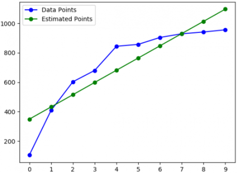
The performance of our proposed search algorithm is analysed with the different types of data sets and thoroughly compared with binary search and interpolation search algorithms. These three algorithms were implemented using Python 3.7.5 programming on AMD A9 -9420 Radeon r5 with 4GB RAM, in 64-bit Ubuntu19.10 environment. The experimentation was carried out on two different data sets: Linear and Non-liner data sets. The performance on each item in the data sets is analysed and presented in terms of the number of comparisons. The analysis of the proposed fast searching technique on linear dataset and nonlinear dataset is presented in the following Table 2 and Table 3 respectively. The graph representation of the actual data points and estimated data points of both linear data set and non-linear data set are given in Figure 2 and Figure 3 respectively.
The execution results of the proposed fast search algorithm have been compared with the execution results of binary search and interpolation search algorithms. The comparison results are presented in the following table. The average number of comparisons of the different datasets of size 10, 100, 1000, 10000, 100000 is given in Table 4. In each case, the dataset has been randomly taken between (0, 10), (0, 100), (0, 1000), (0, 10000), (0, 100000) values.
The results presented in Table 4, shows that the average number of comparisons (iterations) required for our proposed search algorithm is less than the other two cases. When the data is linear, our algorithm performs well than search on a non-linear dataset.
Figure 2. Graph representation of actual and estimated points of linear dataset
Figure 3. Graph representation of actual and estimated points of non-linear dataset
The total computation time of the proposed and the traditional methods are indicated in Figure 4. The total computation time levels of the proposed model are less that indicates the performance levels.
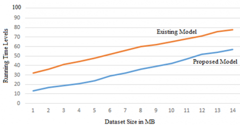
The running time of the proposed and traditional methods are indicated in Figure 5. The running time of the proposed model is less than the traditional method that indicates the performance levels are better than the existing models.
Figure 4. Total computation time levels
Figure 5. Running time levels
Table 2. Analysis of proposed search on linear dataset
|
Number of comparisons required for search of each key in Linear dataset of size n=10 |
||||||||||
|
Index |
0 |
1 |
2 |
3 |
4 |
5 |
6 |
7 |
8 |
9 |
|
Key |
105 |
409 |
603 |
680 |
844 |
857 |
904 |
929 |
941 |
956 |
|
No. of Comparisons |
1 |
2 |
2 |
1 |
2 |
2 |
1 |
2 |
2 |
3 |
Table 3. Analysis of proposed search on Non-linear dataset
|
Number of comparisons required for search of each key in Non-linear dataset of size n=10 |
||||||||||
|
Index |
0 |
1 |
2 |
3 |
4 |
5 |
6 |
7 |
8 |
9 |
|
Key |
2 |
5 |
7 |
18 |
29 |
69 |
125 |
250 |
520 |
990 |
|
No. of Comparisons |
3 |
2 |
1 |
2 |
3 |
4 |
4 |
3 |
1 |
1 |
Table 4. Comparison of binary search, interpolation search and proposed novel fast search techniques (number of iteration/comparisons)
|
Data Set Size |
Range - data Items between (min, max) |
Avg No. of comparisons in Binary Search |
Avg No. of comparisons in Interpolation Search |
Avg No. of comparisons Proposed Novel fast Search |
|
n=10 |
(0,10) |
2.1 |
1.7 |
1.2 |
|
(0, 100) |
2.9 |
2.2 |
1.7 |
|
|
(0, 1000) |
2.9 |
1.6 |
1.6 |
|
|
(0, 10000) |
2.9 |
1.8 |
1.5 |
|
|
(0, 100000) |
2.9 |
1.8 |
1.8 |
|
|
n=100 |
(0,10) |
2.9 |
1.1 |
1.2 |
|
(0, 100) |
4.8 |
1.8 |
2.1 |
|
|
(0, 1000) |
5.7 |
2.4 |
2.7 |
|
|
(0, 10000) |
5.8 |
3.1 |
3.3 |
|
|
(0, 100000) |
5.8 |
2.7 |
2.1 |
|
|
n=1000 |
(0,10) |
3.4 |
1.2 |
1.1 |
|
(0, 100) |
5.7 |
1.4 |
1.8 |
|
|
(0, 1000) |
8.2 |
3.1 |
4.6 |
|
|
(0, 10000) |
8.9 |
5.1 |
5.6 |
|
|
(0, 100000) |
8.9 |
9.2 |
5.1 |
|
|
n=10000 |
(0,10) |
2.9 |
1.3 |
1.1 |
|
(0, 100) |
5.8 |
1.4 |
1.3 |
|
|
(0, 1000) |
8.9 |
2.2 |
7.6 |
|
|
(0, 10000) |
11.5 |
3.5 |
9.4 |
|
|
(0, 100000) |
12.2 |
21.8 |
13.1 |
The novel fast search algorithm has been proposed and implemented in this work. The algorithm has been developed based on the least square regression curve fitting technique. The algorithm has been covered all the cases of the possible datasets like linear, non-linear, outliers, and zero-slope values. The experiments have been conducted with different datasets of different sizes. The performance of the proposed search algorithm has been toughly analysed and compared with the performance of the binary search and interpolation search. Experimental results have shown that the proposed novel fast searching algorithm is taking a smaller number of comparison (iterations) compared to binary search and interpolation search.
[1] Oliveira, R. (2010). Sums of random Hermitian matrices and an inequality by Rudelson. Electronic Communications in Probability, 15: 203-212. https://doi.org/10.1214/ECP.v15-1544
[2] Mehmood, T., Martens, H., Sæbø, S., Warringer, J., Snipen, L. (2011). A Partial Least Squares based algorithm for parsimonious variable selection. Algorithms for Molecular Biology, 6(1): 27. https://doi.org/10.1186/1748-7188-6-27
[3] Mehmood, T., Martens, H., Sæbø, S., Warringer, J., Snipen, L. (2011). Mining for genotype-phenotype relations in Saccharomyces using partial least squares. BMC Bioinformatics, 12(1): 318. https://doi.org/10.1186/1471-2105-12-318
[4] Mehmood, T., Liland, K.H., Snipen, L., Sæbø, S. (2012). A review of variable selection methods in partial least squares regression. Chemometrics and Intelligent Laboratory Systems, 118: 62-69. https://doi.org/10.1016/j.chemolab.2012.07.010
[5] Tran, T.N., Afanador, N.L., Buydens, L.M., Blanchet, L. (2014). Interpretation of variable importance in partial least squares with significance multivariate correlation (sMC). Chemometrics and Intelligent Laboratory Systems, 138: 153-160. https://doi.org/10.1016/j.chemolab.2014.08.005
[6] Gosselin, R., Rodrigue, D., Duchesne, C. (2010). A Bootstrap-VIP approach for selecting wavelength intervals in spectral imaging applications. Chemometrics and Intelligent Laboratory Systems, 100(1): 12-21. https://doi.org/10.1016/j.chemolab.2009.09.005
[7] Kvalheim, O.M., Rajalahti, T., Arneberg, R. (2009). X-tended target projection (XTP)-comparison with orthogonal partial least squares (OPLS) and PLS post-processing by similarity transformation (PLS+ ST). Journal of Chemometrics: A Journal of the Chemometrics Society, 23(1): 49-55. https://doi.org/10.1002/cem.1193
[8] Talukdar, U., Hazarika, S.M., Gan, J.Q. (2018). A Kernel Partial least square based feature selection method. Pattern Recognition, 83: 91-106. https://doi.org/10.1016/j.patcog.2018.05.012
[9] Mehmood, T. (2016). Hotelling T2 based variable selection in partial least squares regression. Chemometrics and Intelligent Laboratory Systems, 154: 23-28. https://doi.org/10.1016/j.chemolab.2016.03.001
[10] Cormen, T.H., Leiserson, C.E., Rivest, R.L., Stein, C. (2009). Introduction to Algorithms. MIT Press.
[11] Knuth, D.E. (1997). The Art of computer Programming (Vol. 3). Pearson Education.
[12] Van Sandt, P., Chronis, Y., Patel, J.M. (2019). Efficiently searching in-memory sorted arrays: Revenge of the interpolation search? SIGMOD '19: Proceedings of the 2019 International Conference on Management of Data, Amsterdam Netherlands, pp. 36-53. https://doi.org/10.1145/3299869.3300075
[13] https://pandas.pydata.org/pandas-ocs/stable/generated/pandas. Series.searchsorted.html, accessed on 1 November 2018.
[14] http://leveldb.org/, accessed on 1 November 2018.
[15] Perl, Y., Itai, A., Avni, H. (1978). Interpolation search-a log log N search. Communications of the ACM, 21(7): 550-553. https://doi.org/10.1145/359545.359557
[16] https://uomustansiriyah.edu.iq/media/lectures/5/5_2018_01_14!04_33_12_PM.pdf, accessed on 1 November 2018.
[17] https://sam.nitk.ac.in/courses/MA608/Curve%20Fitting.pdf, accessed on 1 November 2018.
[18] Chakrabarty, D. (2013). Curve fitting: Step-wise least squares method. Aryabhatta Journal of Mathematics & Informatics, 6(1): 15-25.
[19] Ezekiel, M., Fox, K.A. (1959). Methods of Correlation and Regression Analysis: Linear and Curvilinear. (3rd ed.). John Wiley.
[20] Bland, J.M., Altman, D. (1986). Statistical methods for assessing agreement between two methods of clinical measurement. The Lancet, 327(8476): 307-310. https://doi.org/10.1016/S0140-6736(86)90837-8