Liang Ke
© 2020 IIETA. This article is published by IIETA and is licensed under the CC BY 4.0 license (http://creativecommons.org/licenses/by/4.0/).
OPEN ACCESS
This paper probes deep into the synchronization control of high-order inertial Hopfield neural network with time delay, considering both inertia term and high-order term. Specifically, a second-order differential system was transformed into a first-order differential system, through proper variable substitution. Then, the sufficient conditions for exponential synchronization of the response system were theorized, with the aid of the fundamental solution matrix of the differential equation. The theoretical conditions were verified through an example analysis. The research findings have great application potential in production, communication, and automation.
high-order inertial Hopfield neural network, variable substitution, fundamental solution matrix, exponential synchronization
In recent years, synchronous control has been widely applied in communication, automation, and other fields. Currently, there are many effective strategies for synchronous control. In essence, synchronous control aims to synchronize the neural network, and improve the network performance. However, it is a difficult task to synchronize the neural network, which is generally a large complex nonlinear system. To solve the synchronous control problem, the key lies in the proper setting of the controller.
Compared with first-order neural network, high-order neural network boasts large capacity and strong power of approximation. The dynamic properties of high-order neural network have attracted much attention from the academia. For instance, Zhang [1] probed deep into pseudo almost periodic high-order cellular neural networks with complex deviating arguments. Alim et al. [2] explored the dynamics and oscillations of generalized high-order Hopfield neural networks with mixed delays. Aouiti [3] investigated the oscillation of generalized high-order Hopfield neural networks with impulsive neutral delay. Zhao et al. [4] discussed the weighted pseudo-almost automorphic solutions of high-order Hopfield neural networks with neutral distributed delays. Wang and Rathinasamy [5] examined double almost periodicity for high-order Hopfield neural networks with slight vibration in time variables. Huang et al. [6] and He et al. [7] studied the asymptotical stability and global exponential stability of high-order neutral neural networks, respectively. Dong et al. [8] measured the global exponential stability of higher-order delayed discrete-time Cohen-Grossberg neural networks based on a nonsingular M-matrix. Arbi et al. [9] analyzed the stability of delayed high-order Hopfield neural networks with impulses. Xu and Wu [10] searched for anti-periodic solutions of high-order cellular neural networks with mixed delays and impulses.
In the above studies, the damping coefficient of the neural network does not include inertia. From the perspectives of mathematics and physics, a neural network can be understood as a super model of infinitely large damping. But the dynamic properties of each neuron will change, once the inertia exceeds the critical value. In practice, many scholars have considered the dynamic properties of the system with weak damping, that is, the dynamic behaviors of neural network with inertia terms [11-18]. For example, Pecora and Carroll [19] put forward the concept of power system synchronization: the drive system (controlling neural network) and response system (controlled neural network) are synchronized, when the two systems have the same structure and parameters.
Synchronization has been extensively applied in neural network, which stimulates the research into the synchronization stability of inertial neural network. Using variable transform and Lyapunov-Krasovskii functionals, Wan et al. [20] realized the global exponential synchronization of inertial reaction-diffusion coupled neural networks with proportional delay. Xiao et al. [21] achieved the global exponential synchronization of generalized discrete-time inertial neural networks. Based on the properties of Riemann-Liouville fractional derivative, Gu et al. [22] tackled the stability and synchronization of inertial neural networks with Riemann-Liouville fractional-order delay through variable substitution. By integral inequality method, Zhang and Cao [23] constructed Lyapunov function, and provided the sufficient condition of finite-time synchronization for inertial neural networks with time delays. Tang and Jian [24] solved the exponential synchronization of inertial neural networks with periodic intermittent control and hybrid variable delay. With the aid of integral inequality, Zhang and Ren [25] came up with the new sufficient conditions for global asymptotic synchronization of inertial delayed neural networks. Ke and Li [26, 27] provided the sufficient conditions for exponential synchronization of inertial neural networks and inertial Cohen-Grossberg neural networks. Brahmi et al. [28] explored the exponential synchronization of high-order Hopfield neural networks. Li et al. [29] considered the almost automorphic synchronization of quaternion-valued high-order Hopfield neural networks. None of the above studies have discussed the synchronization stability of high-order inertial Hopfield neural networks.
To sum up, the inertia term [21-27] and high-order term [28] have not been considered simultaneously in the previous research on the exponential synchronization of neural network. To make up for the gap, this paper explores the exponential synchronization of high-order inertial of Hopfield neural networks with time delay. Both inertia and high-order terms were investigated through innovative derivation method, producing novel results.
The remainder of this paper is organized as follows: Section 2 formulates the neural network model, and gives some preliminaries; Section 3 presents the main results of exponential synchronization; Section 4 proves the effectiveness of our synchronization strategy through example analysis; Section 5 puts forward the conclusions.
The high-order inertia Hopfield neural network with time delay can be formulated as:
$\frac{d^{2} x_{i}(t)}{d t^{2}}=-\beta_{i} \frac{d x_{i}(t)}{d t}-\alpha_{i} x_{i}(t)$
$+\sum_{j=1}^{n} a_{i j} f_{j}\left(x_{j}(t)\right)+\sum_{j=1}^{n} b_{i j} f_{j}\left(x_{j}\left(t-\tau_{i j}\right)\right)$
$+\sum_{j=1}^{m} \sum_{k=1}^{m} c_{i j k} f_{j}\left(x_{j}\left(t-\tau_{i j}\right)\right) f_{k}\left(x_{k}\left(t-\tau_{i k}\right)\right)+I_{i}$ (1)
where, i=1, 2, ···, n; αi and βj>0 are constants; xi(t) is the state variable of the i-th neuron; bijand cijare connection weights; fj is the activation function; τij is time delay; Iiis the input to the i-th neuron at time t.
The initial conditions of system (1) can be expressed as:
$x_{i}(s)=\varphi_{x i}(s), \frac{d x_{i}(s)}{d t}=\psi_{x i}(s),-\tau \leq s \leq 0$ (2)
where, $\tau=\max _{1 \leq i, j \leq n}\left\{\tau_{i j}\right\}$ , φxi(s), and ψxi(s) are bounded and continuous functions.
The response system corresponding to system (1) can be described as:
$\frac{d^{2} y_{i}(t)}{d t^{2}}=-\beta_{i} \frac{d y_{i}(t)}{d t}-\alpha_{i} y_{i}(t)$
$+\sum_{j=1}^{n} a_{i j} f_{j}\left(y_{j}(t)\right)+\sum_{j=1}^{n} b_{i j} f_{j}\left(y_{j}\left(t-\tau_{i j}\right)\right)$
$+\sum_{j=1}^{m} \sum_{k=1}^{m} c_{i j k} f_{j}\left(y_{j}\left(t-\tau_{i j}\right)\right) f_{k}\left(y_{k}\left(t-\tau_{i k}\right)\right)+u_{i}(t)+I_{i}$ (3)
where, ui(t) is the feedback controller; i=1, 2, ..., n.
The initial values of the response system (3) can be defined as:
$y_{i}(s)=\varphi_{y i}(s), \frac{d y_{i}(s)}{d t}=\psi_{y i}(s),-\tau \leq s \leq 0$ (4)
here, φyi(s) and ψyi(s) are bounded and continuous functions.
Then, the following hypothesis was put forward:
Hypothesis: Activation function fjis differentiable on xiand in line with Lipschitz condition, and there exists a constant lj>0 making: $\left.\mid f_{j}\left(v_{1}\right)-f_{j}\left(v_{2}\right)\right)\left|\leq l_{j}\right| v_{1}-v_{2} \mid, v_{1}, v_{2} \in \Re, j=1,2, \ldots, n$.
Definition 1. For systems (1) and (3), if there exist constants λ>0 and c>0, such that: $\| x(t)-y\left(t \|=\sum_{i=1}^{n}\left|x_{i}(t)-y_{i}(t)\right| \leq c e^{-\lambda\left(t-t_{0}\right)}\right.$, t>t0.
Then, systems (1) and (3) are exponentially synchronized.
Lemma 1. [30] Suppose a>b>0. If function x(t) is non-negative and continuous in [t0-µ, t], and satisfies the following inequalities in the interval: $D^{+} x(t) \leq-a x(t)+b \bar{x}(t)$. Then, $x(t) \leq \bar{x}\left(t_{0}\right) e^{-\lambda\left(t-t_{0}\right)}$, t≥t0. where, $\bar{x}(t)=\sup _{t-\mu \leq s \leq t}\{x(s)\}$, μ≥0 is a constant; λ is the unique positive root of transcendental equation λ=a−beλt.
Lemma 2. [31] For (x1(t), x2(t), ..., xm(t))T, $\left(x_{1}^{*}(t), x_{2}^{*}(t), \cdots, x_{m}^{*}(t)\right)^{T} \in R^{m}$, if hj(xj) is continuously differentiable in xj (j=1, 2, …, m). then: $\sum_{j=1}^{m} \sum_{k=1}^{m} b_{i j k}\left[h_{j}\left(x_{j}\right) h_{k}\left(x_{k}\right)-h_{j}\left(x_{j}^{*}\right) h_{k}\left(x_{k}^{*}\right)\right]= \sum_{j=1}^{m} \sum_{k=1}^{m}\left(b_{i j k}+b_{i k j}\right)\left[h_{j}\left(x_{j}\right)-h_{j}\left(x_{j}^{*}\right)\right] h_{k}\left(\xi_{k}\right)$. where, ξk is a value between xk and $x_{k}^{*}$; j, k=1, 2, ..., m.
Through proper variable substitution, this section transforms a second-order differential system into a first-order differential system, and thus derives the sufficient conditions for exponential synchronization of the response system (3) with the drive system (1).
The variable substitution can be expressed as: $z_{i}(t)=\dot{x}_{l}(t)+\eta_{i} x_{i}(t), w_{i}(t)=\dot{y}_{i}(t)+\eta_{i} y_{i}(t)$, ηi>0, i=1, 2, …, m.
Then, systems (1) and (3) can be rewritten as:
$\left\{\begin{array}{c}\dot{x}_{i}(t)=-\eta_{i} x_{i}(t)+z_{i}(t) \\ \dot{z}_{l}(t)=\left(\beta_{i} \eta_{i}-\alpha_{i}-\eta_{i}^{2}\right) x_{i}(t) \\ +\left(\eta_{i}-\beta_{i}\right) z_{i}(t)+\sum_{j=1}^{n} a_{i j} f_{j}\left(x_{j}(t)\right. \\ +\sum_{j=1}^{n} b_{i j} f_{j}\left(x_{j}\left(t-\tau_{i j}\right)\right) \\ +\sum_{j=1}^{n} \sum_{k=1}^{n} c_{i j k} f_{j}\left(x_{j}\left(t-\tau_{i j}\right)\right) f_{k}\left(x_{k}\left(t-\tau_{j k}\right)\right)+I_{i}\end{array}\right.$ (5)
$\left\{\begin{array}{c}\dot{y}_{i}(t)=-\eta_{i} y_{i}(t)+w_{i}(t) \\ \dot{w}_{l}(t)=\left(\beta_{i} \eta_{i}-\alpha_{i}-\eta_{i}^{2}\right) y_{i}(t)+\left(\eta_{i}-\beta_{i}\right) w_{i}(t) \\ +\sum_{j=1}^{n} a_{i j} f_{j}\left(y_{j}(t)\right)+\sum_{j=1}^{n} b_{i j} f_{j}\left(y_{j}\left(t-\tau_{i j}\right)\right) \\ +\sum_{j=1}^{m} \sum_{k=1}^{m} c_{i j k} f_{j}\left(y_{j}\left(t-\tau_{i j}\right)\right) f_{k}\left(y_{k}\left(t-\tau_{i k}\right)\right)+u_{i}(t)+I_{i}\end{array}\right.$ (6)
The error can be described as: e1i(t)=yi(t)-xi(t), e2i(t)=wi(t)-zi(t), i=1, 2, …, n.
By Lemma 2, the following can be derived from formulas (5) and (6):
$\left\{\begin{array}{c}e_{1_{l}}^{.}(t)=-\eta_{i} e_{1 i}(t)+e_{2 i}(t) \\ e_{2 \iota}^{.}(t)=\left(\eta_{i} \beta_{i}-\alpha_{i}-\eta_{i}^{2}\right) e_{1 i}(t) \\ +\left(\eta_{i}-\beta_{i}\right) e_{2 i}(t)+\sum_{j=1}^{n} a_{i j} \bar{f}_{j}\left(e_{1 j}(t)\right) \\ +\sum_{j=1}^{m}\left[b_{i j}+\sum_{k=1}^{n}\left(c_{i j k}+c_{i k j}\right)\right] \bar{f}_{j}\left(e_{1 j}\left(t-\tau_{i j}\right)\right)+u_{i}(t)\end{array}\right.$ (7)
where, $\bar{f}_{j}\left(e_{1 j}(t)\right)=f_{j}\left(y_{j}(t)\right)-f_{j}\left(x_{j}(t)\right)$; j=1, 2, ..., n.
Theorem 1. If the Hypothesis holds for the following feedback controller: ui(t)=-λie1i(t), i=1, 2, ..., n.
If $\beta_{i}-\sqrt{\left|\beta_{i}^{2}-4\left(\alpha_{i}+\lambda_{i}\right)\right|}>0$, and σ- $\max _{1 \leq i \leq n}\left\{M\left[\sum_{j=1}^{n}\left|a_{j i}\right| l_{i}+\sum_{j=1}^{n}\left|b_{j i}+\sum_{k=1}^{n}\left(c_{j i k}+c_{j k i}\right)\right| l_{i}\right\}>0\right.$, then systems (1) and (3) are exponentially synchronized. where, $\sigma=\min _{1 \leq i \leq n}\left\{\frac{\beta_{i}-\sqrt{\mid\left(\beta_{i}^{2}-4\left(\alpha_{i}+\lambda_{i}\right) \mid\right.}}{2}, \frac{\beta_{i}}{2}\right\}$, $M=\max _{1 \leq i \leq n}\left\{\frac{2\left(1+\beta_{i}+\left|\eta_{i} \beta_{i}-\alpha_{i}-\eta_{i}^{2}-\lambda_{i}\right|+\sqrt{\left|\beta_{i}^{2}-4\left(\alpha_{i}+\lambda_{i}\right)\right|}\right)}{\sqrt{\left|\beta_{i}^{2}-4\left(\alpha_{i}+\lambda_{i}\right)\right|}}\right\}$.
Proof.
Let $D_{i}=\left[\begin{array}{cc}\eta_{i} & -1 \\ \alpha_{i}+\eta_{i}^{2}+\lambda_{i}-\eta_{i} \beta_{i} & \beta_{i}-\eta_{i}\end{array}\right]$ and $E_{i}(t)=\left[\begin{array}{l}e_{1 i}(t) \\ e_{2 i}(t)\end{array}\right]$, $F_{i}(t)=\left[\begin{array}{c}0 \\ \bar{f}_{j}\left(e_{1 j}(t)\right)\end{array}\right]$.
From formula (7), it can be derived that:
$\frac{d E_{i}(t)}{d t}=-D_{i} E_{i}(t)+\sum_{j=1}^{n} a_{i j} F_{i}(t)$
$+\sum_{j=1}^{n}\left[b_{i j}+\sum_{k=1}^{n}\left(c_{i j k}+c_{i k j}\right)\right] F_{i}\left(t--\tau_{i j}\right)$ (8)
For the following linear differential equation:
$W^{\prime}(t)=-D_{i} W(t)$ (9)
The eigenvalues of −Di can be obtained: $\xi_{1}=\frac{-\beta_{i}+\sqrt{\beta_{i}^{2}-4\left(\alpha_{i}+\lambda_{i}\right)}}{2}, \xi_{2}=\frac{-\beta_{i}-\sqrt{\beta_{i}^{2}-4\left(\alpha_{i}+\lambda_{i}\right)}}{2}$.
The corresponding eigenvectors are: V1=(1, ξ1+ηi)T, V2=(1, ξ2+ηi)T.
Thus, the fundamental solution matrix of system (9) can be obtained as: $\phi(t)=\left[\begin{array}{cc}e^{\xi_{1} t} & e^{\xi_{2} t} \\ \left(\xi_{1}+\eta_{i}\right) e^{\xi_{1} t} & \left(\xi_{2}+\eta_{i}\right) e^{\lambda_{2} t}\end{array}\right]$.
If $\beta_{i}^{2}-4\left(\alpha_{i}+\lambda_{i}\right) \neq 0$, then: $\phi^{-1}(0)=\frac{1}{\lambda_{2}-\lambda_{1}}\left[\begin{array}{cc}\xi_{2}+\eta_{i} & -1 \\ -\left(\xi_{1}+\eta_{i}\right) & 1\end{array}\right]$.
Since e-Dit=ϕ(t)ϕ-1(0), we have:
$e^{-D_{i} t}$=$\frac{1}{\xi_{2}-\xi_{1}}\left[\begin{array}{cc}\left(\xi_{2}+\eta_{i}\right) e^{\xi_{1} t}-\left(\xi_{1}+\eta_{i}\right) e^{\xi_{2} t} & e^{\xi_{2} t}-e^{\xi_{1} t} \\ \left(\xi_{1}+\eta_{i}\right)\left(\xi_{2}+\eta_{i}\right)\left(e^{\xi_{1} t}-e^{\xi_{2} t}\right) & \left(\xi_{2}+\eta_{i}\right) e^{\xi_{2} t}-\left(\xi_{1}+\eta_{i}\right) e^{\xi_{1} t}\end{array}\right]$.
If $\beta_{i}^{2}-4\left(\alpha_{i}+\lambda_{i}\right)>0$, then
$\left\|e^{-D_{i} t}\right\|\leq \frac{2\left(1+\beta_{i}+\left|\eta_{i} \beta_{i}-\alpha_{i}-\eta_{i}^{2}-\lambda_{i}\right|+\sqrt{\beta_{i}^{2}-4\left(\alpha_{i}+\lambda_{i}\right)}\right.}{\sqrt{\beta_{i}^{2}-4\left(\alpha_{i}+\lambda_{i}\right)}} e^{-\frac{\beta_{i}-\sqrt{\beta_{i}^{2}-4\left(\alpha_{i}+\lambda_{i}\right)}}{2} t}$
If $\beta_{i}^{2}-4\left(\alpha_{i}+\lambda_{i}\right)<0$, then
$\left\|e^{-D_{i} t}\right\|\leq \frac{2\left(1+\beta_{i}+\left|\eta_{i} \beta_{i}-\alpha_{i}-\eta_{i}^{2}-\lambda_{i}\right|+\sqrt{\left|\beta_{i}^{2}-4\left(\alpha_{i}+\lambda_{i}\right)\right|}\right.}{\sqrt{\left|\beta_{i}^{2}-4\left(\alpha_{i}+\lambda_{i}\right)\right|}} e^{-\frac{\beta_{i}}{2} t}$
Thus, if $\beta_{i}^{2}-4\left(\alpha_{i}+\lambda_{i}\right) \neq 0$, then $\left\|e^{-D_{i} t}\right\| \leq M e^{-\sigma t}$, t>0, where,
$\sigma=\min _{1 \leq \mathrm{i} \leq \mathrm{n}}\left\{\frac{\beta_{\mathrm{i}}-\sqrt{\left|\beta_{\mathrm{i}}^{2}-4\left(\alpha_{\mathrm{i}}+\lambda_{\mathrm{i}}\right)\right|}}{2}, \frac{\beta_{\mathrm{i}}}{2}\right\}$;
$M=\max _{1 \leq i \leq n}\left\{\frac{2\left(1+\beta_{i}+\left|\eta_{i} \beta_{i}-\alpha_{i}-\eta_{i}^{2}-\lambda_{i}\right|+\sqrt{\left|\beta_{i}^{2}-4\left(\alpha_{i}+\lambda_{i}\right)\right|}\right.}{\sqrt{\left|\beta_{i}^{2}-4\left(\alpha_{i}+\lambda_{i}\right)\right|}}\right\}$.
From formula (8), we have:
$e^{D_{i} t}\left[\frac{d E_{i}(t)}{d t}+D E_{i}(t)\right]=e^{D_{i} t} \sum_{j=1}^{n} a_{i j} F_{i}(t)$
$+\sum_{j=1}^{n}\left[b_{i j}+\sum_{k=1}^{n}\left(c_{i j k}+c_{i k j}\right)\right] F_{i}\left(t-\tau_{i j}\right)$ (10)
From formula (10), we have:
$E_{i}(t)=e^{-D_{i} t} E_{i}(0)$
$+\int_{0}^{t} e^{-D_{i}(t-s)}\left\{\sum_{j=1}^{n} a_{i j} F_{j}(s)+\sum_{j=1}^{n}\left[b_{i j}+\sum_{k=1}^{n}\left(c_{i j k}+c_{i k j}\right)\right] F_{j}\left(s-\tau_{i j}\right) d s .\right\}$ (11)
And
$\left\|E_{i}(t)\right\| \leq\left\|e^{-D_{i} t} E_{i}(0)\right\|+\int_{0}^{t}\left\|e^{-D_{i}(t-s)}\right\|\left\{\sum_{j=1}^{n}\left|a_{i j}\right| \|\right.$
$\left.F_{j}(s)\left\|+\sum_{j=1}^{n}\left|b_{i j}+\sum_{k=1}^{n}\left(c_{i j k}+c_{i k j}\right)\right|\right\| F_{j}\left(s-\tau_{i j}\right) \|\right\} d s$
$\leq M e^{-\sigma t}\left\|E_{i}(0)\right\|+M \int_{0}^{t} e^{-\sigma(t-s)}\left\{\sum_{j=1}^{n}\left|a_{i j}\right| l_{j}\left|e_{1 j}(s)\right|+\right.$
$\left.\sum_{j=1}^{n}\left|b_{i j}+\sum_{k=1}^{n}\left(c_{i j k}+c_{i k j}\right)\right| l_{j} \mid e_{1 j}\left(s-\tau_{i j}\right)\right\} d s \leq$
$M e^{-\sigma t}\left\|E_{i}(0)\right\|+M \int_{0}^{t} e^{-\sigma(t-s)}\left\{\sum_{j=1}^{n}\left|a_{i j}\right| l_{j}\left|E_{j}(s)\right|+\right.$
$\left.\sum_{j=1}^{n}\left|b_{i j}+\sum_{k=1}^{n}\left(c_{i j k}+c_{i k j}\right)\right| l_{j} \mid E_{j}\left(s-\tau_{i j}\right)\right\} d s$.
Let
$p_{i}(t)=M e^{-\sigma t}\left\|E_{i}(0)\right\|$
$\left.+M \int_{0}^{t} e^{-\sigma(t-s)\left\{\sum_{j=1}^{n}\left|a_{i j}\right| l_{j} \| E_{j}(s)\right.}\left\|+\sum_{j=1}^{n}\left|b_{i j}+\sum_{k=1}^{n}\left(c_{i j k}+c_{i k j}\right)\right| l_{j}\right\| E_{j}\left(s-\tau_{i j}\right) \|\right\} d s$,
$t>0, p_{i}(t)=M\left\|E_{i}(t)\right\|,-\tau \leq t \leq 0$. (12)
where, $\left\|\bar{E}_{i}(t)\right\|=\sup _{t-\tau \leq s \leq t}\left\|E_{i}(t)\right\|$, $\left\|\bar{p}_{i}(t)\right\|=\sup _{t-\tau \leq s \leq t}\left\|p_{i}(t)\right\|$. It can be derived that $p_{i}(t) \geq\left\|E_{i}(t)\right\|, \bar{p}_{i}(t) \geq\left\|\bar{E}_{i}(t)\right\|$.
Solving the upper right Dini derivative D+pi(t) of pi(t):
$D^{+} p_{i}(t)=-\sigma p_{i}(t)+M\left\{\sum_{j=1}^{n}\left|a_{i j}\right| l_{j}\left\|E_{j}(t)\right\|\right.$
$\left.+\sum_{j=1}^{n}\left|b_{i j}+\sum_{k=1}^{n}\left(c_{i j k}+c_{i k j}\right)\right| l_{j}\left\|E_{j}\left(t-\tau_{i j}\right)\right\|\right\} \leq$
$-\sigma p_{i}(t)+M\left\{\sum_{j=1}^{n}\left|a_{i j}\right| l_{j}+\sum_{j=1}^{n} \mid b_{i j}+\sum_{k=1}^{n}\left(c_{i j k}+\right.\right.$
$\left.\left.c_{i k j}\right) \mid l_{j} \bar{p}_{j}(t)\right\}$.
Let $p(t)=\sum_{i=1}^{n} p_{i}(t)$. From the above, it can be obtained that
$D^{+} p(t) \leq \sum_{i=1}^{n}\left\{-\sigma p_{i}(t)+M\left[\sum_{j=1}^{n}\left|a_{i j}\right| l_{j}+\sum_{j=1}^{n} \mid b_{i j}+\right.\right.$
$\left.\left.\sum_{k=1}^{n}\left(c_{i j k}+c_{i k j}\right) \mid l_{j} \bar{p}_{j}(t)\right] \leq-\sigma p(t)+N \bar{p}(t)\right\}$,
where $N=\max _{1 \leq i \leq n}\left\{M\left[\sum_{j=1}^{n}\left|a_{j i}\right| l_{i}+\sum_{j=1}^{n} \mid b_{j i}\right.\right.$+ $\left.\sum_{k=1}^{n} \left(c_{j i k}+c_{j k i}\right) \mid l_{i}\right\}$.
Since $\sigma-\max _{1 \leq i \leq n}\left\{M\left[\sum_{j=1}^{n}\left|a_{j i}\right| l_{i}+\sum_{j=1}^{n}\left|b_{j i}+\sum_{k=1}^{n} \left(c_{j i k}+c_{j k i}\right)\right| l_{i}\right\}>0\right.$, by Lemma 1,
$\mathrm{p}(\mathrm{t}) \leq \overline{\mathrm{p}}(0) \mathrm{e}^{-\xi \mathrm{t}}, \mathrm{t} \geq 0$ (13)
where, ξ is the positive root of equation ξ=σ-Neξt.
From formula (13), we have $\| x(t)-y\left(t \|=\sum_{i=1}^{n}\left|x_{i}(t)-y_{i}(t)\right| \leq c e^{-\xi t}\right.$, ξ>0, t>0, where, $c=M \sum_{i=1}^{n}\left[\left|\psi_{y i}(0)-\varphi_{x i}(0)\right|+\left|\psi_{y i}(0)+\eta_{i} \varphi_{y i}(0)-\psi_{x i}(0)-\eta_{i} \varphi_{x i}(0)\right|\right]$.
By Definition 1, systems (1) and (3) are exponentially synchronized.
If cijk=0, i, j, k=1, 2, ..., m, then system (1) becomes an inertial neural network with time delay:
$\frac{d^{2} x_{i}(t)}{d t^{2}}=-\beta_{i} \frac{d x_{i}(t)}{d t}-\alpha_{i} x_{i}(t)+\sum_{j=1}^{n} a_{i j} f_{j}\left(x_{j}(t)\right)$
$+\sum_{j=1}^{n} b_{i j} f_{j}\left(x_{j}\left(t-\tau_{i j}\right)\right)$ (14)
The corresponding response system can be represented as:
$\frac{d^{2} y_{i}(t)}{d t^{2}}=-\beta_{i} \frac{d y_{i}(t)}{d t}-\alpha_{i} y_{i}(t)+\sum_{j=1}^{n} a_{i j} f_{j}\left(y_{j}(t)\right)$
$+\sum_{j=1}^{n} b_{i j} f_{j}\left(y_{j}\left(t-\tau_{i j}\right)\right)$. (15)
where, ui(t) is the feedback controller; i=1, 2, ..., n.
The following corollary can be obtained from Theorem 1.
Corollary 1. Suppose the Hypothesis holds for the following feedback controller: ui(t)=-λie1i(t), i=1,2, ..., n.
If $\beta_{i}-\sqrt{\left|\beta_{i}^{2}-4\left(\alpha_{i}+\lambda_{i}\right)\right|}>0$, and $\sigma-\max _{1 \leq i \leq n}\left\{M\left[\sum_{j=1}^{n}\left|a_{j i}\right| l_{i}+\sum_{j=1}^{n}\left|b_{j i}\right|\right\}>0\right.$,
Then, systems (14) and (15) are exponentially synchronized, where: $\sigma=\min _{1 \leq i \leq n}\left\{\frac{\beta_{i}-\sqrt{\mid\left(\beta_{i}^{2}-4\left(\alpha_{i}+\lambda_{i}\right) \mid\right.}}{2}, \frac{\beta_{i}}{2}\right\}$, $M=\max _{1 \leq i \leq n}\left\{\frac{2\left(1+\beta_{i}+\left|\eta_{i} \beta_{i}-\alpha_{i}-\eta_{i}^{2}-\lambda_{i}\right|+\sqrt{\left|\beta_{i}^{2}-4\left(\alpha_{i}+\lambda_{i}\right)\right|}\right)}{\sqrt{\left|\beta_{i}^{2}-4\left(\alpha_{i}+\lambda_{i}\right)\right|}}\right\}$.
This section illustrates the effectiveness of the above results with an example:
Example: The high-order inertial Hopfield neural network with time delay can be described as: (n=2)
$\ddot{x}_{1}(\mathrm{t})=-\beta_{\mathrm{i}} \dot{\mathrm{x}}_{\mathrm{l}}(\mathrm{t})-\alpha_{\mathrm{i}} \mathrm{x}_{\mathrm{i}}(\mathrm{t})$
$+\sum_{\mathrm{j}=1}^{2} \mathrm{a}_{\mathrm{ij}} \mathrm{f}_{\mathrm{j}}\left(\mathrm{x}_{\mathrm{j}}(\mathrm{t})\right)+\sum_{\mathrm{j}=1}^{2} \mathrm{~b}_{\mathrm{ij}} \mathrm{f}_{\mathrm{j}}\left(\mathrm{x}_{\mathrm{j}}\left(\mathrm{t}-\mathrm{\tau}_{\mathrm{ij}}\right)\right)$
$+\sum_{\mathrm{j}=1}^{2} \sum_{\mathrm{k}=1}^{2} \mathrm{c}_{\mathrm{ijk}} \mathrm{f}_{\mathrm{j}}\left(\mathrm{x}_{\mathrm{j}}\left(\mathrm{t}-\mathrm{\tau}_{\mathrm{ij}}\right)\right) \mathrm{f}_{\mathrm{k}}\left(\mathrm{x}_{\mathrm{k}}\left(\mathrm{t}-\tau_{\mathrm{jk}}\right)\right)+\mathrm{I}_{\mathrm{i}}$ (16)
The response system driven system (14) can be described as:
$\ddot{y}_{l}(t)=-\beta_{i} \dot{y}_{l}(t)-\alpha_{\mathrm{i}} \mathrm{y}_{\mathrm{i}}(\mathrm{t})$
$+\sum_{\mathrm{j}=1}^{2} \mathrm{a}_{\mathrm{ij}} \mathrm{f}_{\mathrm{j}}\left(\mathrm{y}_{\mathrm{j}}(\mathrm{t})\right)+\sum_{\mathrm{j}=1}^{2} \mathrm{~b}_{\mathrm{ij}} \mathrm{f}_{\mathrm{j}}\left(\mathrm{y}_{\mathrm{j}}\left(\mathrm{t}-\mathrm{\tau}_{\mathrm{ij}}\right)\right)$
$+\sum_{\mathrm{j}=1}^{2} \sum_{\mathrm{k}=1}^{2} \mathrm{c}_{\mathrm{ij} \mathrm{k}} \mathrm{f}_{\mathrm{j}}\left(\mathrm{y}_{\mathrm{j}}\left(\mathrm{t}-\tau_{\mathrm{ij}}\right)\right) \mathrm{f}_{\mathrm{k}}\left(\mathrm{y}_{\mathrm{k}}\left(\mathrm{t}-\tau_{\mathrm{jk}}\right)\right)+\mathrm{u}_{\mathrm{i}}(\mathrm{t})$
$+\mathrm{I}_{\mathrm{i}}$ (17)
where, ui(t)=-λi(yi(t)-xi(t)), λi>0, i=1, 2.
The relevant parameters were configured as follows: λ1=1.2, λ2=1.5, η1=1.1, η2=1.15, β1=4, β2=4.5, α1=1.45, α2=1.4, a11=0.01, a2=0.02, a21=-0.01,a22=0.03, b11=0.02, b12=-0.02, b21=0.01, b22=0.03, c111=0.01, c121=0.02, c112=0.03, c122=-0.01, c211=-0.02, c221=0.025, c212=0.015, c222=-0.025, I1=0.5, I2=0.45, τ11=0.2, τ12=0.3, τ21=0.25, and τ22=0.46, $f_{i}\left(x_{i}(t)\right)=\frac{1}{2} \cos \left(x_{i}(t)\right)$, i=1, 2.
Obviously, $\left|f_{i}\left(x_{i}\right)-f_{i}\left(y_{i}\right)\right| \leq \frac{1}{2}\left|x_{i}-y_{i}\right|, l_{i}=\frac{1}{2}$.
By simple calculation, we have:
$\beta_{1}-\sqrt{\left|\beta_{1}^{2}-4\left(\alpha_{1}+\lambda_{1}\right)\right|}=1.676209992$,
$\beta_{2}-\sqrt{\left|\beta_{2}^{2}-4\left(\alpha_{2}+\lambda_{2}\right)\right|}=1.558911766$,
$\sigma=\min _{1 \leq i \leq 2}\left\{\frac{\beta_{i}-\sqrt{\left|\beta_{i}^{2}-4\left(\alpha_{i}+\lambda_{i}\right)\right|}}{2}, \frac{\beta_{i}}{2}\right\}=0.779455883$,
$M=\max _{1 \leq i \leq 2}\left\{\frac{2\left(1+\beta_{i}+\left|\eta_{i} \beta_{i}-\alpha_{i}-\eta_{i}^{2}-\lambda_{i}\right|+\sqrt{\mid \beta_{i}^{2}-4\left(\alpha_{i}+\lambda_{i}\right)} \mid\right.}{\sqrt{\left|\beta_{i}^{2}-4\left(\alpha_{i}+\lambda_{i}\right)\right|}}\right\}=6.76807283$.
$\sigma-\max _{1 \leq i \leq n}\left\{M\left[\sum_{j=1}^{n}\left|a_{j i}\right| l_{i}+\sum_{j=1}^{n}\left|b_{j i}+\sum_{k=1}^{n}\left(c_{j i k}+c_{j k i}\right)\right| l_{i}\right\}=0.37337151327>0\right.$.
System (16) satisfies the condition of Theorem 1, indicating that systems (16) and (17) are exponentially synchronized.
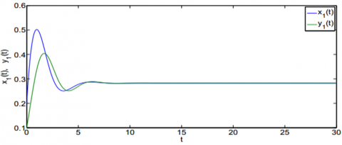
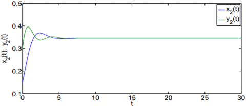
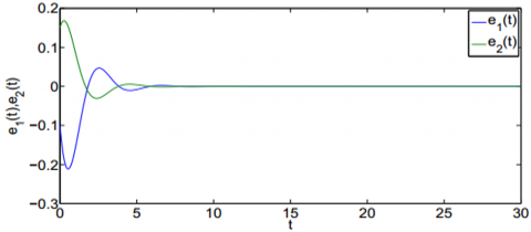
Figures 1-3 were obtained through numerical simulation. It can be seen that the simulation results are consistent with Theorem 1.
Figure 1. The synchronization trajectories between state x1(t) of the drive system (16) and state y1(t) of the response system (17)
Figure 2. The synchronization trajectories between state x2(t) of the drive system (16) and state y2(t) of the response system (17)
Figure 3. The evolution of synchronization errors e1(t) and e2(t) in the example1
This paper mainly discusses the exponential synchronization of high-order inertial neural networks with time delay, and gives two sufficient conditions for the exponential synchronization of between drive system (1) and response system (3). The research results are summarized in the form of Theorem 1.
On the exponential synchronization of neural networks, the previous studies [20-31] either evaluate the synchronization stability of inertial neural networks or that of high-order neural networks. The inertia item complicates the dynamic features of the neural network, while the high-order term induces bifurcation and chaos. In other words, the inertia term and high-order term have never been discussed at the same time, despite their significant impacts on neural network. This paper looks at both inertia term and high-order term. The combination between the two terms in neural network enriches and improves the existing neural networks. The synchronization of high-order inertial neural networks has great application potential in production, communication, and automation.
The research results provide a theoretical criterion for exploring system design and realizing practical application. Drawing on our results, the future research could tackle the synchronization of other high-order inertial neural networks with time delay, such as high-order inertial bidirectional associative memory (BAM) neural network and high-order inertial Cohen-Grossberg neural networks.
This research was funded by The National Key Technology R&D Program (Grant No.: 2013BAG19B01).
[1] Zhang, A. (2019). Pseudo almost periodic high-order cellular neural networks with complex deviating arguments. International Journal of Machine Learning and Cybernetics, 10(2): 301-309. https://doi.org/10.1007/s13042-017-0715-3
[2] Alimi, A.M., Aouiti, C., Chérif, F., Dridi, F., M’hamdi, M.S. (2018). Dynamics and oscillations of generalized high-order Hopfield neural networks with mixed delays. Neurocomputing, 321: 274-295. https://doi.org/10.1016/j.neucom.2018.01.061
[3] Aouiti, C. (2018). Oscillation of impulsive neutral delay generalized high-order Hopfield neural networks. Neural Computing and Applications, 29(9): 477-495. https://doi.org/10.1007/s00521-016-2558-3
[4] Zhao, L., Li, Y., Li, B. (2018). Weighted pseudo-almost automorphic solutions of high-order Hopfield neural networks with neutral distributed delays. Neural Computing and Applications, 29(7): 513-527. https://doi.org/10.1007/s00521-016-2553-8
[5] Wang, C., Rathinasamy, S. (2018). Double almost periodicity for high-order Hopfield neural networks with slight vibration in time variables. Neurocomputing, 282: 1-15. https://doi.org/10.1016/j.neucom.2017.12.008
[6] Huang, C., Su, R., Cao, J., Xiao, S. (2020). Asymptotically stable high-order neutral cellular neural networks with proportional delays and D operators. Mathematics and Computers in Simulation, 171: 127-135. https://doi.org/10.1016/j.matcom.2019.06.001
[7] He, Z.L., Li, C.D., Li, H.F., Zhang, Q. (2020). Global exponential stability of high-order Hopfield neural networks with stated pendent impulses. Physica A: Statistical Mechanics and its Applications, 542: 123434. https://doi.org/10.1016/j.physa.2019.123434
[8] Dong, Z., Wang, X., Zhang, X. (2020). A nonsingular M-matrix-based global exponential stability analysis of higher-order delayed discrete-time Cohen–Grossberg neural networks. Applied Mathematics and Computation, 385: 125401. https://doi.org/10.1016/j.amc.2020.125401
[9] Arbi, A., Aouiti, C., Chérif, F., Touati, A., Alimi, A.M. (2015). Stability analysis for delayed high-order type of Hopfield neural networks with impulses. Neurocomputing, 165: 312-329. https://doi.org/10.1016/j.neucom.2015.03.021
[10] Xu, C., Wu, Y. (2015). Anti-periodic solutions for high-order cellular neural networks with mixed delays and impulses. Advances in Difference Equations, 2015(1): 1-14.
[11] Huo, N., Li, B., Li, Y. (2019). Existence and exponential stability of anti-periodic solutions for inertial quaternion-valued high-order Hopfield neural networks with state-dependent delays. IEEE Access, 7: 60010-60019. https://doi.org/10.1109/ACCESS.2019.2915935
[12] Ke, Y., Miao, C. (2017). Anti-periodic solutions of inertial neural networks with time delays. Neural Processing Letters, 45(2): 523-538. https://doi.org/10.1007/s11063-016-9540-z
[13] Wan, P., Jian, J. (2017). Global convergence analysis of impulsive inertial neural networks with time-varying delays. Neurocomputing, 245: 68-76. https://doi.org/10.1016/j.neucom.2017.03.045
[14] Tu, Z., Cao, J., Hayat, T. (2016). Global exponential stability in Lagrange sense for inertial neural networks with time-varying delays. Neurocomputing, 171: 524-531. https://doi.org/10.1016/j.neucom.2015.06.078
[15] Huang, Q., Cao, J. (2018). Stability analysis of inertial Cohen–Grossberg neural networks with Markovian jumping parameters. Neurocomputing, 282: 89-97. https://doi.org/10.1016/j.neucom.2017.12.028
[16] Tang, Q., Jian, J. (2019). Global exponential convergence for impulsive inertial complex-valued neural networks with time-varying delays. Mathematics and Computers in Simulation, 159: 39-56. https://doi.org/10.1016/j.matcom.2018.10.009
[17] Xu, Y. (2020). Convergence on non-autonomous inertial neural networks with unbounded distributed delays. Journal of Experimental & Theoretical Artificial Intelligence, 32(3): 503-513. https://doi.org/10.1080/0952813X.2019.1652941
[18] Wang, L., Ge, M.F., Hu, J., Zhang, G. (2019). Global stability and stabilization for inertial memristive neural networks with unbounded distributed delays. Nonlinear Dynamics, 95(2): 943-955. https://doi.org/10.1007/s11071-018-4606-2
[19] Pecora, L.M., Carroll, T.L. (1990). Synchronization in chaotic systems. Physical Review Letters, 64(8): 821-825. https://doi.org/10.1103/PhysRevLett.64.821
[20] Wan, P., Sun, D., Chen, D., Zhao, M., Zheng, L. (2019). Exponential synchronization of inertial reaction-diffusion coupled neural networks with proportional delay via periodically intermittent control. Neurocomputing, 356: 195-205. https://doi.org/10.1016/j.neucom.2019.05.028
[21] Xiao, Q., Huang, T., Zeng, Z. (2018). Global exponential stability and synchronization for discrete-time inertial neural networks with time delays: A timescale approach. IEEE Transactions on Neural Networks and Learning Systems, 30(6): 1854-1866. https://doi.org/10.1109/TNNLS.2018.2874982
[22] Gu, Y., Wang, H., Yu, Y. (2019). Stability and synchronization for Riemann-Liouville fractional-order time-delayed inertial neural networks. Neurocomputing, 340: 270-280. https://doi.org/10.1016/j.neucom.2019.03.005
[23] Zhang, Z., Cao, J. (2018). Novel finite-time synchronization criteria for inertial neural networks with time delays via integral inequality method. IEEE Transactions on Neural Networks and Learning Systems, 30(5): 1476-1485. https://doi.org/10.1109/TNNLS.2018.2868800
[24] Tang, Q., Jian, J. (2019). Exponential synchronization of inertial neural networks with mixed time-varying delays via periodically intermittent control. Neurocomputing, 338: 181-190. https://doi.org/10.1016/j.neucom.2019.01.096
[25] Zhang, Z., Ren, L. (2019). New sufficient conditions on global asymptotic synchronization of inertial delayed neural networks by using integrating inequality techniques. Nonlinear Dynamics, 95(2): 905-917. https://doi.org/10.1007/s11071-018-4603-5
[26] Ke, L., Li, W.L. (2019). Exponential synchronization in inertial neural networks with time delays. Electronics, 8(3): 356. https://doi.org/10.3390/electronics8030356
[27] Ke, L., Li, W.L. (2019). Exponential synchronization in inertial Cohen–Grossberg neural networks with time delays. Journal of the Franklin Institute, 356(18): 11285-11304. https://doi.org/10.1016/j.jfranklin.2019.07.027
[28] Brahmi, H., Ammar, B., Chérif, F., Alimi, A.M. (2017). Stability and exponential synchronization of high-order Hopfield neural networks with mixed delays. Cybernetics and Systems, 48(1): 49-69. https://doi.org/10.1080/01969722.2016.1262709
[29] Li, Y., Wang, H., Meng, X. (2019). Almost automorphic synchronization of quaternion-valued high-order Hopfield neural networks with time-varying and distributed delays. IMA Journal of Mathematical Control and Information, 36(3): 983-1013. https://doi.org/10.1093/imamci/dny015
[30] Liao, X.X. (2000). Theory and application of stability for dynamical systems. National Defense Industry Press, Beijingm, China.
[31] Ke, Y., Miao, C. (2011). Stability analysis of periodic solutions for stochastic reaction-diffusion high-order Cohen-Grossberg-type BAM neural networks with delays. WSEAS Transactions on Mathematics, 10(9): 310-320. https://doi.org/10.5555/2064851.2064854