Amir Mohamad Soleimani Yazdi*![]() | Fateme Hoseinzadeh
| Fateme Hoseinzadeh![]()
© 2023 IIETA. This article is published by IIETA and is licensed under the CC BY 4.0 license (http://creativecommons.org/licenses/by/4.0/).
OPEN ACCESS
Considering that breast cancer has been one of the most common diseases in recent years, its early diagnosis and recognition can be effective in its treatment. Image processing techniques are effective methods in diagnosing breast cancer patients. In this method, mammography images are analyzed using image processing techniques and algorithms based on them. Image enhancement and segmentation are done by the density-based method. Analysis by ensemble empirical mode decomposition (EEMD) and feature extraction by autoencoder are the most important elements of the proposed method. Finally, by the boosting class, it is classified into images. The results show that the accuracy of the proposed method is 92.42, which is much better than other compared methods.
image enhancement, density estimation, cancerous tumor detection, classifier boosting
Breast cancer is a type of cancer that starts in the breast tissue. Being a woman is the most important risk factor for breast cancer. Although men also get this cancer, the probability of it in women is more than one hundred times. Other symptoms of breast cancer can be a lump in the breast, a change in the shape of the breast, dimpling of the skin, discharge from the nipple, or peeling of the skin [1, 2]. Compared to other cancers and other important causes of death such as cardiovascular diseases, breast cancer occurs earlier and therefore it is considered the biggest cause of loss of years of life in women and the biggest problem for their health. Although this disease is widely spread, it can be recognized on time and definitive treatment is widespread, it can be recognized on time and definitive treatment. Breast cancer is a fatal disease if it is managed too late because it is a malignant tumor from the breast gland. This gland includes mammary glands and other supporting tissues that spread, destroy and metastasize [3].
At present, the most effective way to reduce the number of breast cancer patients is through early detection, proper identification of breast cancer risk for women, and proper use of breast cancer prevention methods, and the most used and accessible exam for the early detection of all types of breast cancer is mammography.
Breast cancer starts from the tissue of the lymph glands called lobules, which produce milk, and also from the channels that connect the lobules to the nipple. The rest of the other breast tissues include fat, lymphatic, and connective tissue. Breast cancer screening is done using mammograms [4].
The importance of the category of processing medical images, including the processing of mammography images, is that it helps the radiologist to diagnose the disease more easily, and in this way, the patient is protected against the irreparable risks that he will face.
In this article, an attempt was made to present a method based on ensemble empirical mode decomposition (EEMD) after pre-processing of mammography images, which is capable of classifying images based on their characteristics. The method based on analysis by EEMD has not been used to classify this type of image.
The structure of the article is as follows: First, the previous cloud methods will be reviewed, then the proposed method will be presented. Finally, in the next section, the experiment and conclusions will be presented.
Robertson et al. [5] used an efficient method to classify and diagnose breast cancer cells. In this work, the classification based on the normal and abnormal characteristics of microscopic images was taken and the neural network with the radial basis function was implemented in the database. The ability to detect breast cancer by this method was reported as 80.4%.
Liu et al. [6] used machine learning methods to diagnose and predict breast cancer. Support vector machine (SVM) classifier and weight definition for feature vectors on mammography images were used to classify cancer patients. In this method, detection accuracy of about 81% was obtained.
In 2018, Mohamed and Salem [7] presented an automatic method for classifying mammogram images. This study has investigated the database of Digital Screening Mammography (DDSM). The proposed algorithm consists of three main steps. First, three different types of features are separated from the mass. Then the most relevant features are selected using the t-test algorithm and finally, the classification is done to distinguish between benign and malignant masses using three classifiers, artificial neural network, support vector machines, and k-nearest neighbor. The artificial neural network has obtained the best results with an accuracy of 98.9%.
In 2017, Pérez et al. [8] presented a method for classifying mammogram images. Digital Mammography Screening Database (DDSM) was used in this research. Artificial neural networks (ANN) using an outsourcing method (Back-Propagation) as well as texture features have been used to classify images into three categories: normal, benign, and cancer. The accuracy obtained from this method is 84.72% on average [8].
In the method [9], to evaluate and compare AlexNet, GoogLeNet, Resnet50, and Vgg19 architectures for breast injury classification after using fine-tuned transfer learning and CNN training with regions extracted from MIAS and INbreast databases. Been paid. The classifier included 4 classes, which included benign and malignant microcalcifications and masses. The report shows that GoogLeNet is used as a classifier in a CAD system to deal with breast cancer and the proposed accuracy is 91.92.
In this method [10], he has investigated the methods of classification and feature extraction. Thus, Hough transform is used to detect distinctive features of mammography images. It is classified using SVM. More classification accuracy than other classifications was achieved using the SVM classifier. This method has been tested and classified on 95 mammography images. The results show that the proposed method effectively classifies abnormal mammograms.
In another method [11], the transfer learning technique has been used on three data sets A, B, C, and A2 for the automatic detection and diagnosis of breast cancer, A2 is the data set A with two classes. Ultrasound images and histopathology images are used in this method. The model used in this work is a CNN-AlexNet that is trained according to the requirements of the dataset.
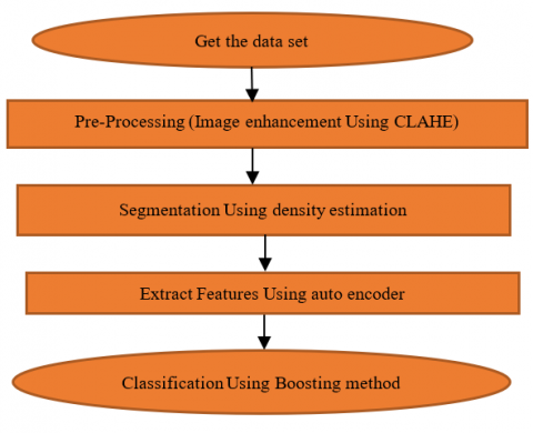
Figure 1. Proposed method
In the proposed method, after pre-processing the data, they are segmented by the density estimation method. In the next section, segmented image analysis by EEMD is discussed. Then, feature extraction is done by an auto encoder. Then the dimension reduction is done by the gray wolf algorithm. Eventually, images are classified into cancerous and non-cancerous categories using the boosting method. The flowchart of the proposed method is shown in Figure 1.
3.1 Pre-processing
One of the challenges of improving images is choosing the right method for the right improvement. Improvement in mammography images, especially dense breasts, is achieved by increasing contrast. The contrast between malignant tissue and breast tissue in a mammogram is below the threshold for human perception. Contrast Limited Adaptive Histogram Equalization (CLAHE) is one of the common techniques in which the contrast range is changed in such a way that the histogram is based on the cumulative distribution function of the desired shape. Therefore, CLAHE is used to improve image contrast and increase the contrast between masses and surrounding tissues [12].
3.2 Segmentation using density estimation
In this section, the segmentation based on density estimation is used with the help of the cumulus interactive thresholding method. This method allows for the separation of the dense parenchymal tissue part from the non-dense tissue part by manually adjusting the intensity threshold in mammography images. Then the density percentage (PD) is automatically calculated with the help of calculating the relative amount of dense tissue in the entire breast area. This method [13] proposed an interactive thresholding technique that selected gray-level thresholds from which the breast and dense tissue regions in the breast were identified. Then it calculates the density ratio of the radiograph from the histogram of the image [14-17].
3.3 Decomposition using EEMD
EMD method is a widely used algorithm for analyzing non-linear and non-stationary signals. This method is based on analyzing the signal into its constituent (Intrinsic Mode Functions) IMFs, the feature of IMFs is that each one has a significant instantaneous frequency. The necessary conditions for a signal to be selected as IMF (with significant instantaneous frequency) are as follows:
1-During the entire function data, the number of extremums and the number of zero crossings should be equal or their number should differ by at most one.
2-At any point, the average of the upper and lower layers should be zero. Normally, real signals do not have IMF conditions, and they must be converted to intrinsic mode functions, which are IMFs, using the Sifting Process algorithm.
The steps of the Sifting Process for the x(t) signal are as follows:
1-Determining all the relative extremes of the x(t) signal (maximums and minimums).
2-Obtain upper and lower cover using interpolation.
3-Calculation of the average of the top cover and the bottom cover.
4-The average difference between the high and low pass from the original signal.
5-Check if the resulting signal has the necessary conditions to be IMF or not. If so, it will be introduced as IMF, and if not, we will return to step 1 and go through the steps of the algorithm again. After calculating the first IMF, this function is subtracted from the initial signal and the remaining value is calculated. To extract the IMF of higher stages, the Sifting Process algorithm continues for the remainder of the previous stage. We continue this process until the remaining value has at least two extremes. After calculating all the IMFs, we can reach the initial signal by summing all of them with each other and the final remainder. Hilbert-Huang transformation is used to display IMFs in time-frequency space [15]. In the Hilbert-Huang transformation, the Hilbert transform is applied to the IMFs obtained from EMD. Hilbert transform of arbitrary signal c(t) is as follows:
$H(c(t))=\frac{1}{\pi} P V \int_{-\infty}^{+\infty} \frac{c(\tau)}{t-\tau} d r$ (1)
In relation 1, PV is the fundamental value of the Cauchy integral; in fact, it is the Hilbert transform of the convalescent signal c(t) concerning the function 1/t, which indicates the emphasis of the Hilbert transform on the local characteristics of the signal, including the amplitude and instantaneous frequency. Inspired by these advantages, the aim of this work is to employ EEMD to choose relevant IMFs for image classification.
3.4 Extract features using auto encoder
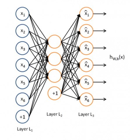
For the problems that arise in machine learning, we always need features that distinguish the inputs from each other to classify and recognize different data. The set of techniques that lead to learning these features is called feature extraction. Why do we need feature extraction? In machine learning, depending on the type of problem, the input can be very diverse. The input data often has a lot of redundancy, meaning that we do not need all the data values to solve the problem, and only a part of it is usable for us. On the other hand, due to the limitation in processing power in terms of memory and required time, we must extract a part of the inputs that are usable for us by performing transformations. Autoencoders are simple learning networks that are implemented to convert the input to output without the slightest change. At the same time, autoencoders play an important role in machine learning. For the first time, these concepts were proposed in 1980 by Hinton and the PDP research group. Along with Hebb's learning rules, autoencoders form one of the main paradigms of unsupervised learning. Autoencoders were again noticed in the first decade of the 20th century in deep architecture in the form of a bounded Boltzmann machine. Autoencoders are categorized under unsupervised learning. In this category of problems, there are no labels to describe the data (unlike supervised learning in which we use labels to describe the data). An autoencoder is a neural network that receives a set of unlabeled data and encodes them. It tries to re-represent the inputs in the output in such a way that they have the least possible difference from the input value. The image below shows an autoclave network. As you can see in Figure 2, the network is trained in such a way that the weights produced in the layers make the output have the minimum possible difference from the input, and in the most ideal case, they are equal.
The structure of the autoencoder is divided into two parts, encoding, and decoding. In the encoding section, the input data is mapped to the feature space, and in the decoding section, it is converted back to its original state from the feature space. The main part of an autoencoder is the middle hidden layer, which is used as an extracted feature for classification.
Feature extraction is a process used in machine learning to identify and select the most relevant features in a dataset, which can lead to several benefits. Firstly, it can improve the accuracy of a model's predictions by focusing on the most important features. Secondly, it can reduce the computational complexity of the model, making it faster and more efficient. Thirdly, it can improve the interpretability of the results by identifying the key features used in making the predictions. Fourthly, it can improve the generalization of the model, making it more effective at predicting new data. Finally, feature extraction can also improve the scalability of the model by reducing the dimensionality of the data, making it easier to scale up the model to handle larger datasets [16].
Figure 2. Feature extraction by auto coder [17]
3.5 Classification using boosting method
This concept is used to generate multiple models (for prediction or classification). Boosting algorithm was first used by Schapiro in 1990 so he proved that a weak classifier can become a strong classifier when it is placed in the format, probably approximately correct (PAC). Ad boost is one of the most famous algorithms. This family is considered to be one of the top 10 data mining algorithms. In this method, skewness is reduced along with variance, and margins are increased like support vector machines. This algorithm uses the entire data set to train each classifier, but after each training, it focuses more on hard data to classify correctly. This iterative method adaptively changes the distribution of the training data by focusing more on examples that have not been correctly classified before. At first, all the records get the same weight and the weights will increase in each iteration. The weight of misclassified samples will be increased, while the weight of those samples that are correctly classified will be decreased. Then, another weight is assigned separately to each classifier according to its overall accuracy, which is used later in the testing phase. Accurate classifiers will have a higher confidence factor. Finally, when presenting a new example, each classifier will propose a weight and the class label will be selected by a majority vote [18, 19]. Therefore, in the proposed method, this classifier is used to classify images into cancerous and non-cancerous categories.
In this section, the proposed method is tested on the data set. The proposed dataset includes 55,890 training samples, 14% of which are positive and 86% negative [20]. The dataset includes negative (non-cancerous) images from the DDSM dataset and positive (cancerous) images from the CBIS-DDSM dataset. The size of the images are all 299x299. Images are classified with two labels, First: label normal - 0 for negative (normal) and Socond 1 for positive (cancerous).So, there are two types of conditions 0 and 1. All the tests were done in MATLAB 2021 software with 16GB RAM and Windows 10.
4.1 Preprocessing and segmentation
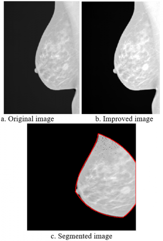
Figure 3. Image enhancement and segmentation
According to Figure 3 which shows 3 stages of segmentation in this research, in parts A and B, the uniformity of the histogram causes the contrast of the image to increase compared to its initial state, which means improving the quality of the image and increasing the accuracy of subsequent processing. Although this method can increase the contrast of the image, the resulting image usually has abnormal improvement and intensity saturation. However, it is powerful in defining the boundaries and edges between different objects. In addition, image B has more clarity and brightness and is more suitable for segmentation. So, image B was selected for this step. Now in part C, the boundaries of the image are well separated and the region of interest (ROI) is separated by the segmentation algorithm based on density estimation.
4.2 The results of decomposition by EEMD
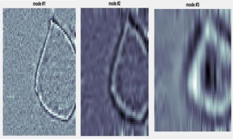
In this section, images are analyzed by the EEMD method into three levels as shown in Figure 4. This method is used to analyze non-linear and non-stationary image signals by separating them into components at different resolutions.
Figure 4. Image decomposition by EEMD
As can be seen in Figure 4, the analysis is done by three intrinsic modes on the segmented image. This work makes the features extracted by Auto Encoder to be well differentiated in the next steps and increases the classification accuracy.
4.3 The results of feature extraction
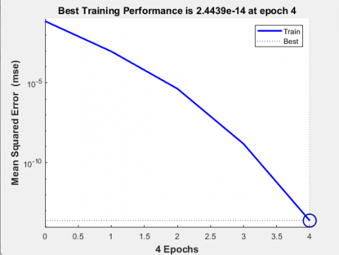
To extract features based on autoencoder, after training the data and repeating them, the MSE error rate has been significantly reduced in the best case Figure 5. The Figure indicates the performance at 4 Epochs.
Figure 5. MSE error rate of features by the autoencoder
As can be seen in Figure 5, the error rate by the proposed method decreases over time and reaches the optimal value, i.e., close to zero.
A neural network with a hidden layer has been used to encode this set. The hidden layer is made of 100 neurons. Each cell shows what features each of the hidden layer neurons are sensitive to and which feature is activated upon seeing. In its first layer, the autoencoder behaves like an edge detector and shows sensitivity to the edges in the image. It should be said that an autoencoder whose number of neurons in the hidden layer is less than the number of inputs is used to reduce the dimension.
4.4 Comparison with other methods
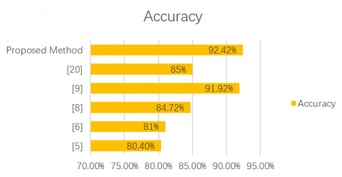
In this section, the proposed method has been compared and evaluated with other 6 selected methods, as shown in Figure 6 and Table 1. The range of difference from more accurate method (92.42%) to less (80.40%) is about 12.02%. This paper proposed method reach 92.42% of accuracy by developing EEMD method by utilizing feature extraction. These 6 methods were selected because they showed appopriate level of accuracy (more than 80%) and a comparison would become more valuable between these.
Figure 6. Qualitative comparison of the accuracy of the proposed method with other methods
Table 1. Accuracy of proposed method with other method
|
Accuracy |
|
|
[5] |
80/40% |
|
[6] |
81% |
|
[8] |
84/72% |
|
[9] |
91/92% |
|
[21] |
85% |
|
Proposed Method |
92/42% |
Although CNN was used in the method [9], the accuracy of the proposed method was obtained with a slightly better value. Reference method back-propagation neural networks and texture feature descriptors [8] has an accuracy of 84.72%. Next, histopathological image classification method [21] also has an accuracy of 85% which is close to back-propagation neural networks [8] result, and digital image processing algorithm [5] and [6] are in the next categories, respectively. As mentioned, in the proposed method, the single-layer auto encoder works like an edge detector. In the image above, the representation of the extracted features for the first layer shows the same point and has increased the accuracy. So, the results indicated that the EEMD with autoencoder-based methods and proposed feature extraction method vividly improve the accuracy of the classification in the mammography images.
Table 2. The quantitative criteria of the proposed method
|
Proposed Method |
Accuracy |
Sensitivity |
Specificity |
|
Bosting |
92.42 |
93.01 |
91.50 |
Now, in Table 2, the quantitative criteria of the proposed method for classification of the dataset of mammography images are shown. The result shows the Accuracy of 92.42%, sensitivity of 93.01%, and specificity of 91.50%.
In this article, the method based on the classification of breast cancer is presented. This work was done with the help of segmentation and analysis by EEMD. In this article, autoencoder-based structural features of cancerous masses extracted from digital mammography images by image processing methods have been used to classify the data into benign and malignant categories. In this research, after pre-processing the images by CLAHE, areas suspected of having cancerous masses in the breast tissue were extracted using the Autoencoder-based method. The proposed method was compared and evaluated with other methods. The results show that the accuracy of the proposed method is 92.41, which is better than other methods. The results show that the application and use of the autoencoder-based method increase the accuracy of the boosting algorithm in the data classification process.
[1] Azevedo, V., Silva, C., Dutra, I. (2022). Quantum transfer learning for breast cancer detection. Quantum Machine Intelligence, 4(1): 5. https://doi.org/10.1007/s42484-022-00062-4
[2] Dewangan, K.K., Dewangan, D.K., Sahu, S.P., Janghel, R. (2022). Breast cancer diagnosis in an early stage using novel deep learning with hybrid optimization technique. Multimedia Tools and Applications, 81(10): 13935-13960. https://doi.org/10.1007/s11042-022-12385-2
[3] Rasool, A., Bunterngchit, C., Tiejian, L., Islam, M.R., Qu, Q., Jiang, Q. (2022). Improved machine learning-based predictive models for breast cancer diagnosis. International Journal of Environmental Research and Public Health, 19(6): 3211. https://doi.org/10.3390/ijerph19063211
[4] Lin, R.H., Kujabi, B.K., Chuang, C.L., Lin, C.S., Chiu, C.J. (2022). Application of deep learning to construct breast cancer diagnosis model. Applied Sciences, 12(4): 1957. https://doi.org/10.3390/app12041957
[5] Robertson, S., Azizpour, H., Smith, K., Hartman, J. (2018). Digital image analysis in breast pathology-from image processing techniques to artificial intelligence. Translational Research, 194: 19-35. https://doi.org/10.1016/j.trsl.2017.10.010
[6] Liu, X., Chen, K., Wu, T., Weidman, D., Lure, F., Li, J. (2018). Use of multimodality imaging and artificial intelligence for diagnosis and prognosis of early stages of Alzheimer's disease. Translational Research, 194: 56-67. https://doi.org/10.1016/j.trsl.2018.01.001
[7] Mohamed, B.A., Salem, N.M. (2018). Automatic classification of masses from digital mammograms. In 2018 35th National Radio Science Conference (NRSC), March 20-22, 2018. Cairo: IEEE, pp. 495-502. https://doi.org/10.1109/NRSC.2018.8354408
[8] Pérez, M., Benalcázar, M.E., Tusa, E., Rivas, W., Conci, A. (2017). Mammogram classification using back-propagation neural networks and texture feature descriptors. In 2017 IEEE Second Ecuador Technical Chapters Meeting (ETCM), October 16-20, 2017. Salinas: IEEE, pp. 1-6. https://doi.org/10.1109/ETCM.2017.8247515
[9] Castro-Tapia, S., Castañeda-Miranda, C.L., Olvera-Olvera, C.A., Guerrero-Osuna, H.A., Ortiz-Rodriguez, J.M., Martínez-Blanco, M., Díaz-Florez, G., Mendiola-Santibañez, J.D., Solís-Sánchez, L.O. (2021). Classification of breast cancer in mammograms with deep learning adding a fifth class. Applied Sciences, 11(23): 11398. https://doi.org/10.3390/app112311398
[10] Vijayarajeswari, R., Parthasarathy, P., Vivekanandan, S., Basha, A.A. (2019). Classification of mammogram for early detection of breast cancer using SVM classifier and Hough transform. Measurement, 146: 800-805. https://doi.org/10.1016/j.measurement.2019.05.083
[11] Arooj, S., Zubair, M., Khan, M.F., Alissa, K., Khan, M.A., Mosavi, A. (2022). Breast cancer detection and classification empowered with transfer learning. Frontiers in Public Health, 10: 924432. https://doi.org/10.3389%2Ffpubh.2022.924432
[12] Vidhya, G.R., Ramesh, H. (2017). Effectiveness of contrast limited adaptive histogram equalization technique on multispectral satellite imagery. In Proceedings of the International Conference on Video and Image Processing, December 27-29, 2017. Singapore: Association for Computing Machinery, pp. 234-239. https://doi.org/10.1145/3177404.3177409
[13] Boyd, N.F., Martin, L.J., Bronskill, M., Yaffe, M.J., Duric, N., Minkin, S. (2010). Breast tissue composition and susceptibility to breast cancer. Journal of the National Cancer Institute, 102(16): 1224-1237. https://doi.org/10.1093/jnci/djq239
[14] Pertuz, S., Sassi, A., Holli-Helenius, K., Kämäräinen, J., Rinta-Kiikka, I., Lääperi, A.L., Arponen, O. (2019). Clinical evaluation of a fully-automated parenchymal analysis software for breast cancer risk assessment: A pilot study in a Finnish sample. European journal of radiology, 121: 108710. https://doi.org/10.1016/j.ejrad.2019.108710
[15] Bhardwaj, N., Nara, S., Malik, S., Singh, G. (2016). Analysis of ECG signal denoising algorithms in DWT and EEMD domains. International Journal of Signal Processing Systems, 4(5): 442-445. https://doi.org/10.18178/ijsps.4.5.442-445
[16] Becker, D.S., Larsen, K.R. (2021) Automated Machine Learning for Business. Oxford University Press.
[17] Yang, X.J., Wu, L., Zhao, K., et al. (2020). Evaluation of human epidermal growth factor receptor 2 status of breast cancer using preoperative multidetector computed tomography with deep learning and handcrafted radiomics features. Chinese Journal of Cancer Research, 32(2): 175-185. https://doi.org/10.21147%2Fj.issn.1000-9604.2020.02.05
[18] Wu, Y. (2021). Application of improved boosting algorithm for art image classification, Hindawi Scientific Programming, Article ID: 3480414. https://doi.org/10.1155/2021/34804144.
[19] Zhong, K., Wang, Y., Pei, J., Tang, S., Han, Z. (2021). Super efficiency SBM-DEA and neural network for performance evaluation. Information Processing & Management, 58(6): 102728. https://doi.org/10.1016/j.ipm.2021.102728
[20] Lee, R.S., Gimenez, F., Hoogi, A., Rubin, D. (2016). Curated breast imaging subset of DDSM. The Cancer Imaging Archive.
[21] Spanhol, F.A., Oliveira, L.S., Petitjean, C., Heutte, L. (2015). A dataset for breast cancer histopathological image classification. IEEE Transactions on Biomedical Engineering, 63(7): 1455-1462. https://doi.org/10.1109/TBME.2015.2496264