Lügen Ünal* | Ahmet Güngör Pakfiliz
© 2022 IIETA. This article is published by IIETA and is licensed under the CC BY 4.0 license (http://creativecommons.org/licenses/by/4.0/).
OPEN ACCESS
Low probability of intercept (LPI) radar systems is designed "to see and not to be seen." Low peak power, low sidelobe antenna pattern, wide bandwidth, and spread spectrum waveform are their typical characteristics to prevent detection by noncooperative electronic warfare receivers. As a result, in terms of Electronic Warfare systems, the detection of an unknown LPI radar has great importance and requires special techniques. While a few studies have been done on this subject, many open points still need to be managed. This paper presents an LPI radar signal detection algorithm based on autocorrelation and time-frequency image-based moments. Detection does not require any prior information on radar signals. Detection performance for different types of LPI radar signal waveform is studied. The results showed that detection is possible under low SNR.
LPI radar, spread spectrum, signal detection, time-frequency analysis, image moment, connected component labeling
As the name implies, the Low Probability of Intercept (LPI) radar system's main objective is to escape detection by intercept receivers while providing its mission. For various reasons, radar designers are now working on waveforms that perform the same radar functions but are more difficult to intercept. (One reason is the threat of attack Anti Radiation Missiles) [1]. In addition, Radar users are concerned about Electronic Warfare (EW) technology because transmitted signals will leak radar operating parameters to enemy ES/ELINT systems. To attack this issue, radar designers concentrate on the advanced and revolutionary RF stealth concept, LPI [2].
LPI radar can find an extensive place in a tactical environment. Radar altimeters, LPI landing systems, surveillance, fire control radars, and anti-ship capable missiles are some of the systems that use LPI technology [3].
Low antenna side lobes, aperiodic scan pattern, power management, and low transmit power are among the LPI radar properties. LPI radars, when compared with conventional radars, transmit weak signals over a wide frequency band. This property makes it difficult for the intercept receiver to detect the signals above its threshold. Thus, the LPI radar operation creates a scenario for the intercept receiver that looks like a noisy signal receiving all the time [2]. The radiated energy spread over a wide bandwidth is named a spread spectrum (SS) waveform.
SS also called pulse compression in radar systems, is used for several reasons [4]. The simultaneous requirements of extensive maximum range, high range resolution, and high Doppler resolution have led radar and sonar designers to utilize pulse modulation techniques for providing large time-bandwidth product waveforms known as pulse compression waveforms [5]. SS waveform is one of the essential properties of an LPI radar system. It was a natural result of the Second World War. SS grew in communication and radar technology simultaneously. Some of the SS techniques employed to achieve wide-band signals are pure noise, direct sequence (DS), frequency modulation, frequency hopping (FH), and time hopping (TH). DS systems employ pseudorandom sequences and phase-shift keying (PSK) onto the carrier for spreading. TH to spread the carrier is achieved by randomly spacing a narrow transmitted signal. In communication, frequency and time hopping were recognized anti-jamming concepts during the early 1940s. The DS concept followed the FH and TH concepts for several years. SS, for jamming avoidance and resolution, was a concept familiar to radar engineers by the war's end [6].
SS (pulse compression) LPI radar waveform modulation techniques are Linear Frequency Modulation (LFM), Nonlinear Frequency Modulation (NLFM), Frequency Modulation Continuous Wave (FMCW), Phase Shift Keying (PSK), Frequency Shift Keying (FSK) or FH, hybrid FSK/PSK techniques, and noise technique [7, 8]. Though DS Spread Spectrum (DSSS) technique originally grew in communication systems, the DSSS waveform for radar applications is represented as an LPI technique used for various reasons, such as to combine communication and radar functions in the same waveform or Multiple Input Multiple Output (MIMO) radar technique in the studies [9-12].
For LPI radar systems, PSK modulation is managed by using binary or polyphase codes. The Barker codes are the prevalently used binary code. On the other hand, polyphase Barker, Frank, P1, P2, P3, P4 are polyphase codes used in PSK modulation of LPI radar waveforms. Polyphase is the most frequently used code because of easy digital implementation, versatility, high range resolution, and Doppler tolerance [13]. There are also T1, T2, T3, and T4 types codes called polytime codes used for PSK modulation.
The LPI radar CW waveform is more popular than PW [14]. The advantage of CW usage is that CW radar has low peak power compared to high peak power for pulsed radar for the same detection performance.
As for the subject of non-cooperative LPI radar transmission detection, EW receivers such as RWR (Radar Warning Receiver), ES/ESM (Electronic Support/Electronic Support Measurement), or ELINT (Electronic Intelligence) receivers are in question. Because of LPI radars' ever-increasing and widespread usage in tactical environments, LPI radar waveform detection and recognition is a vital problem in EW systems. EW system tries to detect a blindly intercepted enemy radar signal and analyze its capabilities before generating a jamming signal [15]. High-sensitivity digital receivers with wide bandwidth are used for LPI radar signal interception and analysis [16]. Spectrum sensing techniques for Cognitive Radio and Radar systems are categorized as matched-filter, energy-detection and feature-detection methods [17]. Feature detection refers to extracting features from the received signal and performing detection based on the extracted features. Typical features are stated as correlation-based features. This grouping methodology can be taken into account for radar EW receivers. The EW detection techniques seen in literature named autocorrelation detection for DSSS signals [18], as with cross-correlation based detection [19] and Time-Frequency (TF) domain detection techniques given in [3] can take place in the feature detection techniques. The matched filter requires knowledge of the received signal, which is unsuitable for non-cooperative EW receivers [20]. On the other hand, energy detection is a simple method. It does not require prior knowledge of the signal. It computes the signal's energy and compares it to a threshold to decide signal presence. This study uses a combination of correlation detection and TF detection techniques.
TF analysis techniques are Wigner-Ville distribution (WVD), Choi-Williams distribution (CWD), Quadrature Mirror Filter Bank (QFMB), Wavelet transform, Short Time Fourier Transform (STFT), and S Transform. Cyclostationary Spectral (CS) analysis is a bi-frequency analysis technique that is used for LPI radar signal detection and parameter extraction [3, 21].
A method based on modified Wigner Hough Transform (WHT) is applied to detect Frank, P1, P2, P3, P4, and LFM types LPI radar signals and detection performance compared to Generalized (WHT) [13]. QMFB analysis is used for parameter extraction in P1, P2, P3, and P4 type polyphase signals [22]. The extracted parameters from the TF image are carrier frequency, number of phases, and cycle per phase. Up to -4 dB SNR, successful results are presented. Parallel filter arrays and higher-order statistics are used to detect FMCW, Frank, Costas, and P4-coded LPI radar waveforms [23]. FMCW and P4 signal detection performance based on QMFB is studied [24]. An algorithm is proposed to detect and identify the parameters of the LPI signals like frequency, pulse width, pulse repetition interval (PRI), and modulations using STFT [25]. Cyclo-stationary (CS) method is used to estimate the parameters of polytime-coded LPI signals [21]. The Time-frequency plane is obtained from the modified S transform extracts P1, P2, P3, and P4 type polyphase radar signal parameters [26]. Up to -4 dB SNR, parameter extraction can be managed except for the carrier frequency. A statistical detector of a hypothesis test is given [27]. The test function variable is a feature vector based on the intercepted signal's first and second moments of WVD. One of the features is the orientation of the principal axes. The Radial Basis Function Neural network estimates the probability density function of the feature vector. An exemplary detection performance at low SNR is represented for the FMCW signal. In this study orientation angle of WVD is also used as a detection parameter, but WVD is handled as an image, and the orientation angle is determined by image moments.
Detection handles like a time series problem, and Recurrent Neural Network (RNN) based denoising autoencoder is proposed to detect LPI radar signal [28]. Twenty-three types of LPI signals are analyzed. Detection occurs up to -5 dB SNR. First [29], the signal intercepted by the electronic warfare receiver is subjected to wavelet noise reduction preprocessing, and its autocorrelation is calculated. After autocorrelation, the signal is converted into a Visibility Graphs complex network. Then, using the network's average degree, the detection threshold is calculated by setting the false alarm probability value of the pure Additive White Gaussian Noise (AWGN) noise signal, and the real signal is detected.
LPI radar signal detection based on correlation techniques uses the periodic structure of radar waveforms. LPI radar waveforms are modulated by a periodic function [3]. Additionally, the autocorrelation sequence of a periodic signal is also periodic. This property helps the detection of LPI radar signals by ES receivers. An LPI airborne radar of LFM waveform detection and location process by two passive receivers problem is considered [19]. The digital correlation method takes advantage of the signal being periodic but noise random. The study represented the detection of weak periodic signals by digital correlation. The autocorrelation sequence will reach every interval of the signal's period. Therefore, signal periodicity can be estimated. Mixing product (correlation) of intercepted signals by different passive receivers also estimates different times of arrival.
As for the automatic classification task of the EW receiver, machine learning algorithms have become apparent in recent studies [7, 14, 29-32]. In these studies, the classification is based on features obtained from the TF distribution of the detected signal. These features are input to the classification method.
The intercepted signal WVD and CWD computation performed first, then the combination of the 'single shot multi-box detector (SSD)' and 'you only look once version 3' (YOLOv3) is used for the classification of LPI radar signals [14]. Support Vector Machine (SVM) and k-Nearest Neighbor (kNN) algorithms are used to classify the extracted features [29]. New features based on Wigner and Choi-Williams TF distributions are proposed [30]. These features allow a parallel classifier structure based on a multilayer perception network to classify LFM, Costas, Frank, BPSK, P1, P2, P3, and P4 waveforms. The received signals are transformed to obtain the time-frequency matrix by CWD [31]. Then waveform recognition is performed based on dictionary learning. LFM, NLFM, Costas, Frank, P1, P2, P3, and P4 coded waveform classified. STFT is used to construct entry images. Improved GoogLeNet and ALexNet architecture as Convolutional Neural Networks (CNN) is utilized to detect and classify LPI radar signals [7]. The features are extracted from the Choi-Williams time-frequency distribution (CWD) image of the received data, and Elman Neural Network is selected as the classifier [32].
Other classification techniques do not include machine learning algorithms or TF distribution. The signal is estimated using WVD at the first stage [2]. Features required for the automatic classification are derived using Radon Ambiguity Transform and Radon-WVD and proposed novel features based on the fractional Fourier Transform. The detection performances of LPI Radar signals with Wigner Ville Distributions are examined by treating each distribution as an image [33]. The classification can be performed with an image processing algorithm that an eigen image approach over Wigner-Ville Distributions. Results were represented for P1 coded waveforms. Autocorrelation function (ACF) based classification is given in the study of [34]. The ACFs of analytic radar signals are calculated to magnify the discrimination of signals of different categories. A simple de-noising approach is introduced to purify the ACFs. Four features are extracted from the purified ACF. A Directed Graphical Model (DGM) is used to represent the joint probability distribution of the four features along with the category and to classify unknown radar signals.
In this study, we focus on a detection technique that is a mixture of ACF based detection and WVD image feature-based detection. The detection performance is shown on FMCW and different PSK LPI radar waveforms. Simulation results are compared with the energy detection technique and superiority of the proposed method are demonstrated. The contribution of our study is to provide a robust LPI Radar signal detection method. Despite most of the detection in literature being based on time-frequency analysis detection, this article analyzed a wide variety of waveforms and studied autocorrelation-based detection. Wigner-Ville distribution-based solution was conducted in the receiver structure, and a new noise reduction method was performed on the WVD image to support the detection decision.
The rest of the paper is organized as follows: Sections 2 and 3 introduce the transmitted and received signal model, respectively, and Section 4 introduces the existing detection methods. Section 5 presents the proposed method and simulation results of the method, and a conclusion is presented in section 6.
In this study, PSK-modulated CW signals and FMCW signals are analyzed. In the analysis, signals are used in the analytic form. By forming the analytic signal, the negative frequency components of a real signal may be eliminated from the signal representation without losing information. This elimination provides sampling below the Nyquist rate and avoids interference terms by the interaction of positive and negative components in quadratic TFDs [35], the analytic form of the transmitted radar waveform expressed as
$s(t)=A e^{j\left(2 \pi f_c t+\emptyset_k\right)}$ (1)
The in phase (I) and quadrature (Q) component of s(t) is defined as
$I=A \cos \left(2 \pi f_c t+\emptyset_k\right)$ (2)
$Q=A \sin \left(2 \pi f_c t+\emptyset_k\right)$ (3)
where, A is the amplitude, $f_c$ is the carrier frequency of the transmit signal and $\emptyset_k$ is the phase of the signal. For FMCW signal, phase is constant and carrier frequency changes in a symmetric triangular waveform such as:
for the up-ramp of the signal: $f_c-\frac{\Delta F}{2}+\frac{\Delta F}{t_m} t$ (4)
for the down-ramp of the signal: $f_c+\frac{\Delta F}{2}+\frac{\Delta F}{t_m} t$ (5)
where, $\Delta F$ is the transmit modulation bandwidth and $t_m$ is the modulation period.
For PSK signals, the carrier frequency is constant. Instead of frequency, phase values are changed by specific codes such as binary phase codes, polyphase codes, or polytime codes. PSK modulated signal's phase changes after every subcode period $t_b$. Consequently, the code period T and code rate $C_R$ are defined as:
$T=N_c t_b$ (6)
$C_R=\frac{1}{N_c t_b}$ (7)
where, $N_c$ represents the number of phase codes and represents the code length as well. The duration of the transmitted signal is$P \times T$, where P is the number of periods.
If cpp is the number of cycles of the carrier frequency per subcode, the bandwidth of the transmitted signal is
$B=\frac{f_c}{c p p}=\frac{1}{t_b} \mathrm{~Hz}$ (8)
For polyphase-encoded waveforms, using $c p p=1$ results in the maximum bandwidth achievable with any carrier frequency. The shorter the duration of the subcode period, the greater the bandwidth. On the other hand, for polytime codes $t_b$ is not constant. Polytime code sequences use fixed phase states with varying periods at each phase state. Polytime coded waveforms bandwidth is measured due to the shortest phase change duration. Polytime coding has the advantage that arbitrary time bandwidth waveforms can be generated with only a few phase states. An increase in code lengths of PSK waveform does not affect bandwidth but increases the processing gain. The processing gain is equal to the compression ratio of the signal. For both the frequency modulation and phase modulation LPI radar, the transmitted CW signal is coded with a reference signal to spread the transmitted energy in frequency [3]. The codes with zero sidelobes in periodic ACF (PACF) are called perfect codes. The low sidelobe levels of the ACF and PACF help quantify the LPI waveform's ability to detect targets without interfering with sidelobe targets. High sidelobes might be caused nearby targets to hide in a sidelobe [36]. Frank, P1, P3, and P4 codes have perfect PACF [3, 37]. Polyphase is the most frequently used code because of easy digital implementation, versatility, high range resolution, and Doppler tolerance [13]. The specific codes used in LPI radar waveform PSK modulation is given below.
2.1 Binary barker codes
A binary Barker sequence is a finite length, discrete time sequence $A=\left\{a_0, a_1, \ldots, a_n \right\}$ of $+1^{\prime}$ s and $-1^{\prime}$ s of length $n \geq 2$, such that the aperiodic autocorrelation coefficients (or sidelobes):
$r_k=\sum_{j=1}^{n-k} a_j a_{j+k}$ (9)
Satisfies $\left|r_k\right| \leq 1$ for $k \neq 0$ and similarly $r_{-k}=r_k$. The Binary Barker sequences correspond the phase values of $0^{\circ}$ or $180^{\circ}$ used for BPSK modulation.
Binary Barker codes are only known for lengths $N_c=2,3,4,5,7,11$ and 13 given in Table 1 [38].
Table 1. Binary codes
|
Code length ( $N_c$) |
Code elements |
|
2 |
-+,++ |
|
3 |
++- |
|
4 |
++-+ |
|
4 |
+++- |
|
5 |
+++-+ |
|
7 |
+++--+- |
|
11 |
+++---+--+- |
|
13 |
+++++--++-+-+ |
2.2 Polyphase barker codes
Polyphase code sequences correspond to more than two phase values. Their alphabet size $N_c>2$. The idea of increasing the size of the alphabet for constructing Barker sequences was completed in 1965 by Golomb and Scholz. Golomb and Scholz introduced the concept of Generalized Barker codes, defined as a multiphase sequence [39]. Allowing any phase values (nonbinary) can lead to lower sidelobes. However, the outermost sidelobe is always 1 [37]. Consider the generalized Barker sequences $\left\{a_j\right\}$ of finite length n where the terms $a_j$ are allowed complex numbers of absolute value of 1 where the correlation is now Hermetian dot product.
$r_k=\sum_{j=1}^{n-k} a_j a_{j+k}^*$ (10)
where, $a^*$ represents the complex conjugate of a . If all the sidelobes of the ACF of any polyphase sequence are bounded by
$|r(k)| \leq 1$ for $k \neq 0$ (11)
Then the sequence is called generalized Barker sequence or polyphase Barker sequence. The binary Barker sequences can be regarded as a special case of polyphase Barker sequences. If the sequence elements are taken from an alphabet of size M , consisting of the $M^{t h}$ roots of unity,
$a_m=\exp \left\{2 \pi i \cdot \frac{m}{M}\right\}=: \exp \left(i \emptyset_m\right) \ 0 \leq m \leq M-1$ (12)
The sequence is alternatively named an M-phase Barker sequence [40]. Polyphase Barker signal is difficult to intercept and correctly classify using the ES system [2]. In many applications, the phases are restricted to values that are the kth roots of unity (e.g, $k^{}= 2$ gives the original Barker codes or $k^{}= 6$ for six phase/sextic Barker codes). As for polyphase Barker codes, systematic methods to construct polyphase Barker sequences have not been found yet. Searches for generalized Barker sequences with no restriction on the values of the sequence phases have been carried out using numerical optimization [37].
2.3 Frank code
Frank code derived from the phase history of a linearly frequency stepped pulse, using M frequency steps and M samples per frequency. The number of code elements is equal to $M^2$. The elements of the original Frank code $a_{(n-1) M+k}=\exp \left(j \emptyset_{n, k}\right)$, for $1 \leq n \leq M$ and $1 \leq k \leq M$. The phase values are expressed as:
$\emptyset_{n, k}=\frac{2 \pi}{M} (n-1)(k-1), \quad n=1,2, \ldots, M$ and $k=1,2, \ldots, M$ (13)
where, n is the number of the sample in a given frequency and k is the number of the frequency.
2.4 P1, P2, P3 and P4 code
P1 and P2 signals are derived from step approximation to a linear frequency modulated waveform. In these codes using M frequency steps and M samples per frequency are produced. P3 and P4 signals are derived from linear frequency modulated waveform. Phase equations of P-codes given in Table 2.
Table 2. P1-P2-P3-P4 Codes and phase equation
|
Code type |
Phase |
|
P1 |
$$\emptyset_{i, j}=\frac{-\Pi}{M}[M-(2 j-1)][(j-1) M+(i-1)],$$where $i=1,2, \ldots, M$ and $j=1,2, \ldots, M$ |
|
P2 |
$$\emptyset_{i, j}=\frac{-\pi}{2 M}[2 i-1-M][2 j-1-M],$$where $i=1,2, \ldots, M$ and $j=1,2, \ldots, M$ |
|
P3 |
$\emptyset_i=\frac{\pi}{N_c}(i-1)^2, \quad i=1,2, \ldots, N_c$ |
|
P4 |
$\emptyset_i=\frac{\pi(i-1)^2}{N_c}-\pi(i-1), \quad i=1,2, \ldots, N_c$ |
2.5 Polytime codes
$T 1(n)$ and $T 2(n)$ types of polytime code can be generated from the stepped frequency model, $T 3(n)$ and $T 4(n)$ types are approximations to a linear frequency modulation.
Phase versus time relation of $T 1(n)$ and $T 3(n)$ code $\emptyset_{T 1}(t), \emptyset_{T 3}(t)$, are expressed as follows, respectively,
$\emptyset_{T 1}(t)=mod \left\{\frac{2 \pi}{n} I N T\left[(k t-j T) \frac{j n}{T}\right], 2 \pi\right\}$ (14)
$\emptyset_{T 3}(t)=mod \left\{\frac{2 \pi}{n} I N T\left[\frac{n \Delta F t^2}{2 t_m}\right], 2 \pi\right\}$ (15)
In Eq. (14), $j=0,1,2, \ldots, k-1$ is the segment number in the stepped frequency waveform, k is the number of the segments in the T1 code sequence, t is the time, T is the overall code duration, n is the number of phase states in the code sequence. In Eq. (15), $t_m$ is the modulation period, and $\Delta F$ is modulation bandwidth. As more phase states are added to the polytime sequence, the agreement in time sidelobe behavior improves [3].
An example of LPI radar signal which is PSK modulated by Frank code where $N_c=64, \mathrm{f}_{\mathrm{c}}=1 \mathrm{kHz}$, cpp=1, $\mathrm{SNR}=-6 \mathrm{~dB}$ shown in Figure 1.
Figure 1. Frank coded waveform, SNR = -6 dB
The signal at the output of the receiver filter is expressed as
$\mathrm{x}(t)=\mathrm{s}(t)+\mathrm{n}(\mathrm{t})$ (16)
where, $s(t)$ is transmitted noiseless radar signal and $n(t)$ is complex zero mean Additive White Gaussian Noise (AWGN) with variance $\sigma^2$. Power spectral density of White Noise is $\frac{N_0}{2}$. where, $N_0$ is watts per Hertz and it may be expressed as $N_0=k T_e$ where k is the Boltzmann's constant and $k T_e$ is the equivalent noise temperature of the receiver [41]. For Gaussian noise, the filtered White Noise, with a filter bandwidth W , can be represented by a sequence of independent, zero-mean, Gaussian random variables with variance $\sigma^2=\mathrm{N}_0 W$. The variance of the samples and the rate at which they are taken are related by $\sigma^2=\mathrm{N}_0 \mathrm{f}_{\mathrm{s}} / 2$ ( $\mathrm{f}_{\mathrm{s}}$ is sampling rate) [42].
4.1 Autocorrelation based signal detection
This section presents spread spectrum DSSS and radar signals detection methods. DSSS signal detection by autocorrelation is subcategorized as single-channel autocorrelation, dual-channel autocorrelation, and compounded autocorrelation [18]. Detection results from the exploitation of cyclostationary of DSSS signals and similar communication transmissions by correlating received signals. Detection is performed by analyzing correlation peaks. The fluctuation of correlation estimators method is presented to detect DSSS signals [43]. This method is the same as compounded autocorrelation mentioned in the study of [18]. The idea behind this technique is that a DSSS signal's autocorrelation is like a noise's autocorrelation. On the other hand, the fluctuations of estimators are different. The detection is based on the peaks of fluctuations.
The autocorrelation sequence of a periodic signal is periodic too. This property is used for the detection and parameter estimation of LPI radar signals [19]. The autocorrelation function is also used to filter out the noise. In [44], for LPI radar signal detection, autocorrelation processing of the signal is used to filter out the noise, and radar signal classification is performed based on features obtained from the autocorrelation function and directed graphical model.
Periodic heritage and noise reduction property of the ACF explained below:
When $x(t)$ is the observable signal at the receiver output is given in Eq. (16), the autocorrelation function of $x(t)$ is
$\begin{aligned} & R_{x x}(\tau)=E[x(t) x(t-\tau)] \\ & =E\{[s(t)+n(t)][s(t-\tau)+n(t-\tau)]\} \\ & =E[s(t) s(t-\tau)]+E[n(t) n(t-\tau)] \\ & +E[s(t) n(t-\tau)] \\ & +E[n(t) s(t-\tau)] \\ & =R_{s s}(\tau)+R_{n n}(\tau)+R_{s n}(\tau)+R_{n s}(\tau)\end{aligned}$ (17)
$R_{s n}(\tau)=R_{n s}(\tau)=0$ since the noise is not related to the s(t). Hence
$R_{x x}(\tau)=R_{s s}(\tau)+R_{n n}(\tau)$ (18)
For zero mean AWGN with wide bandwidth, the autocorrelation function $R_{n n}(\tau)$ mainly affects the nearby position $\tau=0$.
$R_{n n}(\tau)=\sigma^2 e^{-\alpha|\tau|}$ for $|\tau| \gg 1$ (19)
Hence $R_{x x}(\tau) \approx R_{s s}(\tau)$ [19, 34, 44].
4.2 Time frequency analysis based detection
Time-frequency $(t, f)$ methods can be grouped into amplitude (linear) "atomic" decompositions and "energy" quadratic (or bilinear) distributions. The linear class represents a signal as a linear combination of a family of elementary signals (called atoms) that are well localized in time and frequency. The linear class includes the short-time Fourier transform (STFT) and the wavelet transform (WT). The bilinear class includes quadratic TFDs (QTFDs) that distribute the energy of the signal between two variables, namely time and frequency (or time and scale). Wigner Ville Distribution (WVD) is a bilinear distribution. All other QTFDs are filtered versions of the WVD. Windowed versions of the WVD are the pseudo WVD (PWVD), and smoothed pseudo WVD used to improve TF representations [35]. The WVD of a signal $s(t)$ denoted by $W_z(t, f)$, is defined as:
$W_z(t, f)=\underset{\tau \rightarrow f}{\mathcal{F}}\left\{z\left(t+\frac{\tau}{2}\right) z^*\left(t-\frac{\tau}{2}\right)\right\}$ (20)
where, $z(t)$ is complex and defined as the analytic associate of $s(t)$. So, the WVD of signal $s(t)$ is given as:
$W_z(t, f)=\int_{-\infty}^{+\infty} z\left(t+\frac{\tau}{2}\right) z^*\left(t-\frac{\tau}{2}\right) e^{-j 2 \pi f \tau} d \tau$ (21)
WVD is also defined as the Fourier transform of the instantaneous autocorrelation function of a signal $z(t, f)$ [45]. The marginal integration of TFD of WVD over frequency and time gives instantaneous power and energy spectrum of the signal respectively that are given Eqns. (22) and (23).
$\int_{-\infty}^{+\infty} W_z(t, f) d f=|z(t)|^2$ (22)
$\int_{-\infty}^{+\infty} W_z(t, f) d f=|z(f)|^2$ (23)
The integration of the WVD over the entire $(t, f)$ plane yields the signal energy $E_z$.
$\int_{-\infty}^{+\infty} \int_{-\infty}^{+\infty} W_z(t, f) d t d f=E_z$ (24)
The discrete WVD expressed as:
$W(l, w)=2 \sum_{-\infty}^{+\infty} z(l+n) z^*(l-n) e^{-j 2 w n}$ (25)
Windowing the data results in the pseudo-WVD and is defined by:
$\begin{array}{r}W(l, w)=2 \sum_{n=-N+1}^{N+1} z(l+n) z^*(l-n) \ldots \\ \ldots w (n) w(-n) e^{-j 2 w n}\end{array}$ (26)
where, $w(n)$ is a length $2 N-1$ real window function with $w(0)=1$. The two drawbacks of WVD are negative values and cross terms. Because of its bilinear structure WVD has cross terms appear in the middle of every pair of signal components. WVD can have large negative values. Most TFDS used in practical applications can take negative values as they are not necessarily positive definite, so they do not represent and instantaneous energy spectral density at any arbitrary $(t, f)$ location [35]. One of the features that can be extracted from the Time-frequency distributions is joint time frequency moments. The two-dimensional moment of order $(p+q)$ of a time frequency distribution $T F D(t, f)$ is defined as:
$M_{p q}=\int_{-\infty}^{+\infty} \int_{-\infty}^{+\infty} t^p f^q T F D(t, f) d t d f$ (27)
The central moments of $T F D(t, f)$ is defined as:
$\mu_{p q}=\int_{-\infty}^{+\infty} \int_{-\infty}^{+\infty}(t-\bar{t})^p(f-\bar{f})^q T F D(t, f) d t d f$ (28)
where, $\bar{t}$ and $\bar{f}$ are defined as:
$\bar{t}=\frac{M_{10}}{M_{00}}, \quad \bar{f}=\frac{M_{01}}{M_{00}}$ (29)
4.3 Energy detector
The energy detector computes the energy in the received data and compares it to a threshold. The energy detector (ED) for an unknown deterministic signal $x[n]$ is expresses as
$T(x)=\sum_{n=0}^{N-1} x^2[n]>\gamma$ (30)
where, $x[n]$ is signal pluse noise under hypothesis H1, only noise signal under hypothesis H0. $T(x)$ is called the test statistics. ED decides H1 if $T(x)$ is greater than the threshold. Under H0, the received signal is chi-squared distributed which probability density function given as [28, 46].
$p(x)= \begin{cases}\frac{1}{2^{\frac{v}{2}-} \Gamma\left(\frac{v}{2}\right)} x^{\frac{v}{2}-1} \exp \left(-\frac{1}{2} x\right) & x>0 \\ 0 & x<0\end{cases}$ (31)
where, v is degree of freedom.
The threshold determined by a given probability of false alarm rate $\left(P_{F A}\right)$.
It is given that if the number of sampled signals (N) is large enough and the channel is nonfading [47], the chi-square distribution with N degrees of freedom can be considered as a normal distribution by using the central limit theorem, and $P_{F A}$ written as
$P_{F A}=Q\left(\frac{\gamma-M N \sigma^2}{\sigma^2 \sqrt{2 M N}}\right)$ (32)
where, $\sigma^2$ is the noise variance and M is antenna number.
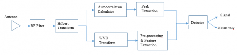
The proposed solution consists of cooperation of two modules as given Figure 2. First, the intercepted signal passes through an RF filter, and IF conversion occurs. Then to get analytic signal form Hilbert Transform (HT) is performed. The analytic signal's ACF and WVD are calculated after HT.
Figure 2. Block diagram of proposed solution
In the Autocorrelation Calculator block, autocorrelation is performed on the obtained signal, then an empirical threshold value set for denosing, and then search periodic peaks, which will occur if the signal has a periodic structure and does not occur if there is only a noise signal. At least two peaks are required to determine the radar signal. Also, one can determine the code period from the number of data points between periodic peaks.
While performing ACF and peak extraction simultaneously, PWVD transform occurs in the second block of the receiver. The signal decision is given according to the PWVD image orientation angle. The pre-processing stage requires binary image transformation of the PWVD of the intercepted signal.
Pre-processing steps are:
Connected-component labeling is a fundamental task common to virtually all image processing applications in two- and three-dimensional. For a binary image, represented as an array of d-dimensional pixels or image elements, connected component labeling assigns labels to the black image elements so that adjacent black image elements are assigned the same label. Here adjacent may mean 4-adjacent or 8-adjacent. Connected-component labeling can be characterized as a transformation of a binary input image, B, into a symbolic image, S, such that [48]
For an $N x N$-sized binary image, the pixel at the coordinate $(x, y)$, where $0 \leq x \leq N-1$ and $0 \leq y \leq N-1$ , in the image is denoted as $b(x, y)$. For pixel $b(x, y)$, the four pixels, the four pixels $b(x-1, y)$ , $b(x, y-1)$, $b(x+1, y)$ and $b(x, y+1)$ are called the 4-neighbors of the pixel; the 4-neighbors together with the four pixels $b(x-1, y-1)$, $b(x+1, y-1)$; $b(x-1, y+1)$; and $b(x+1, y+1)$ are called the 8-neighbors of the pixel [49].
In this study, CCL is used to denoise the WVD binary image of the received signal. 8-connected labeling is used. If the received signal is an LPI radar signal, the WVD image would have a specific pattern and the pixels would have connectivity characteristics different from noise. Noise signal exhibits dispersed pixel distribution, and there is no continuing connectivity. This characteristic is used to eliminate noise pixels.
After pre-processing, image orientation angle is calculated. Image orientation angle helps to distinguish between noise only and signal plus noise data. If there is noise, the data point in the image will disperse homogeneously all over the image; as a result, a 90-degree image orientation angle is expected. However, after performing CCL, the noise will be removed, and if there is only noise, no angle is identified, but if there is signal plus noise, the radar signal's data points cause an angle different from the noise. So the detection decision is performed according to this orientation angle. Also, the number of data points is considered in the decision.
Image orientation angle is determined by the ellipse fitting method. The general two-dimensional $(p+q)$ th order moments of a grey-level image $f(x, y)$ are defined as
$\begin{gathered}m_{p q}=\int_{-\infty}^{+\infty} \int_{-\infty}^{+\infty} x^p y^q f(x, y) d x d y \\ p, q=0,1,2, \ldots\end{gathered}$ (33)
In the case of digital image, double integral in the above equation must be replaced by summation. The central moments are defined as:
$\mu_{p q}=\sum_A\left(x-x_c\right)^p\left(y-y_c\right)^q$ (34)
where, $x_c$ and $y_c$ are coordinates of the center of the given object. Using the moments of the second degree $m_{11}, m_{02}$ and $m_{20}$ together, the orientation of the object in the image can be calculated. The coordinates of the centroid $c=\left(x_c, y_c\right)$, the orientaion angle $\theta$ between the longer edge and the x-axis, are calculated as follows:
$x_c=\frac{m_{10}}{m_{00}}, \quad y_c=\frac{m_{01}}{m_{00}}$ (35)
$\theta=\frac{\tan ^{-1}\left(\frac{b}{a-c}\right)}{2}$ (36)
where, a , b and c are defined as:
$a=\frac{m_{20}}{m_{00}}-x_c^2$ (37)
$b=2\left(\frac{m_{11}}{m_{00}}-x_c y_c\right)$ (38)
$c=\frac{m_{02}}{m_{00}}-y_c^2$ (39)
Using these parameters we can infer the equivalent ellipse, where, c will be its center [50].
At the final stage, existence of a signal decision is given if one of the blocks returns with a detection.
5.1 Simulation results
All simulations are performed by using MATLAB programming language of version 2018b. In simulations FMCW and various PSK waveform LPI radar signals generated. Signal parameters used in simulations are given in Table 3. 2048 data points are used for ACF calculation, and 512 data points are used for WVD image analysis. $f_c$ is consider a center frequency equal to 1 kHz and sampling frequency of 7 kHz. Different SNR values are taking into consideration. 45-phase Barker code phase values are taken from [37].
An example of ACF graph of FMCW and Frank coded waveform of five period at 0 dB SNR is given in Figure 3a and 3b. WVD graph before and after image preprosessing with ellipse fitting performing of the signals are showed in Figure 4 and 5.
Table 3. P1-P2-P3-P4 codes and phase equation
|
Signal Parameters |
FMCW |
BPSK |
Polyphase Barker |
Frank |
T1 |
T3 |
P1 |
P3 |
|
Number of Phase Code ($N_c$) |
n/a |
2 |
45 |
64 |
n/a |
n/a |
64 |
64 |
|
Number of Phase States |
n/a |
n/a |
n/a |
n/a |
2 |
2 |
n/a |
n/a |
|
Cycle per phase (cpp) |
n/a |
1 |
1 |
1 |
n/a |
n/a |
1 |
1 |
|
Segment Number |
n/a |
n/a |
n/a |
n/a |
4 |
n/a |
n/a |
n/a |
|
Modulation Bandwidth (Hz) |
250 |
n/a |
n/a |
n/a |
n/a |
250 |
n/a |
n/a |
|
Modulation period (ms) |
20 |
n/a |
n/a |
n/a |
n/a |
16 |
n/a |
n/a |
|
Bandwidth (Hz) |
250 |
1000 |
1000 |
1000 |
1750 |
467 |
1000 |
1000 |
|
Code Period (T) (ms) |
40 |
7 |
45 |
64 |
16 |
16 |
64 |
64 |
|
Period number of 2048 data point |
7 |
41 |
6 |
4 |
18 |
18 |
4 |
4 |
Figure 3. ACF Graph of LPI Radar Signals, SNR = 0 dB
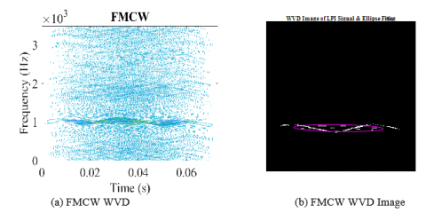
Figure 4. FMCW WVD and Image Transformation, SNR=0 dB
Figure 5. Frank coded waveform WVD and image transformation, SNR = 0 dB
Simulations are performed for 8 types of LPI radar signal waveforms. 1000 Monte-Carlo simulations are performed and detection is decided both for ACF peak determination and the orientation angle value. At least two peak determination is necessary, and orientation angle needs to be in the range $-60^{\circ}<\theta<60^{\circ}$. Simulation results based on ACF are given in Table 4. Detection probability based on orientation angle is given in Table 5. Energy detection (ED) performance is also analyzed to compare the results. The threshold value of energy detection is calculated by the formula given in Eq. (32) for $p f a=0.05$ and antenna number $M=1$. Simulation results of (ED) are given in Table 6.
Table 4. Detection probability of proposed method with ACF
|
Signal SNR (dB) |
FMCW |
BPSK |
Polyphase Barker |
Frank |
T1 |
T3 |
P1 |
P3 |
|
0 |
100 |
100 |
100 |
100 |
100 |
100 |
100 |
100 |
|
-3 |
100 |
100 |
100 |
100 |
100 |
100 |
100 |
100 |
|
-5 |
100 |
100 |
100 |
100 |
100 |
100 |
100 |
100 |
|
-6 |
100 |
100 |
100 |
100 |
100 |
100 |
100 |
99.7 |
|
-7 |
100 |
100 |
99.6 |
94.9 |
100 |
100 |
96.1 |
95.3 |
|
-8 |
99.8 |
100 |
86 |
33.8 |
99.8 |
100 |
35 |
34.8 |
|
-9 |
84.9 |
97.5 |
22.3 |
2.1 |
80.1 |
92.9 |
1.5 |
2.2 |
|
-10 |
35.4 |
70.8 |
2.2 |
0.1 |
29.2 |
56.5 |
0.1 |
0.1 |
Table 5. Detection probability of proposed method with orientation angle
|
Signal SNR (dB) |
FMCW |
BPSK |
Polyphase Barker |
Frank |
T1 |
T3 |
P1 |
P3 |
|
0 |
100 |
100 |
100 |
100 |
100 |
100 |
100 |
100 |
|
-3 |
100 |
95.7 |
89.2 |
100 |
74.7 |
100 |
100 |
100 |
|
-5 |
100 |
34.3 |
15.2 |
95.9 |
7.1 |
95.4 |
100 |
97.5 |
|
-6 |
95.4 |
11.2 |
3.9 |
67.8 |
1.7 |
67 |
97.3 |
81.3 |
|
-7 |
74.5 |
2.6 |
0.6 |
27.8 |
0.5 |
26.6 |
80.8 |
39.7 |
|
-8 |
29.4 |
0.2 |
0.1 |
5.2 |
0.1 |
5.3 |
43.3 |
9.8 |
|
-9 |
4.1 |
0 |
0.1 |
0.6 |
0 |
1 |
12 |
1.3 |
|
-10 |
1.6 |
0 |
0 |
0 |
0 |
0.1 |
3.8 |
0.4 |
Table 6. Energy detection probability with pfa=0.05
|
Signal SNR (dB) |
FMCW |
BPSK |
Polyphase Barker |
Frank |
T1 |
T3 |
P1 |
P3 |
|
0 |
100 |
100 |
100 |
100 |
100 |
100 |
100 |
100 |
|
-1 |
100 |
100 |
100 |
100 |
100 |
100 |
100 |
100 |
|
-2 |
100 |
100 |
100 |
100 |
100 |
100 |
100 |
100 |
|
-3 |
100 |
100 |
100 |
100 |
100 |
100 |
100 |
100 |
|
-4 |
95.5 |
97.5 |
97.1 |
97.8 |
96.2 |
96.9 |
95.9 |
97 |
|
-4.5 |
0 |
0.1 |
0 |
0 |
0.1 |
0.2 |
0 |
0.2 |
|
-6 |
0 |
0 |
0 |
0 |
0 |
0 |
0 |
0 |
|
-7 |
0 |
0 |
0 |
0 |
0 |
0 |
0 |
0 |
In this paper, a non-cooperative detection technique for LPI radar waveforms has been represented. FMCW and seven different types of PSK-modulated LPI waveforms (including BPSK, Polyphase Barker, Frank, P1, P3, T1, and T3) are considered in the analysis. The detection algorithm uses both the autocorrelation function characteristics and extracted features from the Wigner-Ville Distribution of the intercepted signal. The ACF-based detection takes advantage of the periodic structure of continuous wave LPI radar signals. On the other hand, in the WVD analysis, the orientation angle of WVD based image is used as a detection decision criterion. Connected Component Labeling algorithm used to eliminate noise pixels in the WVD image. The generation of LPI radar signals and the fundamental analysis are carried out using MATLAB for different SNR conditions. Energy detection method simulations were also carried out to compare detection performances. Simulation results show that both methods in the proposed solution give good results under low SNR conditions. Until -7 dB SNR, detection is possible for all LPI waveforms with an ACF-based detection algorithm. Compared with the energy detection, simulation results show that the proposed solution performs better.
We plan to extend time-frequency analysis to the application of radar signal parameter extraction and classification of waveforms for the future work. Also, this provides intelligent jamming techniques for the EW systems. Thus, jamming methods against LPI radars will be studied as a second future projection.
[1] Schrick, G., Wiley, R.G. (1990). Interception of LPI radar signals. In IEEE international conference on radar, pp. 108-111. https://doi.org/10.1109/RADAR.1990.201147
[2] Kishore, T.R., Rao, K.D. (2017). Automatic intrapulse modulation classification of advanced LPI radar waveforms. IEEE Transactions on Aerospace and Electronic Systems, 53(2): 901-914. https://doi.org/10.1109/TAES.2017.2667142
[3] Pace, P.E. (2009). Detecting and classifying low probability of intercept radar. Artech house.
[4] Walden, M.C., Pollard, R.D. (1993). On the processing gain and pulse compression ratio of frequency hopping spread spectrum waveforms. In Conference Proceedings National Telesystems Conference, IEEE, pp. 215-219. https://doi.org/10.1109/NTC.1993.292983
[5] Kelley,K.J.,Weber, C.L. (1985). Principles of spread spectrum radar. In: Milcom, IEEE, Military Communications Conference, 3: 586-590. https://doi.org/10.1109/MILCOM.1985.4795104
[6] Scholtz, R. (1982). The origins of spread-spectrum communications. IEEE transactions on Communications, 30(5): 822-854. https://doi.org/10.1109/TCOM.1982.1095547
[7] Ghadimi, G., Norouzi, Y., Bayderkhani, R., Nayebi, M.M., Karbasi, S.M. (2020). Deep learning-based approach for low probability of intercept radar signal detection and classification. Journal of Communications Technology and Electronics, 65: 1179-1191. https://doi.org/10.1134/S1064226920100034
[8] Palo, F.D., Galati, G., Pavan, G., Wasserzier, C., Savci, K. (2020). Introduction to noise radar and its waveforms. Sensors, 20(18): 5187. https://doi.org/10.3390/s20185187
[9] Shirude, N.S. (2016). Increase accuracy in range estimation of radar system. In: 2016 International Conference on Communication and Signal Processing (ICCSP) IEEE, pp: 1868-1872. https://doi.org/10.1109/ICCSP.2016.7754494
[10] Majumder, U.K., Bell, M.R., Rangaswamy, M. (2013). A novel approach for designing diversity radar waveforms that are orthogonal on both transmit and receive. In: IEEE Radar Conference (RadarCon13), pp: 1-6. https://doi.org/10.1109/RADAR.2013.6586073
[11] Shirude, N., Gofane, M., Panse, M.S. (2014). Design and simulation of RADAR transmitter and receiver using direct sequence spread spectrum. IOSR Journal of Electronics and Communication Engineering e-ISSN, 2278-2834. https://doi.org/10.9790/2834-09365665
[12] Ammar, K., Ben Haj Belkacem, O., Bouallegue, R. (2020). DSSS transmission technique to joint radar sensing and wireless communications in V2V system. In Web, Artificial Intelligence and Network Applications: Proceedings of the Workshops of the 34th International Conference on Advanced Information Networking and Applications. (WAINA-2020) Springer International Publishing, pp: 376-385. https://doi.org/10.1007/978-3-030-44038-1_34
[13] Tian, R., Zhang, G., Zhou, R., Dong, W. (2016). Detection of polyphase codes radar signals in low SNR. Mathematical Problems in Engineering. https://doi.org/10.1155/2016/1382960
[14] Hoang, L.M., Kim, M.J., Kong, S.H. (2019). Deep Learning Approach to LPI Radar Recognition. In:2019 IEEE Radar Conference (RadarConf), pp. 1-8. https://doi.org/10.1109/RADAR.2019.8835772
[15] Jawad, M., Iqbal, Y., Sarwar, N., Siddiqui, F.A. (2019). Modulation characteristics analysis of the LPI radar pulses under non-cooperative estimation. In:2019 16th International Bhurban Conference on Applied Sciences and Technology (IBCAST) IEEE, pp: 943-946. https://doi.org/10.1109/IBCAST.2019.8666963
[16] Sachin, A.R., Ambat, S.K., Hari, K.V.S. (2017). Analysis of intra-pulse frequency-modulated, low probability of interception, radar signals. Sādhanā, 42: 1037-1050. https://doi.org/10.1007/s12046-017-0672-2
[17] Lundén, J. (2009). Spectrum sensing for cognitive radio and radar systems. Signaalinkäsittelyn Ja Akustiikan Laitos.
[18] Vlok, J.D. (2014). Detection of direct sequence spread spectrum signals. Doctoral dissertation, University of Tasmania. https://eprints.utas.edu.au/22401/1/whole-Vlok-thesis-2014.pdf, accessed on February 8 2023.
[19] Tang, X., Jiang, B., Zhang, C., He, Y. (2006). Detection and Parameter Estimiation of LPI Signals in Passive Radar. In: 2006 CIE International Conference on Radar IEEE, pp: 1-4. https://doi.org/10.1109/ICR.2006.343238
[20] Wiley, R. (2006). ELINT: The interception and analysis of radar signals. Artech.
[21] Chilukuri, R.K., Kakarla, H.K., Subbarao, K. (2020). Estimation of modulation parameters of LPI radar using cyclostationary method. Sensing and Imaging, 21: 1-20.
https://doi.org/10.1007/s11220-020-00313-3
[22] Shyamsunder, M., Subbarao, K., Regimanu, B., Teja, C. K. (2016). Estimation of modulation parameters for LPI radar using quadrature mirror filter bank. In:2016 IEEE Uttar Pradesh Section International Conference on Electrical, Computer and Electronics Engineering (UPCON), pp: 239-244. https://doi.org/10.1109/UPCON.2016.7894659
[23] Keerthi, Y., Bhatt, T.D. (2015). LPI radar signal generation and detection. Int. Res. J. Eng. Technol, 2(7): 721-727.
[24] Copeland, D.B., Pace, P.E. (2002). Detection and analysis of FMCW and P-4 polyphase LPI waveforms using quadrature mirror filter trees. In: 2002 IEEE International Conference on Acoustics, Speech, and Signal Processing, 4: IV-3960. https://doi.org/10.1109/ICASSP.2002.5745524
[25] Gupta, A., Rai, A.B. (2019). Feature extraction of intra-pulse modulated LPI waveforms using STFT. In:2019 4th International Conference on Recent Trends on Electronics, Information, Communication & Technology (RTEICT) IEEE, pp: 742-746. https://doi.org/10.1109/RTEICT46194.2019.9016799
[26] Shyamsunder, M., Rao, K.S. (2017). Time Frequency Analysis of LPI radar signals using Modified S transform. Int J Electron Eng Res, 9(8): 1267-1283.
[27] Konopko, K. (2007). A detection algorithm of LPI radar signals. In Signal Processing Algorithms, Architectures, Arrangements, and Applications SPA 2007 IEEE, pp: 103-108. https://doi.org/10.1109/SPA.2007.5903308
[28] Nuhoglu, M.A., Alp, Y.K., Akyon, F.C. (2020). Deep learning for radar signal detection in electronic warfare systems. In: 2020 IEEE Radar Conference (RadarConf20), pp: 1-6. https://doi.org/10.1109/RadarConf2043947.2020.9266381
[29] Wan, T., Jiang, K., Tang, Y., Xiong, Y., Tang, B. (2020). Automatic LPI radar signal sensing method using visibility graphs. IEEE Access, 8: 159650-159660. https://doi.org/10.1109/ACCESS.2020.3020336
[30] Lundén, J., Koivunen, V. (2007). Automatic radar waveform recognition. IEEE Journal of Selected Topics in: Signal Processing, 1(1): 124-136. https://doi.org/10.1109/JSTSP.2007.897055
[31] Wang, H., Diao, M., Gao, L. (2018). Low probability of intercept radar waveform recognition based on dictionary leaming. In: 2018 10th International Conference on Wireless Communications and Signal Processing (WCSP) IEEE, pp: 1-6. https://doi.org/10.1109/WCSP.2018.8555906
[32] Zhang, M., Liu, L.T., Diao, M. (2016). LPI radar waveform recognition based on time-frequency distribution. Sensors, 16(10): 1682. https://doi.org/10.3390/s16101682
[33] Kocaadam, E., Özkazanç, Y. (2010). Classification of LPI radar signals via eigenimage approach. In: IEEE 15th Signal Processing and Communications Applications Conference, pp: 17-18. https://doi.org/10.1109/SIU.2007.4298644
[34] Wang, C., Gao, H., Zhang, X. (2016). Radar signal classification based on auto-correlation function and directed graphical model. In: IEEE International Conference on Signal Processing, Communications and Computing (ICSPCC), pp: 1-4. https://doi.org/10.1109/ICSPCC.2016.7753693
[35] Boashash, B. (2015). Time-frequency signal analysis and processing: a comprehensive reference. Academic press.
[36] Priyanka, K.L., Ravichandran, S., Venkatram, N. (2014). Pulse compression techniques for target detection. International Journal of Computer Applications, 96(22): 23-28.
[37] Levanon, N., Mozeson, E. (2004). Radar signals. John Wiley Sons.
[38] Stimson, G.W. (1998). Introduction to airborne radar. SciTech Publishing, Inc.
[39] Leukhin, A.N., Voronin, A.A., Merzlyakov, A.S. (2020). Application of multiphase sequences with low sidelobe level in synthetic aperture radar. In: Journal of Physics: Conference Series IOP Publishing, 1679(2): 022042. https://doi.org/10.1088/1742-6596/1679/2/022042
[40] Singh, S.P. Subba Rao, K. (2010). Thirty-two phase sequences design with good autocorrelation properties. Sadhana, 35: 63-73. https://doi.org/10.1007/s12046-010-0001-5
[41] . Mahafza, B. (2013). Radar systems analysis and design using MATLAB®
[42] Miller, S., Childers, D. (2012). Probability and random processes: With applications to signal processing and communications. Academic Press.
[43] Burel, G. (2000). Detection of spread spectrum transmissions using fluctuations of correlation estimators. In: IEEE Int. Symp. on Intelligent Signal Processing and Communication Systems (ISPACS'2000) Honolulu, Hawaii, USA, 11: B8.
[44] Ma, Z., Huang, Z., Lin, A., Huang, G. (2020). LPI radar waveform recognition based on features from multiple images. Sensors, 20(2): 526. https://doi.org/10.3390/s20020526
[45] Wang, Y., Rao, Y., Xu, D. (2020). Multichannel maximum-entropy method for the Wigner-Ville distribution. Geophysics, 85(1): 25-31. https://doi.org/10.1190/geo2019-0347.1
[46] Kay, S.M. (1998). Fundamentals of statistical signal processing: detection theory. Prentice-Hall PTR.
[47] Luo, J., Zhang, G., Yan, C. (2022). An Energy detection-based spectrum-sensing method for cognitive radio. Wireless Communications and Mobile Computing https://doi.org/10.1155/2022/3933336
[48] Dillencourt, M.B., Samet, H., Tamminen, M. (1992). A general approach to connected-component labeling for arbitrary image representations. Journal of the ACM (JACM), 39(2): 253-280. https://doi.org/10.1145/128749.128750
[49] He, L., Ren, X., Gao, Q., Zhao, X., Yao, B., Chao, Y. (2017). The connected-component labeling problem: A review of state-of-the-art algorithms. Pattern Recognition, 70: 25-43. https://doi.org/10.1016/j.patcog.2017.04.018
[50] Rocha, L., Velho, L., Carvalho, P.C.P. (2002). Image moments-based structuring and tracking of objects. In: Proceedings. XV Brazilian Symposium on Computer Graphics and Image Processing IEEE, pp: 99-105. https://doi.org/10.1109/SIBGRA.2002.1167130