A Hybrid Firefly Algorithm–Bayesian Neural Network Framework for Inverse Weibull Parameter Estimation and Wind Energy Potential Assessment Using Generalized Three-Way Decision Ranking

The methodology to be used to assess wind power generation potential and the cost analysis of the economic aspects of the installation of the turbine of wind within various tower height is as suggested and shown in Figure 1, which shows the step-by-step process. According to this framework and equations available in the computational analysis subsection the analysis was conducted.

tu_pian_1.png

Figure 1. Workflow of current research

2.1 Wind speed dataset description and preprocessing

The daily mean wind-speed data were collected from the Central Pollution Control Board, Government of India, from four monitoring stations in the state of Andhra Pradesh namely Visakhapatnam, Rajamahendravaram, Amaravati and Tirupati. The following periods were all used for analysis: The data for the three cities, namely Visakhapatnam, Rajamahendravaram and Tirupati, were collected during four years from 1 January 2018 to 31 December 2021 (raw N = 1461 daily observations per city). The dates are 1 January 2020 to 31 December 2021 (two years; raw N = 731 daily observations). After quality control process and interpolation of the gaps in the data, the final sample size for distribution fitting were N = 1461 (Visakhapatnam, Rajamahendravaram and Tirupati) and N = 731 (Amaravati).

2.1.1 Missing data handling

The raw wind-speed series were screened for missing and invalid observations. Missing observations represented 15 records (1.0%) in Visakhapatnam, 18 records (1.2%) in Rajamahendravaram, 12 records (0.8%) in Tirupati, and 9 records (1.2%) in Amaravati. Short gaps were corrected using linear interpolation to preserve continuity of the daily mean wind-speed series. A quality-control rule was established whereby gaps of seven or more consecutive days would be excluded from subsequent distribution-fitting analyses. However, no such long gaps occurred in any of the four datasets. Consequently, no observations were excluded, and the number of excluded days was zero for all study sites.

2.1.2 Outlier screening and treatment

Outliers were screened on a monthly basis to respect seasonal variability. A data point was flagged as an outlier if it deviated by more than 3 standard deviations from the corresponding monthly mean. This procedure flagged 7 observations (0.5%) in Visakhapatnam, 10 (0.7%) in Rajamahendravaram, 6 (0.4%) in Tirupati, and 4 (0.5%) in Amaravati. Flagged values were manually checked against neighboring days and the overall seasonal pattern. When a flagged value was clearly inconsistent with local temporal context (indicative of measurement error), it was treated as missing and handled using the missing-data protocol described above; otherwise, it was retained to avoid removing genuine high-wind events that are important for tail-sensitive modelling. The numbers corrected (treated as missing and then interpolated) were 3 (0.2%) in Visakhapatnam, 5 (0.3%) in Rajamahendravaram, 2 (0.1%) in Tirupati, and 2 (0.3%) in Amaravati.

2.1.3 Normalization for machine learning

For the BNN component, wind-speed values were normalized using z-score standardization (subtract mean and divide by standard deviation), computed on the training subset only and then applied to validation/test subsets to avoid data leakage. Distribution fitting for the inverse Weibull and other parametric models was conducted on the original physical units (m/s) to retain interpretability.

2.1.4 Influence of preprocessing on distribution fitting

Variance, tail behavior and extreme-value representation effects can be caused by the preprocessing procedures which may affect the distribution fitting. Only observations that were identified as either not observed or clearly erroneous after the context was verified were corrected in order to minimize potential bias. The percent of interpolated and corrected observations were very small (less than 1.5% of observations) for all four sites, so the effect of preprocessing on the final estimates of the parameters is likely to be minimal. The percentages of corrected observations are explicitly reported to give transparency on data quality and the effects of data preprocessing.

2.2 Inverse Weibull parameters computation

The evaluation of wind energy is based on the modeling of the wind speed through the inverse Weibull distribution. Eight estimation techniques are compared, such as moments method (MoM), EPFM, maximum likelihood method (MLM), energy density method (EDM), Rayleigh, FFA–BNN, and novel NEPFM [22], and the Rayleigh technique is coded in MATLAB [25]. The inverse Weibull PDF and CDF given below are used to obtain the power potential of wind [23].

$g\left( v \right)=\left( \frac{a}{b} \right){{\left( \frac{v}{b} \right)}^{-\left( a+1 \right)}}{{e}^{-{{\left( \frac{v}{b} \right)}^{-a}}}},~v>0$   (1)

$G\left( v \right)=1-{{e}^{-{{\left( \frac{v}{b} \right)}^{-a}}}}$        (2)

In this case, $g\left( v \right)$ is the probability density function of the speed of the wind at the speed v (in m/s), and $G\left( v \right)$ is the CDF of v. The dimensionless shape parameter a determines the distribution shape, while the scale parameter b is expressed in the same units as v (m/s).

$\text{MFV}=a{{\left( \frac{b}{a+1} \right)}^{1/a}}$         (3)

$V{{C}_{\text{max}}}=a{{\left( \frac{b}{a-2} \right)}^{1/a}}$        (4)

The inverse Weibull distribution was chosen because it is flexible in heavy tailed behavior of wind speeds and it can capture the nature of failure rates that is applicable in the variability of wind energy. The inverse Weibull distribution has better ability to represent extreme regimes of wind and skewed distributions typical of coastal and semi-arid areas compared to other distributions like Gamma, Lognormal or Rayleigh. In prior research, it was shown that Weibull models have the advantage of reflecting tail risk behavior of low-probability high-impact wind events, which is essential in the stable estimation of wind power density and turbine performance. Also, the inverse Weibull formulation can be integrated with reliability-based models and decision-theoretic models, like the generalized three-way decision (G3WD) scheme, used in this paper consistent with that. The Gamma distribution provides analytical simplicity, but can be inaccurate in estimating the dispersion in tails of heterogeneous wind regimes, and thus is less accurate in power density estimation. Thus, inverse Weibull distribution was chosen as a more appropriate probabilistic model of the variability of the wind speed in the chosen sites. A key condition for selecting the appropriate wind evaluation methods and WPP assessment is the accuracy of the wind power potential assessment, especially in the case of wind power systems located in locations with different wind regimes. The present study focuses exclusively on the inverse Weibull distribution and compares alternative parameter-estimation methods for this distribution rather than comparing different probability-distribution families. The objective is to determine which estimation method provides the most accurate and reliable inverse Weibull parameter estimates for wind-resource assessment. Accordingly, the comparative analysis is performed using relative power-density error (RPDE), root-mean-square error (RMSE), PDF and CDF goodness-of-fit measures, and the G3WD ensemble decision framework. The superiority of a particular estimation method is therefore assessed according to its overall performance across these evaluation criteria rather than through comparisons with alternative probability distributions. To ensure consistency throughout the manuscript, the inverse Weibull distribution is parameterized using a unified notation. The shape parameter is denoted by a, and the scale parameter is denoted by b. This notation is used consistently in all analytical derivations, numerical algorithms, and result tables. Any alternative symbols appearing in intermediate derivations or prior literature are mapped to this notation for clarity and comparability across methods.

The FA is an algorithm which is based on population and is meta-heuristic optimization that is inspired by the system of bioluminescent communication of fireflies [13]. Fireflies in the wild use repetitive and pulsating lights to signal mating, keep predators away and aid in foraging [14]. The main idea of FA is that the lower-intensity fireflies are drawn to brighter ones, which is a simulation of movement to optimum solutions in the search space. The problem landscape influences light intensity, which diminishes with the distance, and mathematically linked with the objective function to be optimized [8, 16]. Here the brightness values are a measure of how fit a solution is and the movement of the fireflies is a measure of the exploration of the solution space. The FA is subject to three rules (1) Unisex attraction occurs in all cases; (2) The degree of sexual attraction is directly related to brightness, and when there is an increase in distance, and (3) The quality of the solutions is proportional to the brightness. These values allow creating a balance between exploration and exploitation, which allows efficient international search. The strength and flexibility of FA have been tested and proven through multiple works, and the performance of FA proves to be better compared to PSO, GA, Ant Colony Optimization (ACO), Simulated Annealing (SA) and Harmony Search Algorithm (HSA) in diverse optimization problems, such as structural design, economic load dispatch problems, etc. [16, 32-34]. FA is a good choice due to its flexibility and good convergence properties, which offer a sound skeleton towards the solution of complex, data-driven optimization and classification problems. The attractiveness role of FA may be defined as follows:

$\beta \left( r \right)={{\beta }_{0}}\exp \left( -\gamma {{r}^{2}} \right)$       (18)

where, $r$ is the space that is located between any pair of fireflies, ${{\beta }_{0}}$ is attraction at $r=0$ (in this work 1), and $\gamma$ is a coefficient of absorption that regulates the decline of the intensity of light (in this work 1). A Cartesian or Euclidean space that lies between every two fireflies $i$ and $j~$at points x_i and ${{x}_{j}}$ respectively could be clarified as follows:

$r_{i j}=\left\|x_i-x_j\right\|=\sqrt{\sum_{k=1}^d\left(x_{i, k}-x_{j, k}\right)^2}$       (19)

where, d is a symbol for the problem-dimension. The firefly-migration i, to a more highlighted firefly j, is represented in Eq. (20):

$x_i^{t+1}=x_i^t+\beta_0 \exp \left(-\gamma r_{i j}^2\right)\left(x_j^t-x_i^t\right)+\alpha\left(\operatorname{rand}-\frac{1}{2}\right)$        (20)

6.1 Relative power-density error

The RPDE serves as an accuracy metric for time-series forecasts, widely used in modeling wind resources, solar inputs, and power consumption patterns. RPDE measures the difference between estimated and measured power density (usually in megawatts/square kilometer) in a given region or location. The computation of the RPDE is as:

$RPDE=\frac{\left( {{q}_{pdf}}-q \right)}{q}\times 100$        (23)

In this case, ${{q}_{pdf}}$ refers to the density of wind power calculated with the help of the method under consideration, and $q$ is the density of the power calculated by directly referring to the data measured. The approach with minimum RPDE is considered the most precise one to estimate power density.

${{P}_{pdf}}=\frac{1}{2}\rho {{a}^{3}}\text{ }\!\!\Gamma\!\!\text{ }\left( 1-\frac{3}{b} \right)$         (24)

$P=\frac{1}{2} \rho \bar{v}^3$       (25)

It should be noted that two different wind-power-density quantities are considered in this study. The theoretical model-based wind power density is obtained from the distributional third moment, $E\left( V{}^\text{3} \right).$ For the Inverse Weibull distribution, the r-th theoretical moment exists only when the shape parameter satisfies $a>r;$ therefore, the theoretical third moment is finite only when $a>3.$ When the fitted shape parameter satisfies $a\le 3,$ the theoretical third-moment expression is not finite and is not used for interpretation. In those cases, wind power density is evaluated using the empirical finite-sample mean of the observed cubic wind speeds, $\left( 1/n \right)\Sigma V{}^\text{3}.$ Accordingly, the RPDE values reported in this study compare empirical finite-sample wind-power-density estimates rather than divergent theoretical moments of the fitted Inverse Weibull distribution.

6.2 Root-mean-square error

RMSE helps in quantifying the root that is square, of the total squared variations among the predicted values and experimental values. A lower RMSE value means more accurate method of estimation.

$RMSE={{\left( \frac{1}{na}\underset{i=1}{\overset{na}{\mathop \sum }}\,{{\left( {{y}_{i}}-{{w}_{i}} \right)}^{2}} \right)}^{1/2}}$        (26)

6.3 Moments method

The method depends on numerically iterating the following two equations, assuming that the sample mean $\bar{u}$ and SD $\left( \sigma  \right)$ of the speed of the wind data are known.

$\bar{u}=\mathrm{a} \Gamma\left(1-\frac{1}{b}\right)$        (27)

$\sigma =\text{a}{{\left[ \text{ }\!\!\Gamma\!\!\text{ }\left( 1-2/b \right)-{{\text{ }\!\!\Gamma\!\!\text{ }}^{2}}\left( 1-1/b \right) \right]}^{1/2}}$      (28)

After the shape parameter a is determined by solving the moment equations numerically, the scale parameter b is calculated using the corresponding analytical expression. In this study, a and b denote the inverse Weibull shape and scale parameters, respectively.

$\hat{\mathrm{a}}=\frac{\bar{u}}{\Gamma(1-1 / b)}$          (29)

$\bar{u}=\frac{1}{n} \sum_{i=1}^n u_i$      (30)

$\sigma=\left[\frac{1}{n-1} \sum_{i=1}^n\left(u_i-\bar{u}\right)^2\right]^{1 / 2}$        (31)

where, $\text{ }\!\!\Gamma\!\!\text{ }$(⋅) denotes the Gamma function, defined by:

$\text{ }\!\!\Gamma\!\!\text{ }\left( z \right)=\mathop{\int }_{0}^{\infty }{{t}^{,z-1}}{{e}^{-t}},dt,\text{ }\!\!~\!\!\text{ }z>0$       (32)

The Gamma function appears in the analytical expressions of the moments of the inverse Weibull distribution and is used in the estimation of the shape and scale parameters through the method of moments.

6.4 Method of energy density

This approach is expressed as the approach of power density as well; and it employs the factor of the energy pattern (${{E}_{pf}}$) to determine the measure of shape.

$\overline{{{u}^{3}}}=\frac{1}{n}\times \underset{i=1}{\overset{n}{\mathop \sum }}\,{{\left( {{u}_{i}} \right)}^{3}}$        (33)

${{E}_{pf}}=\frac{\overline{{{u}^{3}}}}{{{u}^{3}}}$       (34)

The shape factor has to be obtained by the following equation, numerically:

${{E}_{pf}}=\frac{\text{ }\!\!\Gamma\!\!\text{ }\left( 1-\frac{3}{a} \right)}{{{\text{ }\!\!\Gamma\!\!\text{ }}^{3}}\left( 1-\frac{1}{a} \right)}$          (35)

After the shape parameter a is determined numerically from the energy-pattern factor equation, the scale parameter b is then calculated using the corresponding scale-parameter expression.

6.5 Method of maximum likelihood estimation

This method of maximum likelihood estimation (MLE) involves a large amount of numerical iteration. The estimation on the measures of shape and scale of inverse distribution of Weibull is then given below:

$a={{\left[ \frac{\mathop{\sum }_{i=1}^{n}u_{i}^{k}\text{ln}\left( {{u}_{i}} \right)}{\mathop{\sum }_{i=1}^{n}u_{i}^{b}}-\frac{\mathop{\sum }_{i=1}^{n}\text{ln}\left( {{u}_{i}} \right)}{n} \right]}^{-1}}$      (36)

$b={{\left( \frac{1}{n}\underset{i=1}{\overset{n}{\mathop \sum }}\,u_{i}^{b} \right)}^{1/b}}$         (37)

6.6 Method of energy pattern factor

The energy pattern factor method estimates the inverse Weibull shape and scale parameters using the relationship between wind-speed moments and wind-power density. In this study, the energy pattern factor is defined as:

$E_{p f}=\frac{E\left(V^3\right)}{(E(\bar{V}))^3}$         (38)

where, V denotes wind speed. For the inverse Weibull distribution with shape parameter a and scale parameter b, the r-th raw moment is given by:

$E\left( {{V}^{r}} \right)={{b}^{r}}\Gamma \left( \frac{1-r}{a} \right),~~a>r$        (39)

Therefore, the third moment exists only when a > 3. Substituting the first and third moments into the definition of the energy pattern factor gives:

$\overset{}{\mathop{u}}\,=\frac{\Gamma \left( 1-\frac{3}{a} \right)}{{{\left[ \Gamma \left( 1-\frac{1}{a} \right) \right]}^{3}}},~~a>3$         (40)

The shape parameter a is obtained by solving this nonlinear equation numerically. After a is estimated, the scale parameter $b$ is calculated from the sample mean wind speed $\bar{v}$ as: $b=\frac{\bar{v}}{\Gamma\left(1-\frac{1}{a}\right)}$. This formulation ensures that the energy pattern factor method is consistent with the inverse Weibull distribution adopted in this study. The symbols $a$ and $b$ are used throughout the manuscript to denote the shape and scale parameters, respectively.

6.7 Energy pattern factor method of Sathyajith

Energy pattern factor method of Satyajit (EPFMS) gives a means of the measures-approximation of the inverse Weibull distribution via the employment of the factor of energy pattern $({{E}_{pf.}}$). In the EPFMS method, the inverse Weibull shape parameter a is estimated from the energy-pattern factor. Once a is obtained, the scale parameter b is calculated using the same unified parameter notation:

$a=3.957\times E_{pf}^{-0.898}$       (41)

After the determination of the measure of shape a, that of scale b is then calculated as shown by Eq. (39).

6.8 Method of novel energy pattern factor

This technique represents an approximate version of the energy density method as given in Eq. (19). The parameters of distribution are calculated as follows:

$b=\frac{{{b}_{4}}E_{pf}^{4}+{{b}_{3}}E_{pf}^{3}+{{b}_{2}}E_{pf}^{2}+{{b}_{1}}{{E}_{pf}}+{{b}_{0}}}{{{c}_{4}}E_{pf}^{4}+{{c}_{3}}E_{pf}^{3}+{{c}_{2}}E_{pf}^{2}+{{c}_{1}}{{E}_{pf}}+{{c}_{0}}}$       (42)

$a=\frac{{{U}_{m}}\left( {{b}^{2}}+{{c}_{1}}b+{{c}_{0}} \right)}{{{b}^{2}}+{{d}_{1}}b+{{d}_{0}}}$         (43)

The coefficients presented were derived through curve fitting [23].

6.9 Rayleigh distribution

This method provides relatively simple analytical expressions and can be solved explicitly. In this specific issue of the inverse distribution of Weibull, For the Rayleigh baseline formulation, the inverse Weibull shape parameter is fixed at a = 3, and the corresponding scale parameter is denoted consistently by b:

$b=\frac{2{{U}_{m}}}{\sqrt{\pi }}$          (44)

6.10 Firefly Algorithm–Bayesian neural network

FA parameters were chosen through empirical research and sensitivity analysis that preceded the main research to provide a stable convergence and efficiency of computation. The coefficient of attractiveness was adjusted to ${{\beta }_{0}}=1.0$ to ensure sufficient attraction between candidate solutions, while the light absorption coefficient was fixed at $\gamma =1.0$ to control the decay of attractiveness with distance. The randomization parameter $\alpha =0.2$ was selected to maintain adequate exploration of the search space during early iterations while enabling gradual convergence through adaptive reduction using ${{\alpha }_{t+1}}=0.97{{\alpha }_{t}}$. The size of the population and the number of generations were selected in order to compromise between the quality of solutions and the complexity of computations. It was observed that the following parameter values gave the stable optimization performance in various experimental runs as shown in Algorithm 1.

The loss function in FFA–BNN is directly related to the inverse Weibull likelihood. The fitted pdf value $f\left( {{v}_{i}};\text{ }\!\!~\!\!\text{ }a,b \right)$ is calculated for each observed wind speed vi based on the same Inverse Weibull formulation defined in section 2.2. Maximizing or, alternatively, minimizing the negative log-likelihood, is equivalent to maximizing the total log-likelihood. This means the FA is not optimizing an unrelated objective function; it is optimizing the BNN weights in such a way that the resulting shape and scale parameters best maximize the likelihood that the shape and scale parameters found in the observed wind-speed data. The final FFA–BNN estimates are thus only for the shape parameter a and the scale parameter b. The inverse Weibull model has no third distributional parameter so it is neither estimated nor used.

FFA–BNN model was chosen to combine the advantageous features of the global optimization and probabilistic learning into the hybrid model. BNN can give good predictive accuracy as well as give concrete certainty of uncertainty in estimating the parameters, which is crucial in the assessment of wind resources where the environment variability is stochastic. The performance of BNNs, however, is very prone to hyperparameter setup and initialization. The FA was hence included in the list of optimization strategies (metaheuristic) capable of efficiently exploring the parameter space and escaping local minimum. The FA offers a high level of exploration-exploitation balance and has been shown to exhibit steady convergence to nonlinear parameter estimation problems as compared to other optimization methods, including PSO, GA or gradient descent variants. A combination of FFA and BNN provides better robustness to estimation, prediction, and also it is less sensitive to the noisy wind data. The proposed FFA–BNN approach is especially beneficial when the series of wind speeds is nonlinear and the variability is heteroscedastic between different seasons, the length of the series is short (as for some stations), and the uncertainty of the estimation is significant (when comparing the different parameter estimates and distributional fits). Classical estimators (such as MoM, EPF based and MLM) are efficient in cases where the underlying distribution is presumed to be correct, but can be less efficient in the case of violations of the assumptions of the distribution and may be more sensitive to local minima or to the inability of numerical iterations to converge to a solution, particularly when the likelihood surface is irregular. The FA has a global search method to enhance robustness against poor initializations and the Bayesian formulation allows uncertainty-aware estimation via probabilistic learning and not just point-estimates. In practice, we find that FFA–BNN outperforms conventional approaches when it can be used to consistently improve across multiple dimensions of evaluation (RPDE and RMSE, plus other distributional goodness-of-fit and information-criterion ranking measures), while conventional approaches are preferred when interpretation, limited computation, and closed-form estimation are more important.

6.11 Practical integration of generalized three-way decision with parameter estimation and model comparison

G3WD is not presented as an abstract theoretical extension in this study but is employed as a decision layer that integrates multiple performance indicators and transforms them into an actionable ranking of estimation methods. It should be emphasized that G3WD is not an estimation method, optimization algorithm, machine-learning model, or probability distribution. Rather, it is a post-estimation decision framework used to evaluate and classify the outputs of the competing parameter-estimation methods.

In this study, eight parameter-estimation methods are considered, namely MoM, EDM, EPFM, EPFMS, NEPFM, MLM, Rayleigh method, and the FFA–BNN. Each method produces estimates of the inverse Weibull shape parameter a and scale parameter b, from which the corresponding PDF, CDF, and performance measures are obtained.

For each study site, the estimation methods are evaluated using the same set of criteria described in Section 6, including RPDE, RMSE (PDF), RMSE (CDF), and goodness-of-fit statistics. Because different criteria may favor different methods, a multi-criteria decision framework is required to provide a unified assessment of overall performance. The G3WD framework therefore operates on the calculated performance measures and produces both a final ranking and a three-way decision classification.

The G3WD framework partitions the candidate methods into three decision regions:

POS: methods exhibiting superior overall performance and recommended for application.

BND: methods exhibiting intermediate or uncertain performance that may require additional evaluation before selection.

NEG: methods exhibiting comparatively weaker performance and therefore not recommended when superior alternatives are available.

The final classification is determined according to the G3WD procedures described in Section 3. The practical outcome is a ranked list of estimation methods together with a POS, BND, or NEG assignment for each method. Methods classified in the POS region are considered the most suitable for practical application, methods in the BND region are regarded as conditionally acceptable, and methods in the NEG region are considered less suitable when compared with higher-ranked alternatives.

The principal advantage of incorporating G3WD into the proposed framework is that model selection is not based on a single evaluation criterion. A method that performs well according to one metric may not necessarily perform best according to another. By integrating multiple performance indicators into a unified decision process, G3WD provides a more balanced and transparent assessment of estimation-method performance across different datasets and wind regimes. Consequently, the final rankings reported in this study should be interpreted as multi-criteria decision outcomes rather than conclusions derived from any individual metric alone.

The mean wind speed data of the selected four stations namely Visakhapatnam, Rajamahendravaram, Amaravati and Tirupati of Andhra Pradesh, India, has been analyzed for the day-wise period. The variations in wind speed at the four sites during the year are shown in Figure 4 in terms of monthly mean wind speed, to be used as a means of identifying the seasonal behaviour of the observed wind regime prior to distribution fitting. The monthly and annual standard deviations for the wind speed at the stations of Visakhapatnam, Rajamahendravaram, Amaravati and Tirupati respectively are summarized in Tables 1–4, which compare the variability structure of the four datasets and for model performance site-wise interpretation.

(a) Monthly variations of mean wind speed at Visakhapatnam

(b) Monthly mean wind speed variations at Rajamahendravaram

(c) Monthly mean wind speed variations at Amaravati

(d) Monthly mean wind speed variations at Tirupati

Figure 4. Monthly mean wind speed variations at four sites over four years

Table 1. Monthly and annual standard deviation of wind speed at Visakhapatnam

Table 2. Monthly and annual standard deviation of wind speed (m/s) at Rajamahendravaram

Table 3. Monthly and annual standard deviation of wind speed (m/s) at Amaravati

Table 4. Monthly and annual standard deviation of wind speed (m/s) at Tirupati

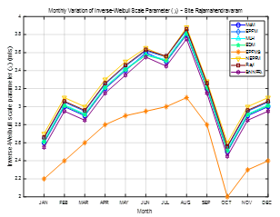
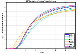
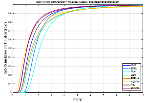
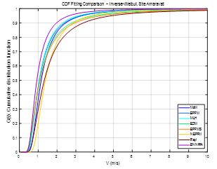
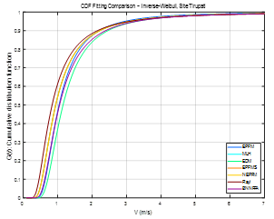
The variation in wind speed for each month of the year from the various stations is shown in Figure 5 for Rajamahendravaram, Amaravati and Tirupati and in Figure 6 for Visakhapatnam and Tirupati, the relationship between mean wind speed and standard deviation. Figures 7 and 8 display the monthly evolution of the inverse Weibull shape and scale parameters, respectively, while Figures 9 and 10 show the evolution of the fitted PDF and CDF curves, respectively, between the four study sites. The detailed tables of the inverse Weibull parameters estimated on monthly time steps were placed in Appendix for better logical flow of the results section. The inverse Weibull shape parameter a and scale parameter b for all estimation methods for all study sites are available in Appendix Tables A1–A4.

tu_pian_9.png

(a) Standard deviation of monthly wind speed at Rajamahendravaram

tu_pian_10.png

(b) Monthly wind speed variability at the Amaravati Site

tu_pian_11.png

(c) STD of monthly wind speed of the site Tirupati

Figure 5. Monthly wind speed variability across the three sites

tu_pian_12.png

(a) Linear relationship between average wind speed and standard deviation for the Visakhapatnam location

tu_pian_13.png

(b) Linear relationship between average wind speed and standard deviation for the Tirupati location

Figure 6. Linear dependence of the mean wind speed on the corresponding standard deviation for the two sites

tu_pian_14.png

(a) Site Visakhapatnam

tu_pian_15.png

(b) Site Rajamahendravaram

tu_pian_16.png

(c) Site Amaravati

tu_pian_17.png

(d) Site Tirupati

Figure 7. Variation per month of inverse measure of the shape of Weibull of four sites

tu_pian_18.png

(a) Site Visakhapatnam

tu_pian_19.png

(b) Site Rajamahendravaram

tu_pian_20.png

(c) Site Amaravati

tu_pian_21.png

(d) Site Tirupati

Figure 8. Monthly variation of inverse Weibull scale parameter of four study sites

tu_pian_22.png

(a) Site Visakhapatnam

tu_pian_23.png

(b) Site Rajamahendravaram

tu_pian_24.png

(c) Site Amaravati

tu_pian_25.png

(d) Site Tirupati

Figure 9. Distributional fitting comparison of wind speed data for the four locations

tu_pian_26.png

(a) Site Visakhapatnam

tu_pian_27.png

(b) Site Rajamahendravaram

tu_pian_28.png

(c) Site Amaravati

tu_pian_29.png

(d) Site Tirupati

Figure 10. Comparison of cumulative distribution function fits across the four study sites

The analysis was then conducted extensively on seven estimation methods comparing RPDE, RMSE and chi-square goodness-of-fit tests of each site. The comparative analysis was performed by RPDE, RMSE calculated using PDF and CDF. The RPDE results have been provided in Tables 5–8 for the town of Visakhapatnam, Rajamahendravaram, Amaravati and Tirupati respectively. The fitting results are given in PDF form in Tables 9–12 and in CDF form in Tables 13–16. The results presented here indicate that the hybrid FFA–BNN approach tends to yield more consistent results over locations and evaluation measures, while the conventional methods offer better performance in different locations and measures.

Table 5. Empirical finite-sample relative power-density error (RPDE) and wind regime profile for Visakhapatnam

Note: MoM = moments method; EPFM = energy pattern factor method; MLM = maximum likelihood method; EDM = energy density method; EPFMS: Energy Pattern Factor Method of Sathyajith; NEPFM: novel energy pattern factor method; FFA–BNN: Firefly Algorithm–Bayesian neural network.

Table 6. Empirical finite-sample relative power-density error (RPDE) and wind regime profile for Rajamahendravaram

Table 7. Empirical finite-sample relative power-density error (RPDE) and wind regime profile for Amaravati

Table 8. Empirical finite-sample relative power-density error (RPDE) and wind regime profile for Tirupati

Table 9. Probability density function (PDF)-based comparison for Visakhapatnam

Note: MoM = moments method; EPFM = energy pattern factor method; MLM = maximum likelihood method; EDM = energy density method; EPFMS: Energy Pattern Factor Method of Sathyajith; NEPFM: novel energy pattern factor method; FFA–BNN: Firefly Algorithm–Bayesian neural network; $\chi^2$: Chi-square statistic; RMSE: root-mean-square error.

Table 10. Probability density function (PDF)-based comparison for Rajamahendravaram

Table 11. Probability density function (PDF)-based comparison for Amaravati

Regarding a practical wind energy engineering point of view, better parameter estimation will result in the better prediction of wind power density and turbine performance features. Wind variability is a critical aspect of the wind modeling that is necessary to optimize turbine locating, predicting the energy production in the long-term, and mitigating financial risk posed by the renewable energy investments. The findings indicate that the hybrid FFA–BNN model offers consistency in predictive performance in heterogeneous geographical settings, implying that the technique is applicable to the real-world wind resource assessment problem where the environment is prone to uncertainty and is very dynamic.

Table 12. Probability density function (PDF)-based comparison for Tirupati

Table 13. Cumulative distribution function (CDF)-based comparison for Visakhapatnam

Table 14. Cumulative distribution function (CDF)-based comparison for Rajamahendravaram

Table 15. Cumulative distribution function (CDF)-based comparison for Amaravati

Table 16. Cumulative distribution function (CDF)-based comparison for Tirupati

Both algorithmic and practical explanations can describe why hybrid FFA–BNN approach has been proven to outperform the other two methods. Algorithms BNN gives a probabilistic model of learning that can model nondynamic relationships between wind speed measurements and parameter distribution values and also measures the uncertainty in the estimation of the parameters. The Bayesian formulation is more effective compared to deterministic optimization techniques in minimizing the risk of overfitting, and it has better levels of generalization, especially where wind data are diverse because of seasonal atmospheric variations. The FA also improves the work of models by globalizing the optimization of network parameters to enable the search process to avoid local minima usually faced during gradient-based learning. The FA has a mechanism, the adaptive attractiveness mechanism, which facilitates efficient exploration of the solution space, enhancing the stability of convergence as well as providing a reliable estimation of the inverse Weibull shape and scale parameters. Statistically, the hybrid model has smaller values of RMSE and RPDE since it can describe all central tendencies and tail variations in wind speed distributions. The classical methods of estimation like the MoM, MLM, and EPFM are based on static assumptions of analysis which do not necessarily reflect the complicated wind regimes of skewness and heteroscedastic variability. Conversely, the FFA–BNN model is a dynamic system to estimate parameter values depending on the observed data characteristics and imparts a better fitting capability to the PDF and the CDF models in all four study sites.

8.1 Site-wise performance breakdown of FFA–BNN and conditions of superiority

It should be noted that the aim of this study is not to check the superiority of the inverse Weibull distribution compared to other probability distributions like Gamma or Lognormal distribution but to see whether this distribution is the best choice. Instead, the aim is to compare the various parameter-estimation techniques in the inverse Weibull framework and determine which estimation technique yields the best overall performance from a point of view of RPDE, RMSE, PDF/CDF goodness-of-fit and the G3WD ensemble evaluation.

We summaries the results at each site in Table 17 and provide detailed performance tables for each site. As can be seen in Tables 5–8, across the four sites FFA–BNN has the best or most competitive RPDE performance. As demonstrated in Tables 9–12, the fitting accuracy of FFA–BNN is the lowest RMSE and highest goodness-of-fit among the corresponding site-level comparisons for PDF-based fitting accuracy. Compared to the empirical cumulative wind-speed distributions, presented in Tables 13–16, FFA–BNN has the best overall agreement in terms of fitting accuracy for the CDF. From these results, it is observed that the hybrid approach not only performs well in one criterion but also is stable across the various evaluation metrics used in RPDE, PDF fitting, CDF fitting and G3WD based decision ranking.

The distribution of wind speed for Visakhapatnam (coastal wind regime) has a seasonal variation in both the centre and the upper tail. When the conditions are like this, FFA–BNN gives the best overall agreement to the empirical distribution especially on PDF and CDF fitting accuracy. This suggests that the hybrid model would be appropriate for sites on the coast where seasonal variability and tail behavior are significant for the wind-energy assessment.

The month-to-month variation is seen to be higher for the standard deviation of the region of high variability than observed at other sites, as in the case of Rajamahendravaram. This variability can result in a less smooth estimation surface for the classical estimators. The FA is used to enhance the search process by mitigating the dependence of initial parameters and local minima to the search process, with the BNN component used to stabilize the estimation process in uncertain scenarios. The benefit of FFA–BNN is particularly pronounced at locations characterized by significant wind fluctuations and variability within each year, and by varying wind directions.

The length of wind-speed series is less for Amaravati when compared with the other sites. The shorter the data records, the more uncertain the estimation is, particularly in the case of methods that rely heavily on sample moments or likelihood estimation through iteration. The Bayesian part of FFA–BNN acts as a regularizing effect and the FA helps in finding the optimal inverse Weibull parameters. The good results of RPDE and RMSE for Amaravati thus justify the usefulness of FFA–BNN in limited sample situations.

The wind-speed pattern over Tirupati is different from the coastal and inland sites as it is the upland, terrain influenced regime. When the fitting of PDF/CDF is taken together with RPDE, then energy-pattern-factor-based methods are still useful baseline estimators, but FFA–BNN gives better overall distributional agreement. This validates the proposed method for a larger benefit when the objective of the evaluation goes beyond just error in wind power density, but also incorporates the distribution of fidelity.

FFA–BNN is empirically better than the base at large in cases where the wind-speed data has high intra-annual variability, heteroscedasticity, a short sample length, or where model selection requires using more than one of the RPDE, RMSE, PDF/CDF goodness-of-fit, or G3WD rankings. The results of the simpler estimators (EPFM, EPFMS, EDM and NEPFM) are, by comparison, not as stable across sites and across metrics as the hybrid FFA–BNN estimator, as can be seen from Tables 5–18.

As seen in Tables A1–A4, several of the values for shape parameters a are less than the threshold, a = 3. The parameter combinations for which the analytical third moment of the fitted inverse Weibull distribution is not finite for those parameter combinations. So, in general, the wind-power-density comparisons should be taken in terms of empirical finite-sample estimates of wind-speed cubed, specifically and not in terms of theoretical third-moment expressions of all fitted distributions.

The shape parameters fitted in Appendix Tables A1–A4 were checked and a few estimates fall below the critical value a = 3. So, for those combinations of parameters the third moment of the fitted inverse Weibull distribution is theoretically not finite. Hence, the wind-power-density and RPDE values given in Tables 5–8, should be understood as empirical, finite-sample estimates, for which the wind speed data from the observations have been used, rather than as analytical third-moment values of each of the wind speed models fitted.

Table 5 presents the RPDE values obtained for Visakhapatnam. Lower RPDE values indicate closer agreement between the estimated and observed wind power density. The results demonstrate the relative performance of the competing parameter-estimation methods under coastal wind conditions.

Further, the RPDE values are tabulated for Rajamahendravaram as shown in Table 6. Smaller RPDE values suggest that the estimation and measurement of wind power density are more consistent. The results show the relative success of the two wind parameter estimation techniques under the wind conditions at this site.

The RPDE values for Amaravati obtained are presented in Table 7. The accuracy of wind power density estimation is the important criterion of the RPDE and thus it can give a direct indication of the appropriate use of the parameters fitted for wind-energy assessment applications.

The RPDE values obtained for the city of Tirupati is shown in Table 8. The results show the relative capability of the different estimation methods to capture the wind power density characteristics of the study site.

Table 9 presents the RMSE (PDF) results for Visakhapatnam. Smaller RMSE values indicate better agreement between the fitted inverse Weibull probability density function and the observed wind-speed distribution.

The RMSE (PDF) values for Rajamahendravaram are given in Table 10. The smaller the RMSE the closer the fitted inverse Weibull probability density function is to the empirical wind-speed distribution. Results offer a quantitative evaluation of the accuracy of PDF fitting for the different estimation methods.

The RMSE (PDF) results for Amaravati are given in Table 11. The smaller RMSE values are the better the fitted probability density functions are in agreement with the frequencies of the wind speeds, which indicates better distribution-fitting performance.

The RMSE (PDF) values at Tirupati are given in Table 12. The RMSE (PDF) criterion gives a measure of the difference between the fitted and observed pdf and can thus be used to evaluate the goodness of fit for the distribution.

Table 13 presents the RMSE (CDF) and goodness-of-fit results for Visakhapatnam. These statistics quantify the ability of the fitted cumulative distribution function to reproduce the empirical wind-speed distribution.

The RMSE (CDF) and goodness-of-fit statistics for Rajamahendravaram are given in Table 14. These measures assess the performance of the fitted cumulative distribution functions to capture the observed behavior of the wind speed and offer another basis for assessment of the performance of estimation methods.

Table 15 shows the RMSE (CDF) and goodness of fit statistics for Amaravati. The results quantify the capability of the fitted cumulative distribution to represent the empirical wind-speed data and help comparative evaluation of the estimation methods.

The results of Tirupati in terms of RMSE (CDF) and goodness-of-fit statistics are tabulated as Table 16. These statistics complement those used above to evaluate model performance by measuring the agreement between the fitted cumulative distribution functions and the empirical wind-speed observations.

8.2 Sensitivity analysis of Firefly Algorithm parameters

To evaluate the robustness of the hybrid FFA–BNN framework, a sensitivity analysis was conducted on key FA parameters, including the attractiveness coefficient $\left(\beta_0)\right.$, light absorption coefficient ($\gamma$), and randomization step length ($\alpha$). Each parameter was varied within commonly reported ranges $\left(\beta_0 \in[0.5,2.0], \gamma \in[0.5,2.0], \alpha \in[0.1,0.4]\right)$ while maintaining all other model components constant. The results indicated that prediction accuracy remained stable within moderate parameter ranges, confirming the robustness of the hybrid optimization process. Excessively large $\alpha$ values increased variance in parameter estimation, while very small $\gamma$ values slowed convergence. The selected parameter configuration achieved a favorable balance between convergence speed and estimation accuracy. These findings demonstrate that the proposed hybrid model is not highly sensitive to moderate variations in FA hyperparameters, supporting its practical applicability for wind resource assessment under uncertain environmental conditions.

8.3 Ensemble ranking and grading using the generalized three-way decision framework

Although each of these metrics is useful in its own right, it is of paramount importance to regard only one criterion because this aspect can result in skewed conclusions. To consider the evaluation with strength we used the work on the ensemble ranking and grading which allows multiple causes to enter the uniform decision-making process. All metrics (AIC, BIC, CAIC, HQIC, MSE, RMSE, KS) were used to rank each of the models. The ranks were subsequently combined to calculate total performance score. On the basis of their average rank position, models were thereafter allocated a score:

Grade POS: always in the top in most parameters,

Grade NEG: moderately competitive but not influential,

Grade BND: lower fit on numerous measures.

Table 17. According to the G3WD evaluation framework, FFA–BNN consistently achieved POS classification

Note: MoM = moments method; EPFM = energy pattern factor method; MLM = maximum likelihood method; EDM = energy density method; EPFMS: Energy Pattern Factor Method of Sathyajith; NEPFM: novel energy pattern factor method; FFA–BNN: Firefly Algorithm–Bayesian neural network; $\chi^2$: Chi-square statistic; RMSE: root-mean-square error; G3WD = generalized three-way decision; RPDE = relative power-density error; POS = positive region; BND = boundary region; NEG = negative region.

This combined process diminishes the effect of a single measure and accents the models that work well in different facets of fit and prediction. Findings in Table 17 demonstrate that the FFA–BNN estimator repeatedly achieved the highest ranking and was consistently classified as POS under the G3WD evaluation framework across multiple datasets.

RPDE, RMSE(PDF), RMSE(CDF), and goodness-of-fit statistics were used to assess the performance of the eight parameter-estimation methods for the four study sites. Based on the results presented in Tables 6–17, a few methods, especially NEPFM, EPFM and EDM, achieved competitive performance for some datasets and respective evaluation metrics. As none of the above-mentioned metrics is sufficient to describe the performance of a model, a multi criteria evaluation was carried out, following the G3WD framework. The ensemble evaluation presented in Table 17 was combined with Tables 6–17 to obtain the overall results. FFA–BNN ranks best overall at all four study sites. NEPFM, EPFM and EDM were competitive in some of the individual comparisons, but in the final multi-criteria ranking FFA–BNN is found to be the Rank 1/POS (Rank 1) estimator for Visakhapatnam, Rajamahendravaram, Amaravati and Tirupati. Hence, the general conclusions of this study are based on the ensemble ranking results and not on individual performance indicators.

As shown in Table 17, the overall ranking for FFA–BNN was always the highest, and it was always ranked as POS following the G3WD evaluation. The ensemble decision process showed that FFA–BNN has the highest reliability as an estimator when all of the evaluation criteria were taken into account, although NEPFM, EPFM and EDM performed well in some specific individual metrics. This means that FFA–BNN is proposed to be used as the optimum estimation method for the inverse Weibull parameter estimation and wind-power-potential calculation for the study regions under consideration.

8.4 Practical generalized three-way decision-based selection of parameter estimation methods

The following empirical performance results (Tables 6–17) were used to apply the G3WD decision procedure to show how G3WD can be practically applied. These method-specific error values (RPDE, RMSE for PDF/CDF and goodness-of-fit statistics) were normalized across the methods and then aggregated to calculate the overall compromise score and conditional probability for each method for each site. Each method was then categorized into either POS, BND, or NEG based on the loss thresholds produced.

The comparative results are synthesized and interpreted in the G3WD outcomes. Methods assigned to POS are methods that are simultaneously both accurate in energy-density estimation (low RPDE) and distributional representation (low RMSE and better goodness-of-fit) indicating reliable parameter estimation in the inverse Weibull model within the wind regime of the site. Performance of methods in the BND region is moderate but depends on the metric or location, so these might be appropriate if simplicity of the model or interpretability of the results are important considerations, but should not be used as the only basis for selecting models. Methods that are classified as NEG tend to have marginal empirical performance, and are included only as a baseline comparator.

Importantly, this decision-layer output does not repeat the raw tables; it transforms multi-table, multi-metric evidence into a single decision-making selection framework, which allows for repeatable method selection across locations and helps to make sense of when to choose a method when uncertainty exists.

Table 18 shows the final results of the eight parameter-estimation methods ranked and classified by G3WD. The combined evaluation of three statistics of the RPDE, RMSE (PDF), RMSE (CDF) and one goodness-of-fit statistic has been used to derive the rankings, and the POS, BND, NEG labels are the final decision outcomes of the G3WD framework.

Table 18. Generalized three-way decision (G3WD)-based classification and ranking of the eight parameter-estimation methods

Note: MoM = moments method; EPFM = energy pattern factor method; MLE = maximum likelihood estimation; EDM = energy density method; EPFMS: Energy Pattern Factor Method of Sathyajith; NEPFM: novel energy pattern factor method; FFA–BNN: Firefly Algorithm–Bayesian neural network; POS = positive region; BND = boundary region; NEG = negative region.

The eight parameter-estimation methods shown in Table 18 are used in the final evaluations. The results of the POS, BND and NEG assignments are outcomes of the G3WD framework and should not be interpreted as additional estimation models or probability distributions. The respective performance of the eight parameter-estimation methods is thus summarized into the final ranking, taking into account all the evaluation criteria. The methods assigned to the POS region are considered to be the most appropriate overall performance, the methods assigned to the BND region have intermediate or uncertain performance and the methods assigned to the NEG region have comparatively weak overall performance.

The authors would like to express their gratitude to the management of Duhok Polytechnic University for providing the necessary facilities, which helped in collecting data and thus, contributed to the higher quality of the current work.